Article

Neural Network-Based Predictive Models for Stock Market Index Forecasting

by
Karime Chahuán-Jiménez
Centro de Investigación en Negocios y Gestión Empresarial, Escuela de Auditoría, Universidad de Valparaíso, Valparaíso 2361891, Chile
J. Risk Financial Manag. 2024, 17(6), 242; https://doi.org/10.3390/jrfm17060242
Submission received: 30 April 2024 / Revised: 29 May 2024 / Accepted: 31 May 2024 / Published: 11 June 2024
(This article belongs to the Special Issue Financial Valuation and Econometrics)

Abstract

:
The stock market, characterised by its complexity and dynamic nature, presents significant challenges for predictive analytics. This research compares the effectiveness of neural network models in predicting the S&P500 index, recognising that a critical component of financial decision making is market volatility. The research examines neural network models such as Long Short-Term Memory (LSTM), Convolutional Neural Network (CNN), Artificial Neural Network (ANN), Recurrent Neural Network (RNN), and Gated Recurrent Unit (GRU), taking into account their individual characteristics of pattern recognition, sequential data processing, and handling of nonlinear relationships. These models are analysed using key performance indicators such as the Root Mean Square Error (RMSE), Mean Absolute Percentage Error (MAPE), and Directional Accuracy, a metric considered essential for prediction in both the training and testing phases of this research. The results show that although each model has its own advantages, the GRU and CNN models perform particularly well according to these metrics. GRU has the lowest error metrics, indicating its robustness in accurate prediction, while CNN has the highest directional accuracy in testing, indicating its efficiency in data processing. This study highlights the potential of combining metrics for neural network models for consideration when making decisions due to the changing dynamics of the stock market.

1. Introduction

Investment performance is recognised as a key indicator that measures the financial return on an investment or a decision to invest capital. In economic terms, efficiency is defined as the most favourable potential relationship between output and input throughout the development process. This concept focuses on the optimal use of available resources to achieve the maximum potential results (Cvilikas 2012; Van Greuning and Bratanovic 2020).
The interaction between the risk, return, and location on the efficient frontier of profitability is crucial when evaluating investment opportunities. Traditional methods of financial market analysis have mainly used multivariate and univariate mathematical approaches. However, these approaches are known to have limitations in terms of predictive accuracy for out-of-sample sizes when applied to the population (Meese and Rose 1991). On the other hand, Cooper and Maio (2019) suggested that recent prominent equity factor models are to a large degree compatible with the intertemporal CAPM (ICAPM) framework. Factors associated with alternative of profitability predict the equity premium in a way that is consistent with the ICAPM. Several factors based on corporate asset growth predict a significant reduction in stock market volatility, maintaining consistency with their positive risk pricing.
According to Ayyildiz and Iskenderoglu (2024), advance of forecasting in models began with (Markowitz 1952) whose investment portfolio gave rise to modern portfolio theory. In 1963, a single index model was developed to maximise returns on alternative equity investments. Subsequently, the Capital Asset Pricing Model (CAPM) was developed to calculate the cost of equity and understand whether capital assets were over- or underpriced. Around the same time, arbitrage pricing theory was proposed to examine the relationship between risk and return in relation to the CAPM (O’Doherty (2012)). These findings are explained by a theoretical model in which the equity beta of a leveraged firm is negatively related to the uncertainty about the unobserved value of its underlying assets. In this context, several authors have provided evidence to support the accuracy of nonlinear forecasting models based on probabilities of occurrence (Villada et al. (2012)). Autoregressive Integrated Moving Average (ARIMA) models were introduced for time series analysis and forecasting, followed by the Markov chain model, a nonlinear time series forecasting model. In the late 1980s, various machine learning models were introduced for forecasting purposes. Since the early 2000s, the application of machine learning models (MLMs) to stock forecasting has made it possible to analyse and forecast large volumes of data with greater accuracy. As a result, the development of machine learning models and algorithms in this context has facilitated both effective and efficient decision-making processes, enabling immediate and highly predictive results. Research suggests that incorporating nonlinear dynamics into models can produce more accurate forecasts than those produced by linear stochastic models, particularly the random walk model. In this context, several authors have provided evidence to support the accuracy of nonlinear models for forecasting based on probabilities of occurrence (Villada et al. (2012)).
For both unsupervised and supervised learning, and for different types of data where it is important to know the response of the data, (as is the case for supervised learning), these models use regression and classification algorithms to build models from labelled datasets (i.e., data with response). These algorithms are essential for prediction and decision-making. Clustering algorithms, on the other hand, are unsupervised learning algorithms that identify relationships and patterns in data. The latter manage unlabelled training datasets that are used in classification and decision-making algorithms, particularly in the field of investment strategies related to the efficient frontier (Deng (2023)).
Wang and Yan (2023) indicated that the 10-day moving average change prediction is a turning point for improving model performance. They considered different algorithms, including Decision Tree, Support Vector Machine, Bagging, Random Forest, AdaBoost, and CatBoost, though these are not all defined as neural networks. The authors indicated that the best prediction performance was obtained when considering the 20-day moving average change prediction. This was also reflected in their simulation trading experiments, where the machine learning trading strategies based on 10-day moving average changes had the highest average annualised return. The results obtained in this research involving simulation trading experiments confirm that this method can be a reference for investors, as most machine learning trading strategies were profitable for both short-term and long-term prediction strategies. It is important to consider, however, that in their research these authors applied the trading theme, and an MA of 10 or 20 days could be a lot of time when considering intraday data
Neural networks have shown great promise in modelling and forecasting economic and financial time series (see (Azoff 1994; Hæke and Helmenstein 1996; Kuan and White 1994; Matkovskyy and Bouraoui 2019; Mostafa and El-Masry 2016; Reboredo et al. 2012; Stasinakis et al. 2016; von Spreckelsen et al. 2014)). A thorough evaluation of the use of artificial neural networks for stock market index forecasting by Atsalakis and Valavanis (2009) confirmed the effectiveness of these models for predictive purposes.
Stock price forecasting models based on neural networks in the form of unsupervised algorithms not only save investors time in the decision-making process, they can help to reduce investment risk and losses caused by market fluctuations. This research aims to compare the metrics of neural network models reported in the literature in order to determine whether they are financially useful in investment decision-making. In this research, neural networks are approach applied to analyse the S&P500, a weighted index, between 1 January 2018 and 29 December 2023. A weighted index represents an exemplary model for each of the investigated neural network types. The rest of this manuscript is divided into five main sections. The literature review section examines the development and effectiveness of related analytical techniques in finance. The methodology section details the implementation and configuration of the algorithms. The results and analysis section presents the error and accuracy metrics of the neural network models, while the discussion section compares the literature with the research findings. Finally, the conclusion section summarises the findings, discusses their practical implications, and provides insights for future research. The main contribution of this research to the development of prediction in the area of finance consists of the metrics associated with directional accuracy in conjunction with error metrics, especially as a measure of prediction by neural networks.

2. Literature Review

The prediction of financial assets is an important issue in the area of finance. If it is possible to know the value of the asset in the coming minutes, hours, or days, then investment decision-making will generate a change when applying algorithms. Prediction of stock returns based on investor information sets has become increasingly important in empirical financial research. Encke (2008) validated the effectiveness of neural networks in financial forecasting and highlighted their significant role in finance, particularly in the analysis and prediction of financial indices.
Abhyankar et al. (1997) discussed developments in algorithms for financial series that have led to a serious questioning of the proposition that stock returns are inherently unpredictable. For financial series, this type of process may be consistent with market efficiency if it can be predicted only over horizons too short to allow profitable exploitation by speculators. Li et al. (2021) studied the significant influence of sentiment variables on the jumps and conditional variances implying bounded rationality of investors, including evidence that black swan events such as the implementation of circuit breaker rules and lockdowns during the COVID-19 pandemic could affect market jump risks and conditional variances by influencing sentiment-related variables, in particular, investor attention.
The stock market is inherently complex, particularly in the context of investment decisions. This complexity is due to its volatile and dynamic nature, where share prices tend to fluctuate significantly over short periods of time. This volatility is a product of speculative activity, and is also strongly influenced by abrupt changes in supply and demand. According to Erbas and Stefanou (2009), the literature indicates that while the potential economic benefits of neural networks cover a wide spectrum of fields, the most prevalent applications in economics focus in their predictive power. In this context, Hadavandi et al. (2010) highlighted the critical importance of accurate stock price forecasting. Such forecasts are invaluable to investors, providing crucial signals about whether to buy or sell securities in order to maximise profits. However, forecasting stock prices is a challenging endeavour due to the influence of various macroeconomic and microeconomic factors on stock values. Therefore, access to comprehensive data for stock price analysis is essential for investors, who need to manage the risks associated with macroeconomic changes, unexpected events, and regulatory changes that could affect stock performance. Understanding these factors is critical for informed decision-making and effective risk management.
According to Sandoval Serrano (2018), classification algorithms work by detecting patterns in input data such as prices, categorising them into distinct groups, and correlating them to enable predictive analysis. Conversely, association algorithms, a form of data mining, are used to uncover inherent relationships or patterns within datasets (Wang et al. (2015)). These algorithms are similar to the a priori algorithms that pioneered the field of efficient data mining (Li and Sheu 2022).
Long Short-Term Memory (LSTM) is a variant of recurrent neural network that can handle long-term dependencies and solve vanishing gradient problems. The reason LSTMs work so well is their ability to add or remove information about the state of the unit. This behaviour is made possible by structures called gates. Gates are a type of neural network consisting of a sigmoid layer and a pointwise multiplication operation. The core idea is to forget or update data, which is accomplished by the sigmoid layer ‘squashing’ values between 0 and 1 (Puh and Bagić Babac 2023). These network are recognised as among the leading models for predicting movement in financial time series. However, conventional LSTMs face challenges in long-term forecasting of financial time series, especially for critical turning points that affect cumulative returns. To address this, researchers have proposed using an adaptive cross-entropy loss function to improve forecasting accuracy at major turning points while minimising the impact of smaller fluctuations (Fang et al. 2023). In addition to detailing the Long Short-Term Memory (LSTM) approach based on the Recurrent Neural Network architecture, which is widely used for sequencing data, speech recognition, and historical data preservation, Sheth and Shah (2023) presented an implementation of LSTM using Keras for stock index prediction and demonstrated its effectiveness in handling chaotic, irregular, and inconsistent data.
Hansun and Young (2021) used a deep learning process based on an LSTM network to predict stock prices based on closing prices. The results of this study with LSTM used as the main forecasting tool showed reasonable predictive accuracy. Empirical results associated with the research of Zhang et al. (2021) showed that their LSTM model outperformed other models, achieving the best predictive accuracy at a reasonable time cost.
Results from other research have shown that by integrating recurrent neural networks (LSTM or short term memory) and an XGBoost regressor on specially transformed datasets to predict both risk (volatility) and price values, the log transformations produced superior volatility predictions on average in terms of the mean square error and accuracy when compared to the results of all models against the original unchanged prices (Raudys and Goldstein 2022).
Artificial Neural Networks (ANNs) such as those studied by Chen et al. (2018) are able to take full advantage of the data, allowing the data to determine the structure and parameters of the model without restrictive parametric modelling assumptions. They are attractive in finance because of the abundance of high-quality financial data and the paucity of testable financial models (Qi (1996)). An ANN is a computational model inspired by biological neural networks. ANNs generally consists of three layers: input, hidden, and output. Each layer consists of numerous interconnected neurons, an arrangement that has been shown to provide classification and approximation capabilities in computer and information systems that are comparable to the human intellect (Song and Choi (2023)). The evolution of neural networks has facilitated the development of more complex and comprehensive ANNs. According to Ticknor (2013), backpropagation neural networks, which are based on supervised learning using a gradient descent method to reduce a chosen error function (e.g., the mean square error), represent a popular technique for use with ANNs. Moghaddam et al. (2016) showed in their research on the credit rating process that ANNs are more predictive than statistical methods due to the complex relationship between financial variables and other input variables. According to Chhajer et al. (2022), ANNs are among the most widely used algorithms for stock market forecasting and analysis, and prove to be the best modelling technique for many datasets. According to Ayyildiz and Iskenderoglu (2024), ANNs were the best method for predicting the movement direction of stock market indices. They considered data from the period between 2012 and 2021 in this study of developed countries. In addition, they found that combining Logistic Regression and Support Vector Machine algorithms with an ANN allowed the the movement direction of all indexes to be predicted with an accuracy ratio of over 70%, although the research does not explain the accuracy ratio. However, they found that ANNs were not necessarily valid for all indices, as they did not have the highest ratio of accuracy to performance in all indices under study.
A Recurrent Neural Network (RNN) is a modification of a typical ANN that specializes in working with sequential and time series data. The idea behind the RNN is to be able to process data of any length while keeping track of the order. The advantage of recurrent neural networks is their ability to store past inputs and combine them with current input information to produce a meaningful output Puh and Bagić Babac (2023). The RNN presented by Rikukawa et al. (2020) used past information as a learning process to make stock price predictions. In another study, it was pointed out that RNNs are used in industrial organizations, macroeconomics and monetary economics, natural resource economics, and financial economics (Zheng et al. 2023). The earlier stages of the data should be remembered in order to predict and guess future values; in this case, the hidden layer acts as a store of past information from the sequential data. The term “recurrent” describes the process of using elements of previous sequences to predict future data. As RNNs cannot store long-term memory, there are cases where LSTM models may be appropriate (Moghar and Hamiche 2020). According to Leung et al. (2000), the backpropagation algorithm is a supervised learning technique used in multi-layer neural networks.
The closed recurrent unit cell (GRU) model with a linear layer from Puh and Bagić Babac (2023), which uses historical price pairs and the sentiment score calculated using transformer-based models, shows that there is a correlation between textual information from news headlines and stock price prediction. However, these neural networks do not account for the noise in the data when making predictions. The initial signal contains noise that is unfavorable to the prediction (Qi et al. (2023)). This architecture incorporates a gating mechanism designed to address the challenge of processing long-range information, which is a known limitation in standard of RNNs. GRUs simplify the structure seen in Long Short-Term Memory (LSTM) networks by using only two gates, namely, the update gate and the reset gate. The update (or input) gate in a GRU plays a critical role in determining the extent to which the current input and the previous output are incorporated into the subsequent cell state. In contrast, the reset gate is critical in determining how much of the past information should be retained or forgotten. This streamlined gating system allows GRUs to effectively capture dependencies in sequential data, balancing the retention of relevant historical information with the integration of new inputs. Gao et al. (2021). Zhang and Fang (2021) focused on exploring the relationship between black swan events and the fractal behaviors of the stock market. They applied an LSTM network for the fractal test results, and used a Gated Recurrent Unit (GRU) model to forecast the S&P500 index during the large volatility clustering period.
A Convolutional Neural Network (CNN) is a multi-layer network structure that simulates the working mechanism of the biological visual system. Its special structure can obtain more useful feature descriptions from original data, and is very effective in data extraction (Chen et al. 2020). The local perception and common weight of a CNN can greatly reduce the number of parameters, improving the effectiveness of learning models. A CNN is mainly composed of three parts: the convolutional layer, clustering layer, and fully connected layer. According to Lu et al. (2021), CNN models are adept at extracting features from stock market input data; they uniquely focus on the most salient features within the visual field, making them widely used in feature engineering. The CNN network model proposed by Leung et al. (2000) is a type of feedforward neural network that can be used effectively to predict time series. Zheng et al. (2023) found CNN to be an ideal model type for financial forecasting and economic evaluation, as the noise filtering and dimensionality reduction abilities help to select more intelligent input features. According to Ma and Yan (2022), using technical indicators and stock prices as inputs to a CNN can predict the next day’s upside and downside. In addition, they found that the average prediction accuracy of their model for the stock index and individual stocks was about 70%, which was better than existing studies.
This research builds on the results of Atsalakis and Valavanis (2009), where soft computing techniques were extensively used to analyze and evaluate financial market behavior. The primary objective is to assess the suitability and predictive power of various algorithms and their evolution. According to Maris et al. (2007), while high directional accuracy leads to profitable investment strategies, the final net result also depends on the magnitude of the changes. They found an empirical threshold of 60% successful volatility forecasting to be sufficient for generating profitability within a period of six calendar months. Rikukawa et al. (2020) indicated that the Root Mean Square Error (RMSE) and Mean Absolute Percentage Error (MAPE) are best used as the evaluation indices for prediction accuracy. In addition, Zhang et al. (2019) indicated that the direction-of-change test suggests that the iterated combination approach has significantly higher directional accuracy.

3. Materials and Methods

The neural network models discussed in the literature review were implemented in Python using the Keras library, a high-level neural network API, with TensorFlow 2.3.1 as the backend Abadi et al. (2016). This research relied on NumPy Van Der Walt et al. (2011) and Pandas McKinney (2010). The datasets used were the S&P500 index, with data from between 1 January 2018 and 29 December 2023 (Table 1, Figure 1). These data consider a normal market situation from an economic point of view, without any crises or extreme situations. The index considered for the study was the S&P500, as the literature review (Table 2) showed that it was the most widely applied among those considered in previous research.

3.1. Models of Neural Networks

(1) Long Short-Term Memory (LSTM). The architecture was carefully designed to address the problem of information leakage in the data encountered when standard recurrent neural networks are used to process extended sequence data (Kumar and Haider 2021). Mathematically, the LSTM architecture can be delineated as follows:
f t = σ g W f x t + U f h i 1 + β f
i t = σ g W f x t + U i h t 1 + β i
o t = σ g W o x t + U o h t 1 + β o
C t = σ g W c x t + U c h t 1 + β c
C t = f t 0 c t 1 + i t 0 c t = o t
h t = O t σ h c t
(2) Artificial Neural Network (ANN). These networks are nonlinear and nonparametric models. An ANN generally consists of three layers, the input, hidden, and output layers, each consisting of numerous interconnected neurons Song and Choi (2023). Each neuron in the hidden layer calculates a weighted sum of all the inputs, then applies an activation function. For neuron j in the hidden layer, the output h j is calculated as follows:
h j = f i = 1 n w j i x i + b j
where:
  • x i is the i-th input
  • w j i is the weight from input i to neuron j in the hidden layer
  • b j is the bias of neuron j in the hidden layer
  • f is the activation function for the hidden layer (ReLU, sigmoid, tanh):
y k = g j = 1 m v k j h j + c k
where:
  • h j is the output of neuron j in the hidden layer
  • v k j is the weight from neuron j in the hidden layer to neuron k in the output layer
  • c k is the bias of neuron k in the output layer
  • g is the activation function for the output layer (this can be different from the hidden layer’s activation function).
(3) Convolutional Neural Network (CNN). A CNN has local perception and shared weight. It is mainly composed of three parts: a convolutional layer, clustering layer, and fully connected layer.
l t = 1 4 tanh x t · k t + b t
(4) Recurrent Neural Network (RNN). An RNN is a type of neural network that uses earlier stages to learn from the data and predict future trends:
s t = f ( U x t + W s t 1 + b )
h t = σ ( V s t + c )
where:
  • s t represents the internal state of the network at time t
  • x t is the input at time t
  • h t is the output at time t
  • U, V, W are weight matrices respectively corresponding to the inputs, outputs, and internal states
  • b and c are bias terms
  • f and g are activation functions, specifically, the hyperbolic tangent function (tanh).
(5) Gated Recurrent Unit (GRU). A variant of RNN, GRUs have one less gate structure than LSTMs, fewer parameters, and faster convergence and iteration:
z t = σ W z · h t 1 , x t + b z
where:
  • z t is the update gate at time t
  • σ is the sigmoid function
  • W z is the weight matrix for the update gate
  • h t 1 is the previous hidden state
  • x t is the input at time t
  • b z is the bias for the update gate
  • h t is the final hidden state at time t
where:
h t = 1 z t h t 1 + z t h t ˜ .

3.2. Performance Metrics

(1)
RMSE
The RMSE quantifies the size of the difference between predicted values and actual values, assigning greater weight to larger errors by squaring of the differences. The smaller the RMSE, the closer the predicted data to the real data (verification); the larger the RMSE, the greater the difference between the predicted data and the real data (verification) (Lin and Huang 2020). In this formula, y r e a l represents the actual values from the test set ( y t e s t ) and y p r e d is the output from model.predict( X t e s t ).flatten(), which are the predictions made by the model. The formula for calculating the RMSE is
RMSE = 1 n i = 1 n y pred , i y real , i 2 .
(2)
MAPE
The Mean Absolute Percentage Error is one of the most popular measures of forecast accuracy, and is recommended by most textbooks. The MAPE is the average of the absolute percentage errors (Kim and Kim 2016):
MAPE = 1 n i = 1 n y real , i y pred , i y real , i + ϵ × 100
where:
  • Epsilon is a small value added to avoid division by zero; in this case, 1 10 . The MAPE expresses the error as a percentage, making it easier to interpret in relative terms. It is particularly useful for understanding the magnitude of errors in a percentage context.
The RMSE and MAPE (Aldhyani and Alzahrani 2022; Eslamieh et al. 2023; Qi et al. 2023; Sako et al. 2022) are metrics of model fit; in this approach, the metric of functional accuracy is included, allowing conclusions to be drawn with another parameter in addition to the error parameters.
(3)
Directional Accuracy
The Directional Accuracy (DA) metric is included in this research in order to consider the importance of the trend in the index. It is based on comparing the directions of change in the actual values (ytrue) and model predictions (ypred). The formula can be described as follows:
Directional Accuracy = i = 2 n 1 ( y pred , i y pred , i 1 ) × ( y true , i y true , i 1 ) > 0 n 1 × 100
where:
  • n is the number of data points in the time series.
  • ytrue,i and ytrue,ytrue, ( i 1 ) are the actual values at the i-th and ( i 1 ) -th positions, respectively.
  • ypred,i and ypred, ( i 1 ) are the predicted values at the i-th and ( i 1 ) -th positions, respectively.
  • 1(condition) is an indicator function that returns 1 if the condition is true and 0 otherwise.
This formula calculates the percentage of times the predicted and actual values move in the same direction (either both increasing or both decreasing) between consecutive data points in a time series.

4. Results and Analysis

The tests were applied to the S&P 500 index. The database is linked to the daily prices of the indices over the period from 1 January 2018 to 29 December 2023. The data were incorporated into the algorithm via Yahoo Finance. The reason for using this time period was that, according to Zheng et al. (2023), macroeconomic and monetary issues need to be addressed by observing and studying long-term data. The parameters used for the neural networks correspond to Table 3.
Period Base:
Train: Date between 01-01-2018: 29-01-2022
Test: Date between 30-01-2022: 29-12-2023
Extended Period:
Train: Date between 01-01-2008: 30-01-2021
Test: Date between 30-01-2021: 29-12-2023
SARS-CoV-2 Period Period:
Train: Date between 18-02-2020: 06-05-2020
Test: Date between 07-05-2020: 07-06-2020
Unit: 100 neural
Epoch: 500
Windows: 3
Feature: 1
Batch size = 128
Eearly stopping
The analyses were carried out while splitting the dataset to test each of the models. The original dataset was split into training and testing datasets. Considering that the US market operates from Monday to Friday, only these days were used to build the dataset for the period from January 2018 to December 2023. The data were divided into 1024 days (closing prices) for training and 481 days for testing. The first comparison was made using the RMSE and MAPE method already described in the methodology (Figure 2 and Table 4). For comparison purposes only, it presents metrics that could be generated whether using different time periods and black swan conditions, metrics for an extended time period with dates between 2008 and 2023 with 3290 training data and 733 test data, and SARS-CoV2 period for the year 2020 between February and June, with February as the start of the market crash (18 February 2020) and the date when the market reflected optimism about vaccination (7 June 2020), with 53 training data and 21 test data.
The RMSE was considered the first choice for measuring the differences between numerical values, applying the algorithms for the different neural network models Table A1. It shows the concentration of values around the line of best fit. For a window of 3 and a prediction of 1, the window was chosen considering the financial conditions of the markets. Under normal volatility conditions, the directionality does not tend towards wider windows, Figure 2. Table 4 shows the experimental results for the different types of neural networks used. The RMSE results as a function of the models to identify the best result and the highest error are consistent with the results of the MAPE metric. The best result obtained with the GRU model is an RMSE of 0.0203339 for the model. Figure 2 shows the error plots between the training and testing procedures performed with the different types of neural networks.
After the GRU model (considering the period base), the next models in terms of RMSE are the LSTM and CNN models, as shown in the Table 4. Firstly, the LSTM model is more commonly used more for price prediction considering time series, and according to the literature, the CNN is more commonly used in networks for images, although it has been shown that it is also used in time series price prediction.
When the comparative analysis is performed with different time periods, the results are different for the extended period, as the model with the lowest RMSE error is CNN, then RNN, and the final model is ANN, in this case the data are 4023. For the SARS-CoV-2 period, the lowest RMSE is for the ANN model, followed by the CNN model, then the GRU, RNN and finally the LSTM model. It should be noted that the error increases significantly when using short time periods, i.e., few data to generate a neural network model, the network has few training data and therefore also few test data as well, in this case the amount of data is 74, 53 for training and 21 for testing.
The provided data compare the directional accuracy of five different neural network models in both training and testing phases (Table 5).
Overall, the CNN model performs better than the others, showing higher accuracy on the test data. The RNN and GRU models show a decrease in accuracy from training to testing, suggesting possible generalization or overfitting problems (Table 5, Figure 3). Figure 3 shows the closing value of the S&P500 index with the predicted values for both training and testing. In the case of the training the values these are coincident, while in the case of the testing values they are out of phase. It should be noted that 68% of the data were used for training.
In terms of directional accuracy, the CNN model has the best accuracy in the test set, with 56.91%, while the ANN model has the best accuracy over the test period in the large time period (52.10%). For the SARS-CoV-2 period, the CNN model also has the best directional accuracy in the test period during the pandemic (52.71%). The CNN model appears to be the most robust and consistent model, with the best accuracy in the test set and during the SARS-CoV-2 pandemic. In terms of accuracy over long periods of time, the ANN model stands out during the test.
In summary, CNN is the best overall model due to its high directional accuracy and good error compensation. ANN and GRU are also competitive, especially over long time periods and specific error metrics.

5. Discussion

The predictability of financial series (Abhyankar et al. 1997; Li and Sheu 2022; Sandoval Serrano 2018; Wang et al. 2015) such as stock returns could be predictable over short horizons, and is consistent with the use of neural networks in market forecasting. The ability of models such as CNNs and ANNs to categorize and detect patterns in data ((Sandoval Serrano 2018) underscores their potential in short-term forecasting.
The backpropagation algorithm presented by (Encke 2008; Leung et al. 2000), essential in ANNs, underscores the importance of error correction and optimization in neural network models. This may be related to the varying degrees of success in minimizing errors (RMSE and MAPE) seen across the models.
The ability of CNNs to extract features and focus on salient aspects, as noted by (Lu et al. 2021; Ma and Yan 2022), is evident in its having the highest directional accuracy in the test. The efficiency of the ANN and GRU in solving vanishing gradient problems, as noted by (Puh and Bagić Babac 2023), is consistent with their balanced performance across error metrics and directional accuracy.
As discussed by (Villada et al. 2012), the importance of learning algorithms in adapting network parameters is critical for LSTMs. The challenges of LSTMs in long-term prediction Fang et al. (2023) may reflect the lower directional accuracy on the test data (Sheth and Shah 2023).
The complexity of the stock market and the influence of various factors, as highlighted by (Hadavandi et al. 2010; Matkovskyy and Bouraoui 2019), necessitate the use of sophisticated models such as neural networks. The importance of directional accuracy in profitable strategies, emphasized by (Maris et al. 2007; Zhang et al. 2019), is reflected in the performance of the CNN and GRU models. This study presents a comprehensive evaluation of five neural network models in the context of stock market index forecasting: LSTM, CNN, ANN, RNN, and GRU. Two key performance indicators were considered in both training and testing: error metrics (RMSE and MAPE) and directional accuracy. The results showed that each model has its own unique strengths and weaknesses. It is recommended that investors consider the directional accuracy parameter when making investments; in this case, the recommendation is for the CNN model due to the importance assigned to it by previous authors (Maris et al. 2007; Zhang et al. 2019).

6. Conclusions

By applying the algorithms corresponding to the neural networks under study while applying both the error metrics and the directional accuracy, it is possible to identify models that fit according to the inversion process. Considered as choices of obtaining high profitability and returns on capital, the error metrics could be used together with the directional accuracy or to weight their results. Alternatively, it would be possible to use the metrics or directional accuracy separately, although the recommendation of the literature is to not use only one parameter.
In terms of conclusions per model, the GRU and ANN models were found to be the most balanced and had the lowest error metrics (RMSE and MAPE). The CNN model, although not showing error minimization, showed the highest directional accuracy in the tests, indicating its effectiveness. It is important to note that comparing different time periods affects the metrics. When the model is trained for longer time periods, it may use data are not valid for the current economic conditions or the date of the forecast, while using shorter time periods limits the model in its training.
For applications where minimizing the prediction error is critical, the ANN and GRU models should be considered due to their low RMSE and MAPE. However, if the main concern is the ability of the model to accurately predict the direction of stock market trends, the CNN model would be more appropriate, considering that this accuracy metric allows this research to contribute to the field of finance and the use of neural network algorithms. The applied directional accuracy metric proposed for this research is relevant because the literature presents error metrics rather than fit metrics, in this case a specific metric for trend changes. The recommendation of the CNN model to verify directional changes is relevant when generating an investment taking into account the parameters of the models.
Considering the limitations of the research, one of them is the time considered, as more periods could be included to be able to continue testing the neural network models to achieve optimums. This is also a recommendation for future research.
Future research could explore the combination of these models or the use of ensemble techniques to exploit the clustering strengths of the models, which could be considered in future research. In addition, for stock price forecasting, the inclusion of different time periods with different parameter conditions, windows of more than 3 days or less than 3 days, and forecasts of more than 1 day could be considered.
In summary, although each neural network model has its own strengths, the choice of model for stock market forecasting should be guided by specific forecasting objectives, such as minimizing error or changing price trends. For the latter of these, the CNN model is recommended by the present research. The evolving nature of these algorithms coupled with the increasing complexity of financial markets suggests a continuing need for innovation and adaptation of modelling techniques for effective stock market forecasting.

Funding

This research received no external funding.

Data Availability Statement

The data used to support the findings of this study are available from the corresponding author upon request.

Conflicts of Interest

The author declare no conflicts of interest.

Appendix A

Table A1. Processing neural networks for predictive time series and metrics.
Algorithm: Time series forecasting using different neural networks. Input: data, window_size, epochs, batch_size
Initialization:
Import necessary libraries (Numpy, Pandas, pathlib, yfinance, Tensorflow, sklearn, matplotlib, seaborn, scipy).
GPU devises availability and configure memory usage if a GPU is available.
Define the path for saving results and ensure necessary directories exist.
Data:
Download financial data from Yahoo Finance (S&P 500 index).
Describe the data.
Use Close price.
Normalize the ’Close’ price using MinMaxScaler.
Plot the initial ’Close’ price data for visual inspection.
Data Preparation:
Transform the data to create a supervised learning structure with a specified window size.
Split the data into training and testing sets.
Model Construction:
LSTM, CNN, ANN, RNN, and GRU.
Compile the model with an appropriate optimizer and loss function.
Model Training:
Train the model on the training data using specified epochs and batch size.
Implement callbacks for model saving and early stopping to optimize training.
Graphic Epoch Rolling RMSE
Performance Evaluation:
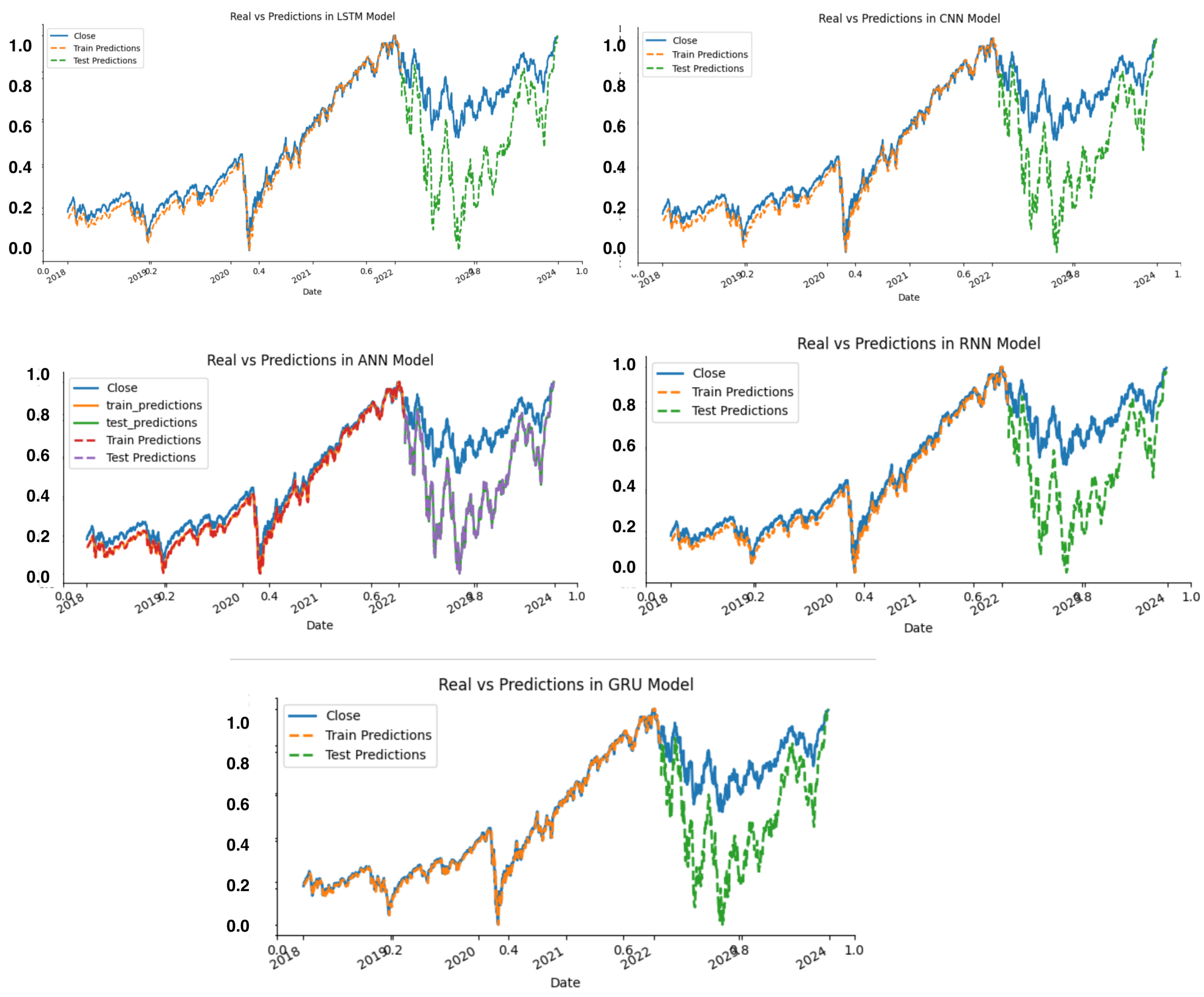
Evaluate the model using the test data to predict future values.
Sklearn metrics RMSE and MAPE; directional_accuracy
Visualization:
Scatterplot train predictions, and test prediction.

References

  1. Abadi, Martín, Ashish Agarwal, Paul Barham, Eugene Brevdo, Zhifeng Chen, Craig Citro, Greg S. Corrado, Andy Davis, Jeffrey Dean, Matthieu Devin, and et al. 2016. Tensorflow: Large-scale machine learning on heterogeneous distributed systems. arXiv arXiv:1603.04467. [Google Scholar]
  2. Abhyankar, Abhay, Laurence S. Copeland, and Woon Wong. 1997. Uncovering nonlinear structure in real-time stock-market indexes: The s&p 500, the dax, the nikkei 225, and the ftse-100. Journal of Business & Economic Statistics 15: 1–14. [Google Scholar]
  3. Aldhyani, Theyazn H. H., and Ali Alzahrani. 2022. Framework for predicting and modeling stock market prices based on deep learning algorithms. Electronics 11: 3149. [Google Scholar] [CrossRef]
  4. Atsalakis, George S., and Kimon P. Valavanis. 2009. Surveying stock market forecasting techniques—Part II: Soft computing methods. Expert Systems with Applications 36: 5932–41. [Google Scholar] [CrossRef]
  5. Ayyildiz, Nazif, and Omer Iskenderoglu. 2024. How effective is machine learning in stock market predictions? Heliyon 10: e24123. [Google Scholar] [CrossRef] [PubMed]
  6. Azoff, E. Michael. 1994. Neural Network Time Series Forecasting of Financial Markets. New York: John Wiley & Sons, Inc. [Google Scholar]
  7. Chen, Chunchun, Pu Zhang, Yuan Liu, and Jun Liu. 2020. Financial quantitative investment using convolutional neural network and deep learning technology. Neurocomputing 390: 384–90. [Google Scholar] [CrossRef]
  8. Chen, Tin-Chih Toly, Cheng-Li Liu, and Hong-Dar Lin. 2018. Advanced artificial neural networks. Algorithms 11: 102. [Google Scholar] [CrossRef]
  9. Chhajer, Parshv, Manan Shah, and Ameya Kshirsagar. 2022. The applications of artificial neural networks, support vector machines, and long–short term memory for stock market prediction. Decision Analytics Journal 2: 100015. [Google Scholar] [CrossRef]
  10. Cooper, Ilan, and Paulo Maio. 2019. Asset growth, profitability, and investment opportunities. Management Science 65: 3988–4010. [Google Scholar] [CrossRef]
  11. Cvilikas, Aurelijus. 2012. Bankinės rizikos valdymo ekonominio efektyvumo vertinimas mažmeninėje bankininkystėje. Doctoral dissertation, Kauno Technologijos Universitetas, Kaunas, Lithuania. [Google Scholar]
  12. Deng, Aqin. 2023. Database task processing optimization based on performance evaluation and machine learning algorithm. Soft Computing 27: 6811–21. [Google Scholar] [CrossRef]
  13. Encke, David. 2008. Neural network-based stock market return forecasting using data mining for variable reduction. In Data Warehousing and Mining: Concepts, Methodologies, Tools, and Applications. Pennsylvania: IGI Global, pp. 2476–93. [Google Scholar] [CrossRef]
  14. Erbas, Bahar Celikkol, and Spiro E. Stefanou. 2009. An application of neural networks in microeconomics: Input–output mapping in a power generation subsector of the us electricity industry. Expert Systems with Applications 36: 2317–26. [Google Scholar] [CrossRef]
  15. Eslamieh, Pegah, Mehdi Shajari, and Ahmad Nickabadi. 2023. User2vec: A novel representation for the information of the social networks for stock market prediction using convolutional and recurrent neural networks. Mathematics 11: 2950. [Google Scholar] [CrossRef]
  16. Fang, Zhen, Xu Ma, Huifeng Pan, Guangbing Yang, and Gonzalo R. Arce. 2023. Movement forecasting of financial time series based on adaptive lstm-bn network. Expert Systems with Applications 213: 119207. [Google Scholar] [CrossRef]
  17. Gao, Ya, Rong Wang, and Enmin Zhou. 2021. Stock prediction based on optimized lstm and gru models. Scientific Programming 2021: 4055281. [Google Scholar] [CrossRef]
  18. Hadavandi, Esmaeil, Hassan Shavandi, and Arash Ghanbari. 2010. Integration of genetic fuzzy systems and artificial neural networks for stock price forecasting. Knowledge-Based Systems 23: 800–808. [Google Scholar] [CrossRef]
  19. Hansun, Seng, and Julio Christian Young. 2021. Predicting lq45 financial sector indices using rnn-lstm. Journal of Big Data 8: 1–13. [Google Scholar] [CrossRef]
  20. Hæke, Christian, and Christian Helmenstein. 1996. Neural networks in the capital markets: An application to index forecasting. Computational Economics 9: 37–50. [Google Scholar] [CrossRef]
  21. Kim, Sungil, and Heeyoung Kim. 2016. A new metric of absolute percentage error for intermittent demand forecasts. International Journal of Forecasting 32: 669–79. [Google Scholar] [CrossRef]
  22. Kuan, Chung-Ming, and Halbert White. 1994. Artificial neural networks: An econometric perspective. Econometric Reviews 13: 1–91. [Google Scholar] [CrossRef]
  23. Kumar, Krishna, and Md Tanwir Uddin Haider. 2021. Enhanced prediction of intra-day stock market using metaheuristic optimization on rnn–lstm network. New Generation Computing 39: 231–72. [Google Scholar] [CrossRef]
  24. Leung, Mark T., Hazem Daouk, and An-Sing Chen. 2000. Forecasting stock indices: A comparison of classification and level estimation models. International Journal of Forecasting 16: 173–90. [Google Scholar] [CrossRef]
  25. Li, Haosong, and Phillip C.-Y. Sheu. 2022. A scalable association rule learning and recommendation algorithm for large-scale microarray datasets. Journal of Big Data 9: 35. [Google Scholar] [CrossRef]
  26. Li, Shaoyu, Kaixuan Ning, and Teng Zhang. 2021. Sentiment-aware jump forecasting. Knowledge-Based Systems 228: 107292. [Google Scholar] [CrossRef]
  27. Lin, Shih-Lin, and Hua-Wei Huang. 2020. Improving deep learning for forecasting accuracy in financial data. Discrete Dynamics in Nature and Society 2020: 5803407. [Google Scholar] [CrossRef]
  28. Lin, Tsong-Wuu, and Chan-Chien Yu. 2009. Forecasting stock market with neural networks. Computer Science Business Economics, 1–14. [Google Scholar] [CrossRef]
  29. Lu, Wenjie, Jiazheng Li, Jingyang Wang, and Lele Qin. 2021. A cnn-bilstm-am method for stock price prediction. Neural Computing and Applications 33: 4741–53. [Google Scholar] [CrossRef]
  30. Ma, Chenyao, and Sheng Yan. 2022. Deep learning in the chinese stock market: The role of technical indicators. Finance Research Letters 49: 103025. [Google Scholar] [CrossRef]
  31. Maris, Konstantinos, Konstantinos Nikolopoulos, Konstantinos Giannelos, and Vassilis Assimakopoulos. 2007. Options trading driven by volatility directional accuracy. Applied Economics 39: 253–60. [Google Scholar] [CrossRef]
  32. Markowitz, Harris. 1952. Portfolio Selection. The Journal of Finance 7: 77–91. [Google Scholar]
  33. Matkovskyy, Roman, and Taoufik Bouraoui. 2019. Application of neural networks to short time series composite indexes: Evidence from the nonlinear autoregressive with exogenous inputs (narx) model. Journal of Quantitative Economics 17: 433–46. [Google Scholar] [CrossRef]
  34. McKinney, Wes. 2010. Data structures for statistical computing in python. Paper presented at the 9th Python in Science Conference, Austin, TX, USA, 28 June–3 July 2010; vol. 445, pp. 51–56. [Google Scholar]
  35. Meese, Richard A., and Andrew K. Rose. 1991. An empirical assessment of non-linearities in models of exchange rate determination. The Review of Economic Studies 58: 603–19. [Google Scholar] [CrossRef]
  36. Moghaddam, Amin Hedayati, Moein Hedayati Moghaddam, and Morteza Esfandyari. 2016. Stock market index prediction using artificial neural network. Journal of Economics, Finance and Administrative Science 21: 89–93. [Google Scholar] [CrossRef]
  37. Moghar, Adil, and Mhamed Hamiche. 2020. Stock market prediction using lstm recurrent neural network. Procedia Computer Science 170: 1168–73. [Google Scholar] [CrossRef]
  38. Mostafa, Mohamed M., and Ahmed A. El-Masry. 2016. Oil price forecasting using gene expression programming and artificial neural networks. Economic Modelling 54: 40–53. [Google Scholar] [CrossRef]
  39. O’Doherty, Michael S. 2012. On the conditional risk and performance of financially distressed stocks. Management Science 58: 1502–20. [Google Scholar] [CrossRef]
  40. Puh, Karlo, and Marina Bagić Babac. 2023. Predicting stock market using natural language processing. American Journal of Business 38: 41–61. [Google Scholar] [CrossRef]
  41. Qi, Chenyang, Jiaying Ren, and Jin Su. 2023. Gru neural network based on ceemdan–wavelet for stock price prediction. Applied Sciences 13: 7104. [Google Scholar] [CrossRef]
  42. Qi, Min. 1996. 18 financial applications of artificial neural networks. Handbook of Statistics 14: 529–52. [Google Scholar]
  43. Raudys, Aistis, and Edvinas Goldstein. 2022. Forecasting detrended volatility risk and financial price series using lstm neural networks and xgboost regressor. Journal of Risk and Financial Management 15: 602. [Google Scholar] [CrossRef]
  44. Reboredo, Juan C., José M. Matías, and Raquel Garcia-Rubio. 2012. Nonlinearity in forecasting of high-frequency stock returns. Computational Economics 40: 245–64. [Google Scholar] [CrossRef]
  45. Rikukawa, Shota, Hiroki Mori, and Taku Harada. 2020. Recurrent neural network based stock price prediction using multiple stock brands. International Journal of Innovative Computing, Information and Control 16: 1093–99. [Google Scholar]
  46. Sako, Kady, Berthine Nyunga Mpinda, and Paulo Canas Rodrigues. 2022. Neural networks for financial time series forecasting. Entropy 24: 657. [Google Scholar] [CrossRef]
  47. Sandoval Serrano, Lilian Judith. 2018. Algoritmos de Aprendizaje Automático Para Análisis y Predicción de Datos. Revista Tecnológica; no. 11. El Salvador: ITCA. [Google Scholar]
  48. Sheth, Dhruhi, and Manan Shah. 2023. Predicting stock market using machine learning: Best and accurate way to know future stock prices. International Journal of System Assurance Engineering and Management 14: 1–18. [Google Scholar] [CrossRef]
  49. Song, Hyunsun, and Hyunjun Choi. 2023. Forecasting stock market indices using the recurrent neural network based hybrid models: Cnn-lstm, gru-cnn, and ensemble models. Applied Sciences 13: 4644. [Google Scholar] [CrossRef]
  50. Stasinakis, Charalampos, Georgios Sermpinis, Konstantinos Theofilatos, and Andreas Karathanasopoulos. 2016. Forecasting us unemployment with radial basis neural networks, kalman filters and support vector regressions. Computational Economics 47: 569–87. [Google Scholar] [CrossRef]
  51. Ticknor, Jonathan L. 2013. A bayesian regularized artificial neural network for stock market forecasting. Expert Systems with Applications 40: 5501–6. [Google Scholar] [CrossRef]
  52. Van Der Walt, Stefan, S. Chris Colbert, and Gael Varoquaux. 2011. The numpy array: A structure for efficient numerical computation. Computing in Science & Engineering 13: 22–30. [Google Scholar]
  53. Van Greuning, Hennie, and Sonja Brajovic Bratanovic. 2020. Analyzing Banking Risk: A Framework for Assessing Corporate Governance and Risk Management. Washington: World Bank Publications. [Google Scholar] [CrossRef]
  54. Villada, Fernando, Nicolás Muñoz, and Edwin García. 2012. Aplicación de las redes neuronales al pronóstico de precios en el mercado de valores. Información tecnológica 23: 11–20. [Google Scholar] [CrossRef]
  55. von Spreckelsen, Christian, Hans-Jörg von Mettenheim, and Michael H. Breitner. 2014. Real-time pricing and hedging of options on currency futures with artificial neural networks. Journal of Forecasting 33: 419–32. [Google Scholar] [CrossRef]
  56. Wang, Xingyuan, Lintao Liu, and Yingqian Zhang. 2015. A novel chaotic block image encryption algorithm based on dynamic random growth technique. Optics and Lasers in Engineering 66: 10–18. [Google Scholar] [CrossRef]
  57. Wang, Yimeng, and Keyue Yan. 2023. Machine learning-based quantitative trading strategies across different time intervals in the american market. Quantitative Finance and Economics 7: 569–94. [Google Scholar] [CrossRef]
  58. Zhang, Shuwen, and Wen Fang. 2021. Multifractal behaviors of stock indices and their ability to improve forecasting in a volatility clustering period. Entropy 23: 1018. [Google Scholar] [CrossRef] [PubMed]
  59. Zhang, Yaojie, Feng Ma, and Yu Wei. 2019. Out-of-sample prediction of the oil futures market volatility: A comparison of new and traditional combination approaches. Energy Economics 81: 1109–20. [Google Scholar] [CrossRef]
  60. Zhang, Yaojie, Likun Lei, and Yu Wei. 2020. Forecasting the chinese stock market volatility with international market volatilities: The role of regime switching. The North American Journal of Economics and Finance 52: 101145. [Google Scholar] [CrossRef]
  61. Zhang, Yongjie, Gang Chu, and Dehua Shen. 2021. The role of investor attention in predicting stock prices: The long short-term memory networks perspective. Finance Research Letters 38: 101484. [Google Scholar] [CrossRef]
  62. Zheng, Yuanhang, Zeshui Xu, and Anran Xiao. 2023. Deep learning in economics: A systematic and critical review. Artificial Intelligence Review 56: 9497–539. [Google Scholar] [CrossRef]
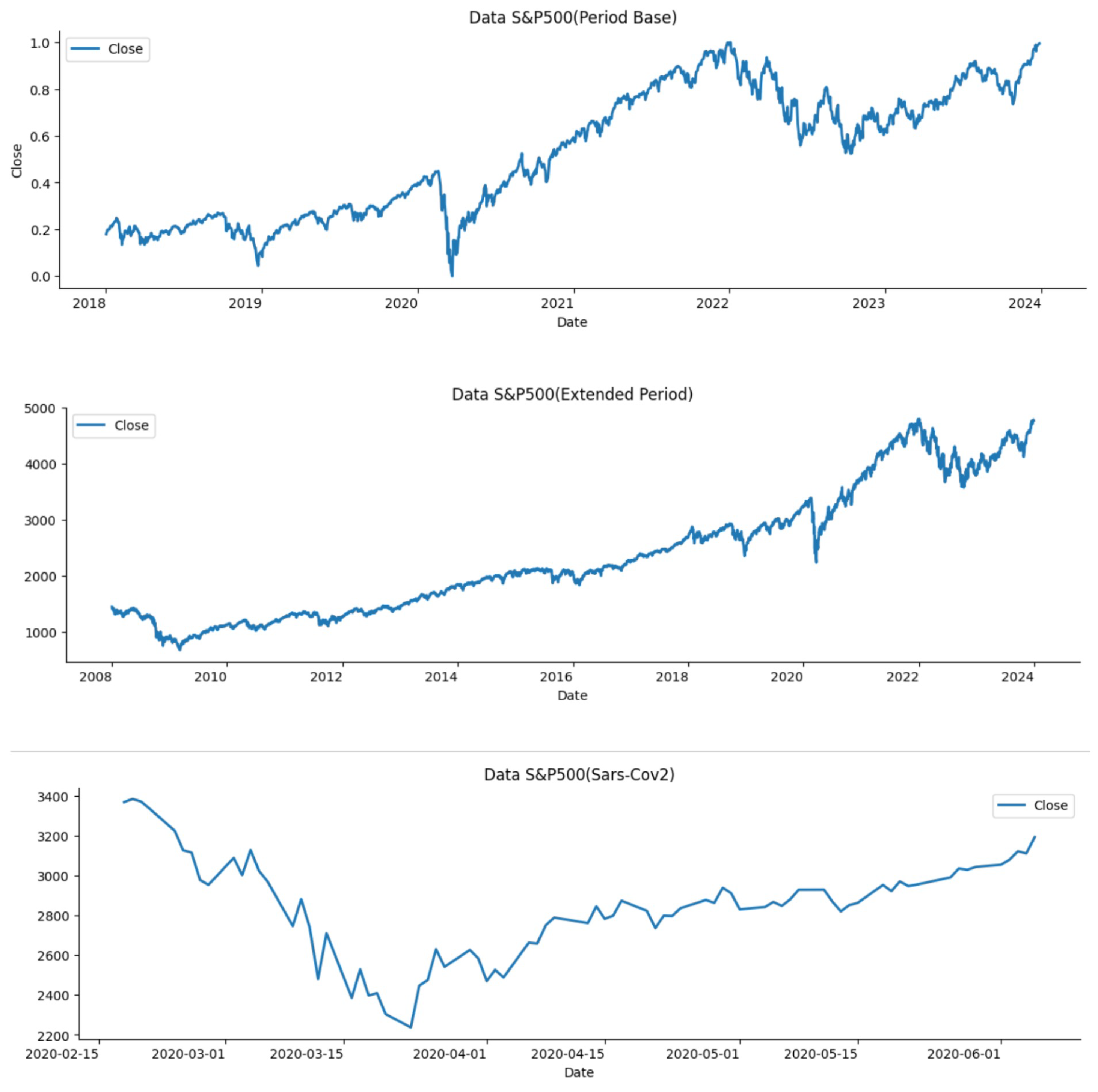
Figure 1. Data applied in neural network models.
Jrfm 17 00242 g001
Figure 2. Epoch rolling RMSE.
Jrfm 17 00242 g002
Figure 3. Adjusted model, train, test and real data.
Jrfm 17 00242 g003
Table 1. S&P500 data.
Close (Period Base)Close Extended PeriodClose SARS-CoV-2
count1508.0000004023.00000074.000000
mean3587.1127382353.1592940.530256
std691.0919281112.9265750.218452
min2237.399902676.5300290.000000
25%2888.2925421354.5349730.434525
50%3676.3950202087.7900390.545201
75%4204.1599123004.2800290.656688
max4796.5600594796.5600591.000000
Table 2. Indices applied by previous authors.
Data UsedAuthors
DJIAPuh and Bagić Babac (2023)
Apple Inc. (AAPL)
IBM Corporation (IBM)
Microsoft (MSFT)
Goldman Sachs (GS)
    Ticknor (2013)
S&P500Abhyankar et al. (1997); Lin and Yu (2009); Zhang et al. (2021)
NasdaqMoghaddam et al. (2016)
Shanghai Composite IndexLu et al. (2021)
CAX40, DAX and the Greek
FTSE/ASE 20 stock
Abhyankar et al. (1997); Maris et al. (2007)
Tokyo Stock ExchangeRikukawa et al. (2020)
Nikkei 225Abhyankar et al. (1997); Moghar and Hamiche (2020)
GOOGL, NKEMoghar and Hamiche (2020)
Chinese stock MarketMa and Yan (2022)
SSE 50 indexZhang et al. (2021)
MSCI Emerging Markets IndexZhang et al. (2020)
Table 3. Parameters of neural network models.
FeatureANNCNNLSTMRNNGRU
Layer StructureSequentialSequentialSequentialSequentialSequential
Hidden LayersANN with 50 unitsCNNLSTM with 50 unitsSimpleRNN with 50 unitsGRU with 50 units
Convolutional
Layers
NoneConv1D with 64 filters, kernel size 2, ReLU activationNoneNoneNone
Pooling LayerNoneMaxPooling1D, pool size 2NoneNoneNone
Flatten LayerNoneFlattenNoneNoneNone
Output LayerDense with 1 unitDense with 1 unitDense with 1 unitDense with 1 unitDense with 1 unit
Data NormalizationMinMax
Scaler
MinMax
Scaler
MinMax
Scaler
MinMax
Scaler
MinMax Scaler
Callback 2EarlyStoppingEarlyStoppingEarlyStoppingEarlyStoppingEarlyStopping
Data PreparationSliding windowsSliding windowsSliding windowsSliding windowsSliding windows
Time Window33333
Number of Epochs500500500500500
Optimal Epoch
(Date Model Base)
50010628528500
Optimal Epoch
(Extended period)
21373128500
Optimal Epoch
(SARS-CoV-2)
137265134100500
Table 4. Error metrics of neural network models: RMSE and MAPE.
RMSEMAPERMSE
Long Period
MAPE
Long Period
RMSE
SARS-CoV-2
MAPE
SARS-CoV-2
LSTM0.02508932.7557%0.03203.1168%0.069769.4737%
CNN0.02556812.7954%0.01461.3137%0.042625.3049%
ANN0.03034224.6388%0.01481.1291%0.038215.1252%
RNN0.03644915.6406%0.014691.3327%0.058037.8447%
GRU0.02033392.2018%0.01661.4994%0.0446510.6185%
Table 5. Directional accuracy.
Directional Accuracy TrainDirectional Accuracy TestDirectional Accuracy Train Long PeriodDirectional Accuracy Test Long PeriodDirectional Accuracy Train SARS-CoV-2Directional Accuracy Test SARS-CoV-2
LSTM50.50%49.30%47.29%50.50%47.70%49.30%
CNN48.70%56.91%49.50%46.69%48.30%52.71%
ANN47.90%48.10%48.70%52.10%44.89%51.70%
RNN47.09%49.90%48.50%51.70%50.10%45.29%
GRU51.10%49.90%50.70%48.30%49.30%49.90%
Disclaimer/Publisher’s Note: The statements, opinions and data contained in all publications are solely those of the individual author(s) and contributor(s) and not of MDPI and/or the editor(s). MDPI and/or the editor(s) disclaim responsibility for any injury to people or property resulting from any ideas, methods, instructions or products referred to in the content.

