Abstract
This study confirms gold’s role as a reliable inflation hedge while introducing new insights into lesser-explored assets like art and wheat. Using advanced methodologies such as the ARDL framework and LSTM deep learning, it conducts a detailed analysis of inflation-hedging dynamics, exploring non-linear relationships and unexpected inflation impacts across various asset classes. The findings reveal complex dynamics. Gold demonstrates strong long-term inflation hedging potential. The negative coefficient for the US dollar index suggests that gold acts as a hedge against currency depreciation. Furthermore, a positive relationship between gold returns and inflation during high inflation periods highlights its effectiveness in protecting purchasing power. Art presents a more intricate picture. Long-term analysis suggests a weak mean-reverting tendency, but a negative relationship with inflation, potentially linked to economic downturns. Interestingly, unexpected inflation positively correlates with art returns in the long run, hinting at its potential inflation-hedging abilities. No statistically significant connection between wheat prices and overall inflation was observed; the short-run analysis reveals a dynamic interplay between inflation, real GDP growth, and wheat prices at different time points.
1. Introduction
Inflation hedging is a perennial focal point for investors navigating the chaotic waters of financial markets. The relentless march of rising prices challenges wealth preservation, prompting a genuine quest for assets capable of safeguarding against the erosive effects of inflation (Attié and Roache 2009). Over the years, many studies spanning diverse asset classes and market conditions have scrutinized the efficacy of various instruments as inflation hedges, illuminating the intricate interplay between economic forces and investment strategies.
Renowned for its historical precedence and limited supply, gold is uniquely positioned in the pantheon of inflation hedges. While proponents extol its long-term correlation with inflation, underscored by studies from Chiang (2023), McCown and Zimmerman (2010), and Xu et al. (2021), skeptics caution against overestimating its reliability, as evidenced by research from Brown et al. (2023) and Ghazali et al. (2015).
Venturing beyond precious metals, real estate, housing, and REITs are also potential bulwarks against inflationary pressures. The landscape of real estate investment is fraught with complexities, as highlighted by studies from Chiang (2023), Lee (2014), and Nguyen (2023). While some tout real estate’s long-term hedging potential, others caution against short-term fluctuations and market heterogeneity, underscoring the need for a granular understanding of geographic, sectoral, and temporal dynamics. Within this milieu, REITs emerge as a hybrid entity, offering indirect exposure to real estate while navigating the intricacies of lease contracts and management fees. However, their inflation-hedging efficacy remains debatable, as Gyourko and Linneman (1988) and de Wit (2023) elucidated.
The advent of cryptocurrencies heralds a paradigm shift in inflation hedging, injecting a dose of digital disruption into traditional investment paradigms. While some herald Bitcoin as a panacea for inflation hedging, others caution against its volatility and limited empirical evidence, as expounded by Choi and Shin (2022), Arshad et al. (2023), and Smales (2024).
Turning the attention towards traditional bastions of investment, the realm of stocks and bonds as potential bulwarks against inflation cannot be ignored. The Fisher hypothesis lays bare the theoretical underpinnings of stock performance in the face of inflation, yet empirical evidence reveals a more nuanced reality, as elucidated by Ciner (2015). Likewise, bonds confront a dichotomy between nominal bonds’ vulnerability to inflation and the allure of inflation-protected bonds, as articulated by Eagle and Domian (1995) and Papathanasiou et al. (2023).
This study seeks to address a notable gap in the inflation hedge literature by examining the inflation-hedging potential of two often overlooked asset classes: wheat and art. While gold has garnered substantial attention in inflation hedge research, wheat and art have remained relatively underexplored despite their potential significance in diversifying inflation-hedging strategies. By incorporating wheat and art into the broader landscape of inflation hedge research, this study aims to provide a more comprehensive understanding of inflation-hedging strategies. By elucidating the potential role of these asset classes in preserving purchasing power and mitigating inflationary risks, this study seeks to empower investors with a more diversified toolkit for navigating the complexities of inflationary environments. Through rigorous empirical analysis and academic inquiry, this study contributes to the growing body of knowledge on inflation hedging, fostering a deeper understanding of the intersection between financial markets and real-world economic dynamics.
In the present study, the ARDL framework is employed to investigate the inflation-hedging potential of gold, art, and wheat using US data from 1992 to 2023. This approach offers an advantage over traditional linear models by considering potential nonlinearities in the relationship between inflation and the returns of these assets. This allows for a more comprehensive understanding of how asset prices react to positive and negative inflation shocks in the short run.
The empirical findings reveal dynamics regarding the inflation-hedging abilities of gold, art, and wheat. Gold emerges as a significant inflation hedge, particularly over the long term, with its negative coefficient for past prices indicating a mean-reverting tendency and its negative coefficient for the US dollar index supporting its role as a hedge against currency depreciation. Moreover, a positive relationship between gold returns and CPI during high inflation regimes underscores its function as a safeguard against purchasing power erosion. Art’s inflation hedge potential presents a more complex picture, with long-term analyses suggesting a weak mean-reverting tendency but a negative relationship between inflation and art returns, potentially attributed to economic downturns. However, unexpected inflation positively correlates with art returns in the long run, indicating its potential as an inflation hedge. Wheat also demonstrates mean-reverting tendencies in the long run, with a negative coefficient for the US dollar index suggesting a potential negative association with a stronger dollar. Although no statistically significant relationship between wheat prices and inflation is found, the short-run analysis reveals a dynamic interplay between inflation, real GDP growth, and wheat prices at different time points.
This study investigates gold, art, and wheat inflation-hedging abilities in the United States from 1992 to 2023. Research questions include examining whether gold, art, and wheat are effective hedges against inflation and currency depreciation over different time horizons. Hypotheses propose that gold will demonstrate mean-reverting behavior and a positive correlation with the Consumer Price Index (CPI) during periods of high inflation. Conversely, art may exhibit sensitivity to economic downturns, but could potentially serve as a hedge against unexpected inflation. Wheat is hypothesized to show mean-reverting tendencies and interact with economic growth indicators, although its relationship with inflation may vary across short- and long-term analyses. These investigations provide critical insights for investors and policymakers aiming to manage inflation risks and optimize asset allocation strategies in diverse economic environments.
2. Literature Review on Inflation Hedging
Inflation hedging has long been a topic of interest for investors seeking to protect their portfolios from the erosive effects of rising prices. Many studies spanning various asset classes and market conditions have examined the efficacy of different instruments as inflation hedges. This study explores the various asset classes discussed in the inflation hedge literature. It categorizes these assets into five main groups: (1) the classic inflation hedge, gold, is examined for its historical performance and limited supply; (2) the study explores real estate options like housing and REITs, which tend to maintain value and potentially appreciate with inflation; (3) it examines a more recent area of investigation, with some suggesting crypto’s potential for protection, but its volatility raises questions about its reliability; (4) the study then analyzes the broad category of stocks and bonds. While traditional bonds generally lose purchasing power with inflation, stocks can outperform them in the long run. However, the focus shifts to inflation-linked bonds, specifically designed to adjust for inflation; and (5) the study acknowledges the existence of other potential hedges such as commodities, wheat, infrastructure investments, and even collectibles, highlighting the need for further exploration of their effectiveness under varying economic conditions.
2.1. Gold as an Inflation Hedge
Several studies provide compelling evidence that gold can be an effective inflation hedge. Proponents of gold as a hedge highlight the long-run correlation between gold prices and inflation. Research by Chiang (2023), McCown and Zimmerman (2010), and Xu et al. (2021) has suggested a positive correlation over extended periods. This implies that gold prices rise alongside inflation, helping investors maintain purchasing power in the long run. This long-term positive correlation offers stability and predictability for investors seeking protection against the erosion of their assets’ value due to inflation.
Furthermore, studies by Conlon et al. (2018) and Afham et al. (2017) have suggested that gold can effectively hedge short-term and long-term inflation. This versatility offers investors flexibility in tailoring their inflation protection strategies. The “safe haven” role of gold during periods of high inflation or economic uncertainty is another factor supporting its effectiveness as a hedge. Research by Iqbal (2017) strengthened this argument. When traditional asset classes experience significant devaluation due to economic turmoil, investors may flock to gold, increasing its price. This flight-to-safety behavior during periods of crisis underscores gold’s potential to provide a degree of protection for investors’ wealth.
Despite the arguments presented above, other studies raise concerns about the reliability of gold as an inflation hedge. Notably, research by Brown et al. (2023) and Ghazali et al. (2015) found a weak or insignificant relationship between gold prices and inflation in some instances. This suggests that gold may only sometimes provide a consistent and reliable hedge against inflation. Investors relying solely on gold during such periods might experience unexpected erosion of purchasing power if gold prices keep up with inflation. The effectiveness of gold as a hedge can vary depending on the specific country or economic situation, as highlighted by Van Hoang et al. (2016) and Wang et al. (2011). Local monetary policy and economic structure can influence the relationship between gold prices and inflation in different regions. This variability necessitates an approach whereby investors consider the global dynamics of gold prices and inflation and the specific economic context of their own country. Thi Thanh Binh (2023) further supported this point by examining the case of Vietnam, where gold and the US dollar strongly responded to inflation, highlighting the need for country-specific analysis.
Even when gold prices increase alongside inflation, the increase might not fully compensate for the inflation rate, leaving investors with some degree of purchasing power erosion. Research by Shahbaz et al. (2014) and Wang et al. (2013) has supported this notion. This “incomplete hedging” effect highlights the limitations of gold as a perfect inflation hedge. Investors should be aware of this potential gap and consider it when evaluating their inflation protection strategies.
2.2. Real Estate, Housing, and REITs as Inflation Hedges
Real estate, housing, and Real Estate Investment Trusts (REITs) have long been touted as potential hedges against inflation, but the reality is far from a simple yes or no answer. Unraveling the intricacies of real estate, housing, and REITs as inflation hedges reveals a dynamic interplay between asset type, temporal considerations, and market characteristics. While studies by Chiang (2023) and Lee (2014) have suggested a positive correlation between inflation and asset prices, offering a potential shield, the effectiveness varies. The time horizon emerges as a critical factor. Research by Lee (2014) and Amenc et al. (2009) indicated real estate’s strength as a long-term hedge, with cointegration analysis suggesting prices eventually adjust to inflation. However, Taderera and Akinsomi (2020) highlighted potential short-term fluctuations, with commercial real estate exhibiting hedging properties only in the short run.
Heterogeneity across markets plays a significant role. Dittmann (2024) and Essafi Zouari and Nasreddine (2024) emphasized how location, property type, and investment horizon influence hedging effectiveness. Residential properties in booming areas might outperform those in stagnant markets. Similarly, commercial properties catering to specific industries may react differently to inflation than residential housing. Additionally, Dittmann (2024) suggested that longer investment horizons benefit more from real estate’s inflation-hedging properties. Recent work by Nguyen (2023) employing deep learning techniques found that housing returns in Japan and the USA were able to hedge against inflation between 2000 and 2020, supporting Fisher’s hypothesis. Previously, studies by Nguyen and Wang (2010) and Fang et al. (2008) explicitly examining the Taiwanese housing market from 1991 to 2006 found a negative relationship between housing returns and both expected and unexpected inflation. This suggests that housing in Taiwan during that period did not effectively hedge against inflation. The authors attributed this to leverage shocks and opportunistic investor behavior. Kuan-Min et al. (2008) further highlighted the importance of considering inflation regimes, as their research suggested a threshold effect, with housing returns only hedging against inflation exceeding a specific level.
The equation gets even more intricate with REITs. Offering indirect exposure, their behavior deviates from direct ownership. Gyourko and Linneman (1988) found REIT returns to be less correlated with inflation. Lease contracts and management fees can decouple REIT returns from underlying property value appreciation, potentially weakening their inflation-hedging abilities. However, de Wit (2023) introduced an interesting wrinkle: real estate might be a better hedge against unexpected inflation. Lease agreements with inflation adjustments can further enhance this protection.
2.3. Cryptocurrencies and Bitcoin as Inflation Hedges
The allure of cryptocurrencies as shields against inflation has sparked a lively debate within the financial world. While some studies offer promising results, a clear consensus still needs to be discovered. Choi and Shin (2022) presented evidence suggesting Bitcoin appreciates alongside inflation, potentially acting as a hedge. Arshad et al. (2023) bolstered this notion by indicating that Bitcoin might function as a hedge and safe haven in Southeast Asian countries. However, Smales (2024) tempered this optimism, finding a positive association between Bitcoin returns and inflation expectations only under specific circumstances, particularly when inflation remains low. This limited hedging power was further highlighted by Phochanachan et al. (2022), who found that Bitcoin’s effectiveness wanes in the long run. The picture becomes even more intricate when considering the evolving dynamics. Sakurai and Kurosaki (2023) suggested that major cryptocurrencies might have become slightly better hedges following the economic reopening after COVID-19. Liu and Valcarcel (2024) added another layer by exploring Bitcoin futures. Their research found a positive correlation between Bitcoin futures prices and inflation expectations, suggesting these instruments offer a hedge against anticipated inflation, but with diminished effectiveness during periods of heightened market uncertainty.
2.4. Stocks and Bonds as Inflation Hedges
This comprehensive review examined the effectiveness of stocks and bonds as inflation hedges. While the Fisher hypothesis suggests stocks should keep pace with inflation, the reality is more nuanced. Studies supporting stocks as long-term hedges must be evaluated for potential biases like survivorship bias. The effectiveness might also vary by stock type (Ciner 2015), highlighting the importance of sector selection. Additionally, positive correlation with unexpected inflation (Ciner 2015) warrants further investigation using robust methodologies. Nominal bonds, as expected (Eagle and Domian 1995), are poor inflation hedges due to their fixed payouts. Inflation-protected bonds (TIPS) address this issue (Papathanasiou et al. 2023), but their liquidity compared to nominal bonds requires further exploration.
Some studies (Alagidede and Panagiotidis 2010; Bampinas and Panagiotidis 2016) have found that stocks, particularly those in cyclical sectors like energy and industrials, exhibit a positive long-run relationship with inflation. This suggests that stock prices tend to rise with inflation, potentially offering some protection against its erosive effects. However, another study (Spierdijk and Umar 2015) found limited evidence for this relationship, particularly in the short run. They argued that other factors, such as economic growth and interest rates, can significantly influence stock prices, making their inflation-hedging capabilities unreliable.
Long-term bonds are generally considered poor inflation hedges (Spierdijk and Umar 2015; Brown et al. 2023). As inflation rises, the fixed interest rate payments on bonds become less valuable in real terms. Additionally, the price of long-term bonds can fall significantly when interest rates rise to combat inflation. However, some studies have suggested that short-term bonds or specific bond strategies can offer some inflation protection. Bruno and Chincarini (2011) find that short-term bonds can be incorporated into a multi-asset portfolio to enhance its inflation-hedging capabilities.
2.5. Other Assets as an Inflation Hedge
Several studies have delved into commodities as a potential hedge. Bird (1984) explored commodities traded on the London market, highlighting tin as a suitable individual hedge. Zaremba et al. (2019) utilized extensive historical data to demonstrate the inflation-hedging properties of commodities across various timeframes and geographies, emphasizing the importance of diversification within commodities. However, Brown et al. (2023) presented a contrasting view, suggesting that a diversified basket of commodities and wheat may be more effective than traditional choices.
Cheng et al. (2023) introduced a novel framework that personalizes inflation-hedging strategies based on individual circumstances. They argued that traditional portfolio optimization may not adequately address short-term inflation concerns, and proposed incorporating an investor’s personalized inflation rate into asset allocation decisions. Salisu et al. (2020) highlighted the dynamic nature of inflation hedging for commodities like coal, iron ore, and cocoa, where effectiveness hinges on factors like net export status and investment horizon. These findings caution against static models and advocate for flexible strategies that adapt to changing market conditions.
Zhang et al. (2024) found that art serves as a long-term inflation hedge in France due to its robust market and supportive policies, contrasting with its negligible hedging impact in the US and UK. Öztürkkal and Togan-Eğrican (2020) showed that Turkish art exhibits a low correlation with equities, suggesting it diversifies investment portfolios.
Furthermore, the research has exposed the heterogeneity within asset classes themselves. Brown et al. (2023) challenged the conventional wisdom of gold and TIPS as reliable hedges, proposing a diversified basket of commodities and wheat as a potentially superior option. Baral and Mei (2023) added another layer of complexity by demonstrating that private-equity farmland offers protection against all inflation types, while timberland is effective against expected and unexpected inflation. Ciner (2015) even suggested that equities in specific sectors, like commodities and technology, may hedge against unexpected inflation. This heterogeneity underscores the importance of asset selection that aligns with an investor’s specific inflation hedging goals.
Figure 1 provides a roadmap for understanding how different asset classes can be used as inflation hedges. The most recent data points are highlighted in yellow, allowing for easy identification of trends. Lines connecting various asset classes potentially represent research that has analyzed their effectiveness in combating inflation. The figure itself categorizes assets into two main groups: “Real Assets” and “Financial Assets”. This research enhances the literature by providing detailed insights into how gold, art, and wheat serve as inflation hedges, addressing a specific gap in current knowledge. It not only advances theoretical understanding but also offers practical guidance for stakeholders in investment and policy contexts. The use of advanced methods such as the ARDL framework and LSTM deep learning adds methodological rigor, enabling a nuanced analysis of non-linear relationships and unexpected inflation impacts.
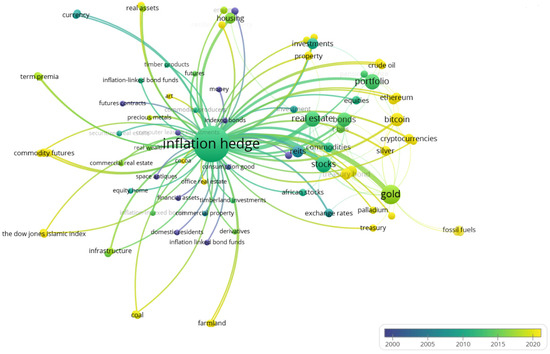
Figure 1.
Map of the inflation hedge literature.
3. Research Methodology
3.1. Linear vs. Nonlinear ARDL
The autoregressive distributed lag (ARDL) model, pioneered by Pesaran and Shin (1995) and Pesaran et al. (2001), is a specific linear time series model type. These models capture the relationship between dependent and independent variables, considering both contemporaneous effects (current values) and lagged effects (influence from past values). In other words, ARDL is a regression model estimated using ordinary least squares (OLS) that incorporate past values (lags) of both the dependent variable and the explanatory variables as regressors (Greene 2008).
where denotes the dependent variable at time t, represents the coefficient on the jth lag of the dependent variable, signifies the value of the explanatory variable at time t-j (jth lag), represents the coefficient on the jth lag of the rth explanatory variable, denotes the sth exogenous variable at time t, signifies the coefficient of the sth exogenous variable, and represents the error term at time t.
The linear ARDL framework posits a long-run equilibrium relationship that is a linear combination of the regressors. While this assumption serves as a convenient starting point, it may not fully capture the complexities observed in real-world phenomena. The fields of finance and economics highlight the prevalence of nonlinearities and asymmetries in economic behavior. Shin et al. (2014) introduced the nonlinear ARDL (NARDL) framework to address this limitation. This novel approach incorporated short- and long-run nonlinearities by decomposing the explanatory variables into positive and negative partial sum components.
The variable is decomposed into its partial sums relative to a threshold value . This decomposition is represented as . The variable is expressed as the sum of two separate processes, and . These processes capture the positive and negative deviations of from the threshold , respectively.
The intertemporal dynamics (ITD) representation of a model is given by:
This notation utilizes the vector to represent coefficients associated with the initial conditions of the model. Additionally, and are distinct coefficients specific to the asymmetric distributed-lag variables, which suggests a differential impact of past values on the present outcome.
where are asymmetric analogues of the coefficients. Through algebraic manipulation, it is possible to restructure Equation (4). This manipulation will result in a new equation that expresses the same relationship between variables but may be presented in a form more suitable for further analysis or interpretation.
To further refine the analysis, it is necessary to explicitly define the concept of an asymmetric equilibrium error correction term. This term captures the dynamic process by which variables adjust back towards a long-run equilibrium relationship. However, crucially, it allows for the speed of adjustment to differ depending on whether the deviation is positive or negative.
This transformation aims to express the conditional error correction (CEC) Equation (5) in the error correction (EC) form. By doing so, it can leverage the advantages of the EC framework for analysis, interpretation, and, potentially, further manipulation of the equation.
In Equation (7), the long-term equilibrium values for the explanatory variables are determined by the error correction parameter, denoted by . Specifically, these equilibrium values are obtained by and by φ, for r ranging from 1 to k (number of explanatory variables). In contrast, the short-term dynamics of the explanatory variables are captured by a different set of parameters: , , , and .
The CEC representation of ARDL and NARDL offers an advantage over their ITD representation by decomposing the influence of distribution lag variables. This decomposition separates the effects into short-run and long-run components. Consequently, the CEC representation allows for asymmetries in how these dynamics interact at different time scales. This flexibility in capturing these asymmetrical relationships is absent in the ITD representation, which treats the distribution lag effects as a single entity.
3.2. The Data Analysis
This study leverages the US dataset spanning over 31 years, from January 1992 to December 2023, with monthly observations. To assess the effectiveness of various assets as inflation hedges, this study incorporates price indexes for gold (sourced from the World Gold Council), art (using Art Market Research’s innovative valuation approach), and wheat (obtained from Macrotrends Data). Additionally, it analyzes key economic indicators, including the Consumer Price Index (CPI) from the International Monetary Fund (IMF) to gauge inflation, Real Gross Domestic Product (GDP) data from S&P Global to understand inflation-adjusted economic growth, and the US dollar index (sourced from Macrotrends Data) to track the value of the US dollar relative to other major currencies. This comprehensive dataset, encompassing asset prices and relevant economic factors at a monthly frequency, allows for a rigorous examination of how different asset classes perform against inflation over an extended period.
Figure 2 showcases historical data on various asset prices and economic indicators from 1992 to 2023, with all values presented on a logarithmic scale reflecting percentage changes. Asset prices, like gold (LGOLD) and art (LART), exhibit a generally upward trend with significant increases around 2008 and 2020, suggesting potential correlations with economic events. Wheat prices (LWHEAT) display more volatility, with spikes around 2008 and 2010 likely due to supply chain disruptions or other factors. Economic indicators paint a different picture. The consumer price index (LCPI), representing inflation, shows a gradual increase with steeper rises around 2008 and 2021. Real GDP (LRGDP) reflects economic growth with a positive trend, but experiences slower periods like the 2008 recession.
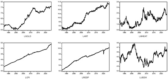
Figure 2.
The trends in asset prices and economic indicators.
The USD index (LUSDIX) indicates a slight downward trend over time, suggesting a weakening US dollar relative to other currencies. Interestingly, gold and art prices seem to rise alongside periods of inflation, potentially acting as hedges against rising costs. Economic growth also appears loosely correlated with some asset prices, suggesting increased demand during expansionary periods.
In line with Nguyen (2023), the long short-term memory (LSTM) model estimates both the expected and unexpected CPI. Hochreiter and Schmidhuber (1997) defined LSTM as an artificial recurrent neural network (RNN) architecture uniquely adept at addressing the vanishing gradient problem encountered in training data with varying gap lengths. Unlike traditional RNNs, LSTM networks exhibit relative insensitivity to gap length, making them well-suited for processing time series data with irregular intervals between significant events. The model, applied to monthly CPI data from January 1979 to December 2023, generates expected and unexpected inflation indices estimations. In Figure 3, the original CPI trend is depicted by the blue line, the expected CPI by the orange line, and the unexpected CPI by the green line. Notably, the model achieves an impressive predictive accuracy of 98.99%, indicating its efficacy in capturing the underlying patterns within the CPI data.
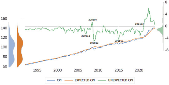
Figure 3.
Trends of CPI, expected CPI, and unexpected CPI in the United States from 1992 to 2023.
Figure 3 shows the CPI trend in the United States from 1992 to 2023. The graph illustrates three distinct periods: from 1992 to 2008, the CPI generally rose, notably spiking by over 30% between 2000 and 2008. Subsequently, from 2008 to 2015, the CPI remained relatively stable, experiencing minor fluctuations. However, from 2015 to 2020, there was a renewed upward trajectory, resulting in an overall 10% increase.
There has been a consistent upward trend in the CPI over the past quarter-century, with the most significant surge observed between 2000 and 2008, followed by a period of relative stability post-2008 and a subsequent rise from 2015 onwards. Expected CPI represents forecasted values, while unexpected CPI denotes disparities between actual and anticipated CPI. These positive or negative disparities serve as indicators of economic surprises, with large unexpected CPI figures suggesting unforeseen economic shifts.
The unexpected CPI can be used to measure economic surprises. A large unexpected CPI can indicate that something is happening in the economy that was not expected. As observed in Figure 2, the unexpected CPI data are highly volatile, particularly during periods of economic uncertainty. Fluctuations in unexpected CPI reflect the intricate interplay of various economic factors and policy decisions, underscoring the challenges of accurately forecasting inflationary trends. In December 2006, amidst the peak of the housing bubble in the United States, a negative unexpected CPI could have occurred due to artificially low housing prices.
Conversely, in July 2008, the onset of the recession could have led to a positive unexpected CPI, driven by a decline in economic activity and a surge in foreclosures. By December 2008, as the recession deepened, another negative unexpected CPI might have emerged, reflecting suppressed demand and prices. January 2015 marked a period of recovery from the recession, likely resulting in a slightly positive unexpected CPI as the economy experienced modest inflation. From February 2021 onwards, amid the COVID-19 pandemic, the unexpected CPI could have fluctuated. Initially, negative unexpected CPI might have occurred due to supply chain disruptions. However, as economies reopened, a shift to positive unexpected CPI could have ensued, driven by factors like pent-up demand and government stimulus programs.
Table 1 summarizes asset prices and economic indicators using descriptive statistics.

Table 1.
Descriptive statistics.
The average values (means) for gold (LGOLD) and art (LART) are significantly higher compared to wheat, suggesting they might represent prices on a larger scale. Looking at the spread of the data, the standard deviations (std. dev.) for all variables are relatively low, indicating the data clusters closely around their respective averages. Wheat prices (LWHEAT) and the USD index (LUSDIX) show the slightest variation, while wheat and real GDP (LRGDP) have slightly denser distributions around their centers. Interestingly, all skewness values are close to zero, implying a symmetrical distribution for most variables. This suggests that the data are not heavily skewed towards extreme values on either end.
Table 2 presents the results of unit root tests on variables at the level and after taking the first difference. The augmented Dickey–Fuller (ADF) test statistic is reported for each variable, along with the lag length used in the test. At the level, the ADF test statistics for LART, LGOLD, LWHEAT, LCPI, and LUSDIX suggest that these series may contain unit roots. After taking the first difference, all variables exhibit significant ADF test statistics at the 1% significance level, ranging from −6.385 to −20.878. This suggests that the first differences of all variables are stationary, supporting the use of integrated variables in subsequent analyses.
Table 2.
Unit root test.
The CEC representation of the ARDL and NARDL model investigating inflation involves utilizing the first difference of the logarithm of CPI and presents several notable benefits. CPI data often displays non-stationary behavior, wherein its statistical characteristics fluctuate over time, posing challenges for conventional time series analyses. Stationarity can be attained by applying a logarithmic transformation to CPI, thereby rendering the data more amenable to ARDL modeling. Additionally, the first difference of the logarithm of CPI captures the percentage change in inflation, offering a more interpretable metric than the raw CPI change. This facilitates a more transparent comprehension of how inflation fluctuations, whether positive or negative, affect the dependent variable within the model.
3.3. The Empirical Model
The linear ARDL model is applied to analyze the inflation-hedging ability of assets (gold, art, and wheat). The ARDL goes beyond traditional linear models by incorporating potential nonlinearities in the relationship between inflation (ΔLCPI) and asset prices. ΔLCPI captures the percentage change in inflation between two time periods. It is a more interpretable measure than the raw change in CPI because it expresses inflation as a percentage, making it easier to understand the impact of inflation fluctuations. Similarly, the first difference in the log of asset prices provides a clear picture of how asset returns vary over a given period, with positive values indicating gains and negative values indicating losses.
This allows for a better understanding of how asset prices respond to positive and negative inflation shocks in the short run. The CEC representation of the ARDL is as follows:
where is price of gold, art, and wheat, respectively.
The nonlinear ARDL (NARDL) can assess whether an asset and inflation are cointegrated in the long run, indicating the asset’s potential to hedge against inflation over time. is composed by , and the CEC empirical models with asymmetry inflation are defined as below:
represents the inflation regime, indicating periods where inflation is present, while represents the deflation regime, indicating periods where deflation occurs. The LCPI is undergoing a decomposition into four distinct variables to elucidate its underlying dynamics. This decomposition partitions the LCPI into positive and negative cumulative sums and cumulative difference sums, distinguishing between their long-term and short-term effects. Specifically, denoted by and are the positive and negative cumulative sums representing long-term effects, respectively. Meanwhile, and signify the positive and negative cumulative sums for short-term effects. Such a delineation facilitates a comprehensive examination of the factors influencing the LCPI over different time horizons, thereby enhancing the understanding of its behavior within economic contexts.
4. Empirical Results
The asymmetry tests analyze the influence of inflation on the prices of gold, art, and wheat. The test is crucial for understanding the relationship between inflation and asset prices. If the tests reveal a symmetrical relationship, meaning inflation and deflation have similar impacts, the linear ARDL model might suffice. However, if the relationship is asymmetrical, with inflation having a more substantial influence than deflation on asset prices, the study will employ the nonlinear ARDL to capture this asymmetry. The asymmetry test ensures that the chosen model accurately reflects the complex dynamics between inflation and the performance of these assets as inflation hedges.
Table 3 summarizes the results of coefficient symmetry tests examining the impact of LCPI on three dependent variables: LGOLD, LART, and LWHEAT. These tests aim to determine if the influence of LCPI differs across long-run and short-run timeframes.
Table 3.
Asymmetry tests for the influence of LCPI on assets.
The results reveal contrasting patterns. The statistically significant asymmetry of LGOLD is evident in the long run, suggesting the effect of LCPI on LGOLD is not constant over periods. Conversely, the short-run impact appears symmetrical, and the joint test hints at a potential overall asymmetry. In contrast to LGOLD, the results for LART strongly suggest a symmetrical influence of LCPI across both long-run and short-run timeframes. The high p-values across all tests for LART indicate a lack of statistically significant asymmetry. This implies that the impact of LCPI on LART remains consistent regardless of the time horizon examined. The analysis of LWHEAT reveals no significant evidence for asymmetry. The test fails to reject the null hypothesis of symmetry, meaning the influence of LCPI on LWHEAT appears consistent across both long-run and short-run scenarios. Given these findings, the nonlinear ARDL model is applied to investigate the inflation effectiveness of LGOLD, accounting for its asymmetrical response to LCPI. On the other hand, the ARDL model is employed to explore the inflation effectiveness of LART and LWHEAT, as their responses to LCPI appear symmetrical across different time horizons.
The ARDL and NARDL estimates using the CEC presentation are reported in Table 4. In the NARDL, LCPI is split into four variables corresponding to the positive and negative cumulative sums using the variables and for the long-term effects, and the variables and for the short-term effects. The model analyzes the relationship between asset returns and LCPI components during different inflation regimes (inflation and deflation). This might reveal how the impact of inflation on gold returns varies under different economic conditions. The analysis of the three models is separated into long-run and short-run effects to provide a comprehensive understanding of the dynamics at play.
Table 4.
Assets return analysis.
4.1. Inflation Hedge Ability of Gold
In the long run, a statistically significant negative coefficient for the gold price (LGOLD(-1)) indicates a mean-reverting tendency, suggesting price adjustments that counteract past increases. The influence of unexpected price index (LUCPI(-1)) and real GDP (LRGDP(-1)) appears weak, lacking statistical significance. However, a negative and significant coefficient for the US dollar index (LUSDIX(-1)) supports the notion of gold as a hedge against a weakening dollar in the long run. and provide information about the asymmetric effect of inflation on gold prices. The sign for both terms makes it difficult to definitively say that past inflation has a statistically significant systematic effect on gold prices. Specifically, a positive long-term trend in inflation (increasing ) could lead to higher gold returns as investors seek a hedge against inflation erosion. A negative long-term deflationary trend (increasing ) might decrease gold returns. The positive relationship between gold returns and CPI in an inflation regime reveals that when the CPI increases in a high-inflation environment, gold returns also tend to increase. Two plausible explanations account for the observed phenomena. Gold often serves as a hedge against inflation, particularly during heightened inflationary pressure when currency values depreciate. Investors frequently turn to gold as a safeguard against this erosion of purchasing power. Consequently, as inflation escalates within a high inflation regime, the demand for gold as a hedge may intensify, potentially catalyzing an increase in gold prices and yielding positive returns for gold investors. Secondly, investors may foresee a sustained uptrend in gold prices in anticipation of continued inflationary trends in a high-inflation environment.
In the short run, the positive and statistically significant constant term () suggests a base tendency for positive gold returns. Dissimilar to the long run, real GDP growth (ΔLRGDP) shows significant coefficients, suggesting that high economic growth is typically linked to lower gold returns as investors may favor riskier assets during prosperous times. The US dollar index (ΔLUSDIX(-i)) exhibits a predominantly negative relationship with gold returns, with some statistically significant coefficients, reinforcing the short-run connection between a stronger dollar and lower gold prices, while the error correction terms ( and ) hinder a clear interpretation of their role in short-run adjustments.
4.2. Inflation Hedge Ability of Art
In the long run, the lack of a statistically significant coefficient for the dependent variable (LART(-1)) suggests a weak mean-reverting tendency. This indicates that future movements may not necessarily offset past changes in ΔLART. The coefficient for LCPI(-1) is −0.555 and statistically significant. This suggests a negative relationship between the consumer price index and art returns. Art functions as a luxury good, susceptible to fluctuations in consumer discretionary spending. During economic downturns marked by high inflation, consumers may curtail such spending, including investments in art, thereby dampening demand and potentially diminishing art returns.
Conversely, the unexpected price index (LUCPI(-1)) exhibits positive and significant coefficients, implying a potential long-run association with increases in ΔLART. Like gold or real estate, art might be seen as a hedge against inflation. When inflation is unexpectedly high, the value of existing art might rise alongside the general price increase. This could lead to positive art returns for investors. Unexpected inflation can also trigger speculation in the art market. Investors anticipating rising art prices due to inflation might drive up demand, leading to higher art returns. LRGDP(-1) indicates a positive correlation between higher real GDP in the preceding period, indicative of economic growth, and increased art returns in the current period. Several potential explanations underpin this relationship. Firstly, the wealth effect posits that during periods of economic expansion, individuals and institutions tend to experience augmented disposable income, thereby fostering heightened expenditure on luxury items such as art. Secondly, robust economic growth engenders heightened investor confidence, fostering a greater propensity to allocate capital towards riskier assets, including art. As investor demand for art escalates, driven by a favorable economic outlook, this increased market activity may contribute to elevated art returns. The negative and significant coefficient for the US dollar index (LUSDIX(-1)) aligns with returns, suggesting a long-run negative association between a stronger dollar and ΔLART. A strong US dollar might indicate a robust American economy, potentially attracting investors toward US assets like stocks and real estate. This could lead to a decrease in investment in alternative assets like art.
Short-run analysis reveals a contrasting picture. The negative and significant constant term () suggests a base tendency for ΔLART to decrease in the short run. The coefficients for ΔLART(-1) to ΔLART(-5) are all negative and statistically significant. This suggests that past price declines are associated with lower current art returns. In other words, if art prices fell in the previous few periods, they tend to continue to decline in the current period. This could be due to investor sentiment, or market correction after a price surge. However, the coefficient for ΔLART(-6) is positive and statistically significant. This suggests that a price increase six periods ago is associated with a higher current art return. The coefficient for ΔLCPI(-8) is positive and statistically significant, indicating a positive relationship between the change in inflation eight periods ago and art return. The eight-period lag could indicate a delayed reaction of the art market to inflation. It is possible that the art market does not react immediately to inflation, and that it takes some time for prices to adjust.
The unexpected inflation (ΔLUCPI(-i)) highlights a negative short-run relationship with ΔLART. Interestingly, the positive and significant coefficient for ΔLRGDP(-8) indicates that a positive change in real GDP growth eight periods ago might increase ΔLART in the short run. Additionally, the positive and significant coefficient for ΔLUSDIX(-4) suggests a counterintuitive short-run association where a more robust dollar four periods ago might increase ΔLART. The inconclusive nature of the short-run error correction terms ( and ) shows their role in positive short-run adjustments to long-run equilibrium.
4.3. Inflation Hedge Ability of Wheat
In the long run, a negative and significant coefficient for the dependent variable (LWHEAT(-1)) indicates a mean-reverting tendency. This suggests that past price increases are eventually counterbalanced by price decreases, implying a price adjustment mechanism in the wheat market. The price index (LCPI(-1)), unexpected price index (LUCPI(-1)), and real GDP (LRGDP(-1)) show no statistically significant relationship with long-run wheat price changes. However, the negative and significant coefficient for the US dollar index (LUSDIX(-1)) aligns with the findings of GOLD and ART, suggesting a potential long-run negative association between a stronger dollar and wheat prices.
Short-run dynamics paint a more intricate picture. The positive and significant constant term () indicates a positive base tendency for wheat price changes in the short run. The mix of positive and negative coefficients, and the relationship between past inflation and wheat returns, might be more complex. A positive coefficient for ΔLCPI(-4) could indicate that inflation four months ago increased wheat returns. In contrast, a negative coefficient for ΔLCPI(-5) might suggest that inflation five months ago had the opposite effect. This could highlight the dynamic interplay between inflation and wheat prices at different times. The positive and significant coefficient forΔLUCPI(-10) suggests that unexpected inflation increases might translate into wheat price increases in the short run, possibly reflecting a pass-through effect of higher input costs.
Conversely, the negative and significant coefficient for ΔLRGDP indicates that a positive change in real GDP growth might decrease short-run wheat price changes, potentially due to a shift in consumer demand towards other goods. The changes in the US dollar index (ΔLUSDIX(-1)) exhibit a negative coefficient (−0.483), presenting a negative correlation between the US dollar index and wheat returns. This means wheat returns tend to decrease when the US dollar index increases, and vice versa.
Several potential factors can elucidate the observed negative correlation between wheat returns and the US dollar index. Firstly, wheat is frequently traded in US dollars. When the US dollar strengthens, as indicated by an increase in the USDIX, it becomes more expensive for foreign buyers to purchase wheat denominated in USD. Consequently, this heightened cost may deter foreign demand for wheat, reducing overall demand and potentially resulting in lower wheat prices and diminished returns for wheat producers. Secondly, a stronger US dollar may enhance the attractiveness of alternative investments denominated in currencies other than the US dollar. This phenomenon arises due to the increased purchasing power of the US dollar relative to other currencies, rendering commodities priced in alternative currencies more appealing to investors seeking diversified investment opportunities.
The error correction (EC) coefficients reveal some exciting dynamics between inflation and gold, art, and wheat returns. The model confirms a statistically significant long-term equilibrium relationship between these variables, meaning their prices tend to move together in the long run. However, short-term deviations from this equilibrium are self-correcting. The key to this correction process lies in the coefficients, all of which are negative and statistically significant. These coefficients represent the speed of adjustment, with a more significant negative value indicating a faster return to equilibrium.
The error correction term of LGOLD with a negative coefficient (−0.070) and a highly significant p-value indicates a long-run equilibrium relationship exists between gold price changes and the other variables included in the model (CPI, real GDP, US dollar index). The magnitude of −0.070 suggests a relatively fast adjustment process. In simpler terms, for every 1% deviation from equilibrium, about 0.07% will be corrected in the current period. The changes in ART prices (ΔLART) indicate a statistically significant cointegration with inflation (CPI), economic growth (real GDP), and the US dollar index (LUSDIX). This means these variables tend to have a long-run equilibrium relationship. The error correction term (EC) with a negative coefficient (0.003) and a highly significant p-value confirms this cointegration. While the coefficient reflects the speed of adjustment towards equilibrium after a shock, its magnitude (0.003) is relatively small compared to LGOLD. The changes in wheat prices (ΔLWHEAT) reveal a compelling long-run relationship between wheat prices, inflation (CPI), economic growth (real GDP), and the US dollar index (LUSDIX). The error correction term (EC) is negative (−0.120), and a highly significant p-value suggests these variables, although potentially independent in the short term, tend to move together in the long run. The coefficient’s magnitude (0.120) implies a relatively fast pace of adjustment back to equilibrium following a shock.
The model diagnostics suggest that the nonlinear ARDL model is well-specified, and the estimated coefficients are reliable. The residual diagnostics show no evidence of serial correlation or heteroskedasticity in the residuals. The CUSUM plot of the residuals appears to be within the 5% significance lines (the two dotted lines). This is a good sign for the stability of the model, which means the estimated coefficients are likely stable and reliable over time.
5. The Long-Run Effect of Inflation on Asset Prices
The cumulative dynamic multiplier (CDM) measures the cumulative effect of a shock or change in one variable on another variable over multiple periods. Figure 4, Figure 5 and Figure 6 depict the cumulative impact of inflation on asset prices over a 15-period horizon. The vertical axis shows the cumulative dynamic multiplier (CDM), ranging from −3 to 1. The CDM is a valuable tool for understanding the impact of shocks on complex systems. It can be used to identify which shocks are likely to have the most significant impact and to develop mitigation strategies.
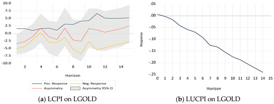
Figure 4.
The cumulative dynamic multiplier of LCPI and LUCPI on LGOLD.
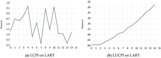
Figure 5.
The cumulative dynamic multiplier of LCPI and LUCPI on LART.
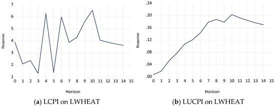
Figure 6.
The cumulative dynamic multiplier of LCPI and LUCPI on LWHEAT.
5.1. The Impact of Inflation on Gold Price
Figure 4a depicts the relationship between CPI shocks and gold price response. The blue line shows a positive correlation, suggesting that gold prices tend to rise during inflation. Conversely, the yellow line indicates a negative correlation, meaning gold prices are likely to fall during deflation.
The overall trend suggests that gold acts as an inflation hedge, with its price increasing more significantly during inflation compared to the decrease during deflation. Figure 4b shows that the cumulative dynamic multiplier is negative for all horizons. This means that a shock to LUCPI will always hurt the price of gold. The effect is most significant in the short term and gradually decreases over the longer term. The CDM signifies that a rise in unexpected inflation may hurt the price of gold. In other words, when inflation increases, the price of gold tends to decrease in the long run. This could be due to rising interest rates making gold less attractive compared to interest-bearing investments or governments selling gold reserves to combat inflation. The impact is most substantial in the short term, with the negative effect gradually weakening. This might be because some investors buy back gold later as a long-term inflation hedge or short-term market fluctuations influencing initial price movements.
5.2. The Impact of Inflation on Art Price
Figure 5a shows that the CDM of LCPI on LART is initially hostile, indicating that an increase in CPI has a negative impact on art prices. This negative effect persists for the first few periods, but gradually diminishes over time. After around the fourth period, the CDM turns positive, suggesting that the impact of CPI on art prices becomes positive. This implies that as CPI persists, art prices may start to rise. Several factors could influence the observed CDM, including art market dynamics, economic conditions, and specific art characteristics. The supply and demand dynamics of the art market play a crucial role. During inflationary periods, investors may turn to art as a store of value, driving up prices. However, if inflation becomes too high, it could dampen overall economic activity, potentially reducing demand for art.
Figure 5b illustrates several key trends regarding the CDM over time in response to a shock. Firstly, the CDM increases steadily over time, indicating that the LUCPI’s impact intensifies as time progresses. This escalation could result from various factors, including the shock exacerbating existing system damage, eroding the system’s inherent resilience, and interacting with other shocks in the system. Secondly, the CDM is higher at longer horizons, suggesting that LUCPI’s long-term repercussions surpass its short-term effects. However, the CDM eventually reaches a plateau at longer horizons, implying that the LUCPI’s long-term impact may encounter limitations or stabilizing factors.
5.3. The Impact of Inflation on Wheat Price
Figure 6a shows that the shock of LCPI to wheat price is positive and increasing over the horizon. This means that the shock has a positive and increasing effect on the wheat price over time. In other words, a shock of CPI may cause the wheat price to increase in the current period and continue to increase in subsequent periods. The CDM for a positive shock is larger than the CDM for a negative shock. This means a positive shock to wheat price has a more significant and more persistent effect than a negative shock.
Figure 6b shows that a shock of LUCPI may have a significant and long-lasting impact on the wheat price. The effect of the shock will be felt for several periods, with the impact gradually diminishing over time. The gradual diminishing effect implies that the market adjusts to the unexpected inflation shock, causing wheat prices to stabilize over time.
The CDM figures shed light on the intricate and ever-changing nature of how shocks ripple through an economic system. While a shock of the CPI, likely due to inflation fluctuations, might directly impact asset prices, the true story is far more nuanced. This initial change triggers a complex chain reaction. The impact on asset prices is not instantaneous and short-lived but instead unfolds over an extended period, with the influence gradually diminishing. This dynamic nature highlights the system’s ability to adapt and find a new equilibrium.
6. A Robust Test for the Long-Run Equilibrium
Table 5 presents the results of a cointegration analysis examining the long-run equilibrium relationship between the natural logarithms of gold price (LGOLD), artistic index (LART), and wheat price (LWHEAT). The intercept (C) is statistically significant at the 1% level for LGOLD and 5% level for LWHEAT, indicating a non-zero constant term in the cointegrating equation.
Table 5.
Cointegrating relationship.
Looking at the coefficients of the independent variables, LUSDIX(-1), the natural logarithm of the US dollar index, has a statistically significant negative impact on LGOLD and LWHEAT at the 1% level. These negative signs suggest that a stronger US dollar is associated with lower gold, art, and wheat prices in the long run. Similarly, LRGDP(-1), the real GDP, has a negative significant coefficient for LGOLD and LWHEAT, implying that lower economic growth might lead to decreased prices for gold and wheat in the long term.
The unexpected inflation, LUCPI(-1), has a negative and statistically significant coefficient for LGOLD at the 10% level but has a minimal effect on LART and LWHEAT. This suggests a potentially weak negative relationship between past unexpected inflation and long-term gold prices. Interestingly, the cumulative changes in past inflation captured by show a positive and significant effect for LGOLD. This indicates a positive relationship between inflation and gold prices during the inflation regime.
A positive coefficient of CPI on art price in the cointegration analysis suggests that, in the long run, art prices tend to increase as inflation rises. This aligns with the concept of art as a potential inflation hedge. As the overall price level increases due to inflation, the value of art might also appreciate, maintaining its purchasing power. However, the negative impact of CPI on art returns reported in Table 4 suggests that the actual returns realized by investors from art investments may not fully compensate for the effects of inflation, resulting in diminished actual returns.
7. Discussion
This study delves into the inflation hedge ability of three distinct assets: gold, art, and wheat, employing a dataset spanning over 31 years. The findings reveal intriguing insights into these assets’ long-run and short-run dynamics in response to various economic factors, particularly inflation, unexpected inflation, real GDP growth, and the US dollar index.
Gold emerges as a notable inflation hedge, particularly in the long run. The negative coefficient for past gold prices suggests a mean-reverting tendency, indicating price adjustments that counteract past increases. However, the result highlights the significance of the US dollar index, with a negative and statistically significant coefficient supporting gold’s role as a hedge against a weakening dollar over the long term. This aligns with the conventional view of gold as a safe haven asset during currency depreciation. Additionally, the result reveals the asymmetric effect of inflation on gold prices, with a positive relationship observed in high inflation regimes. This underscores gold’s function as an inflation hedge, as investors seek to safeguard against erosion of purchasing power during periods of heightened inflation. The short-run analysis further emphasizes the influence of real GDP growth and the US dollar index on gold returns, highlighting the complex interplay between economic factors and gold prices in the short term.
In contrast, the inflation hedge ability of art presents a more insightful picture. While the long-run analysis suggests a weak mean-reverting tendency for art prices, the study uncovers a negative relationship between inflation and art returns. Economic downturns marked by high inflation may dampen consumer discretionary spending on luxury goods like art, diminishing art returns. However, unexpected inflation exhibits a positive and significant association with art returns in the long run, implying art’s potential as an inflation hedge. The short-run analysis reveals a contrasting pattern, with past art price declines associated with lower current art returns. Nevertheless, a positive relationship between inflation and real GDP growth eight periods ago suggests delayed reactions of the art market to economic factors.
Similarly, wheat demonstrates a mean-reverting tendency in the long run, with past price increases counterbalanced by future decreases. While the study finds no statistically significant relationship between wheat prices and inflation, unexpected inflation, or real GDP growth in the long run, the negative coefficient for the US dollar index aligns with gold and art, suggesting a potential long-run negative association between a stronger dollar and wheat prices. The short-run analysis unveils a more intricate picture, with positive and negative coefficients reflecting the dynamic interplay between inflation, real GDP growth, and wheat prices at different points in time.
The error correction analysis confirms a long-term equilibrium relationship between asset prices and economic factors, indicating that deviations from equilibrium are self-correcting over time. The study’s robust model diagnostics further bolsters the estimated coefficients’ reliability and the overall model specification.
Analyzing the cumulative impact of both expected and unexpected inflation shocks across different asset classes highlights their roles as potential inflation hedges. Often regarded as a traditional hedge against inflation, gold exhibits a mixed response. While it tends to appreciate during expected inflation, the impact of unexpected inflation shocks is negative in the long run. This underscores the importance of considering both expected and unexpected inflation scenarios when evaluating gold’s effectiveness as an inflation hedge. In the art market, the findings suggest a more complex relationship. Initial reactions to CPI shocks may be adverse, but art prices tend to rise over time alongside persistent inflation. However, the diminishing returns observed in the long term indicate that the art market’s inflation-hedging capabilities may have limitations. Similarly, wheat prices positively respond to expected inflation, aligning with their short- to medium-term inflation hedge role. While unexpected inflation shocks may disrupt wheat prices temporarily, the market gradually stabilizes, suggesting wheat’s potential as a hedging instrument within a specific time frame.
The findings of this study both align with and diverge from the existing literature on inflation-hedging assets, as outlined in the literature review. Similar to previous studies, this research confirms gold’s established role as a classic inflation hedge, supported by its historical performance and scarcity. However, this study notably contributes in its specialized analysis of art and wheat as inflation hedges. While the literature generally covers commodities broadly, this research explicitly examines wheat. It identifies mean-reverting tendencies over the long term, as well as its intricate interactions with economic growth and inflation. This detailed exploration of agricultural commodities like wheat offers a deeper understanding of their potential as inflation hedges, augmenting broader discussions found in the literature.
8. Conclusions
This study delves into the intricate world of inflation hedging for assets like gold, art, and wheat within the US context (1992–2023). Employing a sophisticated framework (ARDL) that captures nonlinear connections surpasses traditional models and offers a richer understanding of how these assets react to inflation. Furthermore, the study isolates unexpected inflation using a deep learning method.
The findings reveal a multifaceted picture. Gold emerges as a prominent inflation hedge, exhibiting a complex response to inflationary pressures. While it demonstrates a mean-reverting tendency in the long run, its effectiveness as a hedge against expected inflation is tempered by negative reactions to unexpected inflation shocks. The study underscores the role of the US dollar index in shaping gold prices, highlighting its function as a safe asset during times of currency depreciation. In contrast, the inflation hedge ability of art presents a more insightful picture. While it shows potential as a hedge against persistent inflation in the long run, the study reveals a more complex relationship between art prices and economic factors, including unexpected inflation. The diminishing returns observed over time suggest that the inflation-hedging capabilities of the art market may be subject to limitations. Similarly, wheat demonstrates short- to medium-term inflation hedge characteristics, with positive responses to unexpected inflation. Despite temporary disruptions caused by unexpected inflation shocks, the wheat market exhibits a self-correcting mechanism, indicating its potential as a hedging instrument within a specific time frame.
This study builds upon and corroborates established findings in the literature, particularly regarding gold as a reliable inflation hedge. It goes further by offering novel insights into lesser-explored assets such as art and wheat. By employing advanced methodologies like the ARDL framework and LSTM deep learning, the study distinguishes itself from previous research, enabling a more intricate and comprehensive analysis of inflation-hedging dynamics. These methods facilitate a sophisticated exploration of non-linear relationships and unexpected inflation impacts across diverse asset classes, enhancing both theoretical understanding and practical guidance for managing inflation risks in investment and policy contexts.
Funding
This research received no external funding.
Data Availability Statement
This study incorporates price indexes for gold (sourced from the World Gold Council), art (Art Market Research’s innovative valuation approach), and wheat (Macrotrends Data), the Consumer Price Index (CPI) from the International Monetary Fund (IMF), Real Gross Domestic Product (GDP) data from S&P Global, and the US dollar index (Macro-trends Data).
Conflicts of Interest
The authors declare no conflict of interest.
Appendix A
Table A1.
Lag order selection.
Table A1.
Lag order selection.
| Variables | Lag | LR | FPE | AIC | SC | HQ |
|---|---|---|---|---|---|---|
| LCPI (lag = 12) | 0 | NA | 0.041666 | −0.340194 | −0.329660 | −0.336011 |
| 1 | 3009.687 | 1.23 × 10⁻⁵ | −8.469106 | −8.448037 | −8.460739 | |
| 2 | 104.0206 | 9.32 × 10⁻⁶ | −8.745628 | −8.714024 | −8.733077 | |
| 3 | 16.83429 | 8.95 × 10⁻⁶ | −8.785997 | −8.743858 * | −8.769263 | |
| 4 | 0.045463 | 9.00 × 10⁻⁶ | −8.780745 | −8.728071 | −8.759827 | |
| 5 | 0.005804 | 9.05 × 10⁻⁶ | −8.775384 | −8.712176 | −8.750283 | |
| 6 | 2.477986 | 9.03 × 10⁻⁶ | −8.776797 | −8.703054 | −8.747512 | |
| 7 | 1.521271 | 9.04 × 10⁻⁶ | −8.775600 | −8.691322 | −8.742131 | |
| 8 | 0.619494 | 9.08 × 10⁻⁶ | −8.771930 | −8.677118 | −8.734278 | |
| 9 | 5.570886 | 8.99 × 10⁻⁶ | −8.781943 | −8.676596 | −8.740107 | |
| 10 | 2.39 × 10⁻⁵ | 9.03 × 10⁻⁶ | −8.776567 | −8.660685 | −8.730547 | |
| 11 | 14.75203 | 8.72 × 10⁻⁶ | −8.812168 | −8.685752 | −8.761965 | |
| 12 | 10.48765 * | 8.51 × 10⁻⁶ * | −8.836005 * | −8.699055 | −8.781618 * | |
| LGOLD (lag = 12) | 0 | NA | 0.095 | 0.487 | 0.498 | 0.491 |
| 1 | 2284.646 | 0.000 | −5.488 | −5.468 | −5.480 | |
| 2 | 6.679 | 0.000 | −5.501 | −5.469680 * | −5.488302 * | |
| 3 | 2.838 | 0.000 | −5.503 | −5.462 | −5.486 | |
| 4 | 0.149 | 0.000 | −5.498 | −5.447 | −5.478 | |
| 5 | 0.355 | 0.000 | −5.494 | −5.432 | −5.469 | |
| 6 | 0.124 | 0.000 | −5.489 | −5.417 | −5.460 | |
| 7 | 0.002 | 0.000 | −5.484 | −5.401 | −5.451 | |
| 8 | 0.019 | 0.000 | −5.478 | −5.386 | −5.442 | |
| 9 | 0.835 | 0.000 | −5.476 | −5.373 | −5.435 | |
| 10 | 0.000 | 0.000 | −5.470 | −5.357 | −5.425 | |
| 11 | 0.480 | 0.000 | −5.466 | −5.343 | −5.417 | |
| 12 | 16.27057 * | 0.000238 * | −5.505022 * | −5.371 | −5.452 | |
| LWHEAT (lag = 1) | 0 | NA | 0.025 | −0.843 | −0.833 | −0.839 |
| 1 | 1156.464 | 0.001227 * | −3.864982 * | −3.844406 * | −3.856820 * | |
| 2 | 0.967 | 0.001 | −3.862 | −3.831 | −3.850 | |
| 3 | 2.659 | 0.001 | −3.864 | −3.823 | −3.848 | |
| 4 | 0.652 | 0.001 | −3.861 | −3.809 | −3.840 | |
| 5 | 0.238 | 0.001 | −3.856 | −3.794 | −3.832 | |
| 6 | 0.097 | 0.001 | −3.851 | −3.779 | −3.823 | |
| 7 | 0.727 | 0.001 | −3.848 | −3.765 | −3.815 | |
| 8 | 0.175 | 0.001 | −3.843 | −3.750 | −3.806 | |
| 9 | 1.042 | 0.001 | −3.841 | −3.738 | −3.800 | |
| 10 | 0.217 | 0.001 | −3.836 | −3.723 | −3.791 | |
| 11 | 4.333967 * | 0.001 | −3.842 | −3.719 | −3.793 | |
| 12 | 0.017 | 0.001 | −3.837 | −3.704 | −3.784 | |
| LART (lag = 8) | 0 | NA | 0.135 | 0.835 | 0.846 | 0.840 |
| 1 | 1984.255 | 0.001 | −4.354 | −4.333 | −4.346 | |
| 2 | 27.014 | 0.001 | −4.419 | −4.389 | −4.407 | |
| 3 | 9.331 | 0.001 | −4.439 | −4.398 | −4.422 | |
| 4 | 2.265 | 0.001 | −4.440 | −4.388 | −4.419 | |
| 5 | 14.708 | 0.001 | −4.473 | −4.412 | −4.449 | |
| 6 | 21.306 | 0.001 | −4.525 | −4.453 | −4.496 | |
| 7 | 71.534 | 0.001 | −4.710 | −4.627 | −4.677 | |
| 8 | 5.823135 * | 0.000522 * | −4.719896 * | −4.627303 * | −4.683169 * | |
| 9 | 0.314 | 0.001 | −4.716 | −4.613 | −4.675 | |
| 10 | 0.069 | 0.001 | −4.711 | −4.597 | −4.666 | |
| 11 | 0.060 | 0.001 | −4.705 | −4.582 | −4.656 | |
| 12 | 1.825 | 0.001 | −4.705 | −4.571 | −4.652 |
Note: Asterisks (*) denote lag lengths chosen by information criteria (LR, FPE, AIC, SC, HQ). These criteria balance goodness-of-fit and model complexity, with the asterisk indicating the optimal lag for each criterion.
References
- Afham, MSM Khair, Siong-Hook Law, and W. N. W. Azman-Saini. 2017. Is gold investment a safe haven or a hedge for the Malaysian inflation? International Journal of Business and Society 18: 51–66. [Google Scholar] [CrossRef]
- Alagidede, Paul, and Theodore Panagiotidis. 2010. Can common stocks provide a hedge against inflation? Evidence from African countries. Review of Financial Economics 19: 91–100. [Google Scholar] [CrossRef]
- Amenc, Noël, Lionel Martellini, and Volker Ziemann. 2009. Inflation-hedging properties of real assets and implications for asset–liability management decisions. The Journal of Portfolio Management 35: 94–110. [Google Scholar] [CrossRef]
- Arshad, Shaista, Thi Hong Nhung Vu, Too Shaw Warn, and Loke Mei Ying. 2023. The hedging ability of gold, silver, and bitcoin against inflation in ASEAN countries. Asian Academy of Management Journal of Accounting & Finance 19: 121–53. [Google Scholar]
- Attié, Alexander P., and Shaun K. Roache. 2009. Inflation Hedging for Long-Term Investors. International Monetary Fund, Finance Department. Available online: https://www.imf.org/external/pubs/ft/wp/2009/wp0990.pdf (accessed on 25 June 2024).
- Bampinas, Georgios, and Theodore Panagiotidis. 2016. Hedging inflation with individual US stocks: A long-run portfolio analysis. The North American Journal of Economics and Finance 37: 374–92. [Google Scholar] [CrossRef]
- Baral, Srijana, and Bin Mei. 2023. Inflation hedging effectiveness of farmland and timberland assets in the United States. Forest Policy and Economics 151: 102969. [Google Scholar] [CrossRef]
- Bird, Peter J. 1984. Commodities as a hedge against inflation. Applied Economics 16: 855–67. [Google Scholar] [CrossRef]
- Brown, Rob, Richard M. Ennis, Hamza Bahaji, Edouard Van Yen, Brian Bruce, Samveg Patel, Moshe Levy, R. B. Burney, R. N. Killins, A. Murphy, and et al. 2023. Inflation Hedging Tools—What Works and What Doesn’t. The Journal of Investing 32: 24–42. [Google Scholar] [CrossRef]
- Bruno, Salvatore, and Ludwig Chincarini. 2011. A multi-asset approach to inflation hedging fora US investor. The Journal of Portfolio Management 37: 102–15. [Google Scholar] [CrossRef]
- Cheng, Li, Schlanger Todd, and Zhu Victor. 2023. Personalized Inflation-Hedging Strategies. Journal of Portfolio Management 50: 46–57. [Google Scholar]
- Chiang, Thomas C. 2023. Searching for assets to hedge against inflation in the US market. Review of Pacific Basin Financial Markets and Policies 27: 2350029. [Google Scholar] [CrossRef]
- Choi, Sangyup, and Junhyeok Shin. 2022. Bitcoin: An inflation hedge but not a safe haven. Finance Research Letters 46: 102379. [Google Scholar] [CrossRef] [PubMed]
- Ciner, Cetin. 2015. Are equities good inflation hedges? A frequency domain perspective. Review of Financial Economics 24: 12–17. [Google Scholar] [CrossRef]
- Conlon, Thomas, Brian M. Lucey, and Gazi Salah Uddin. 2018. Is gold a hedge against inflation? A wavelet time-scale perspective. Review of Quantitative Finance and Accounting 51: 317–45. [Google Scholar] [CrossRef]
- de Wit, Ivo. 2023. Office Real Estate as a Hedge against Inflation and the Impact of Lease Contracts. Journal of Alternative Investments 25: 81–92. [Google Scholar] [CrossRef]
- Dittmann, Iwona. 2024. The potential of residential property in Poland as an inflation hedge investment. Real Estate Management and Valuation 32: 58–70. [Google Scholar] [CrossRef]
- Eagle, David M., and Dale L. Domian. 1995. Quasi-real bonds: Inflation-indexing that retains the government’s hedge against aggregate-supply shocks. Applied Economics Letters 2: 487–90. [Google Scholar] [CrossRef]
- Essafi Zouari, Yasmine, and Aya Nasreddine. 2024. Housing in the greater Paris area as an inflation hedge? International Journal of Housing Markets and Analysis 17: 837–58. [Google Scholar] [CrossRef]
- Fang, Wen-Shwo, Kuan-Min Wang, and Thanh-Binh T. Nguyen. 2008. Is real estate really an inflation hedge? Evidence from Taiwan. Asian Economic Journal 22: 209–24. [Google Scholar]
- Ghazali, Mohd Fahmi, Hooi Hooi Lean, and Zakaria Bahari. 2015. Is gold a good hedge against inflation? Empirical evidence in Malaysia. Kajian Malaysia: Journal of Malaysian Studies 33: 69–84. [Google Scholar]
- Greene, William H. 2008. Econometric Analysis, 6th ed. Upper Saddle River: Prentice-Hall. [Google Scholar]
- Gyourko, Joseph, and Peter Linneman. 1988. Owner-occupied homes, income-producing properties, and REITs as inflation hedges: Empirical findings. The Journal of Real Estate Finance and Economics 1: 347–72. [Google Scholar] [CrossRef]
- Hochreiter, Sepp, and Jürgen Schmidhuber. 1997. Long short-term memory. Neural Computation 9: 1735–80. [Google Scholar] [CrossRef] [PubMed]
- Iqbal, Javed. 2017. Does gold hedge stock market, inflation and exchange rate risks? An econometric investigation. International Review of Economics & Finance 48: 1–17. [Google Scholar]
- Kuan-Min, Wang, Lee Yuan-Ming, and N. T. T. Binh. 2008. Asymmetric inflation hedge of housing return: A nonlinear vector error correction approach. International Real Estate Review 11: 65–82. [Google Scholar]
- Lee, Chyi L. 2014. The inflation-hedging characteristics of Malaysian residential property. International Journal of Housing Markets and Analysis 7: 61–75. [Google Scholar]
- Liu, Jinan, and Victor J. Valcarcel. 2024. Hedging inflation expectations in the cryptocurrency futures market. Journal of Financial Stability 70: 101205. [Google Scholar] [CrossRef]
- MacKinnon, James G. 1996. Numerical distribution functions for unit root and cointegration tests. Journal of Applied Econometrics 11: 601–18. [Google Scholar] [CrossRef]
- McCown, James Ross, and John R. Zimmerman. 2010. Analysis of the investment potential and inflation-hedging ability of precious metals. In Banking and Capital Markets: New International Perspectives. Singapore: World Scientific Publishing Co., pp. 325–40. [Google Scholar] [CrossRef]
- Nguyen, Binh Thi Thanh. 2023. Can housing investment hedge against inflation? International Journal of Housing Markets and Analysis 16: 1071–88. [Google Scholar] [CrossRef]
- Nguyen, T. Thanh-Binh, and Kuan-Min Wang. 2010. Causality between housing returns, inflation and economic growth with endogenous breaks. Journal of Chinese Economic and Business Studies 8: 95–115. [Google Scholar] [CrossRef]
- Öztürkkal, Belma, and Aslı Togan-Eğrican. 2020. Art investment: Hedging or safe haven through financial crises. Journal of Cultural Economics 44: 481–529. [Google Scholar] [CrossRef]
- Papathanasiou, Spyros, Dimitris Kenourgios, Drosos Koutsokostas, and Georgios Pergeris. 2023. Can treasury inflation-protected securities safeguard investors from outward risk spillovers? A portfolio hedging strategy through the prism of COVID-19. Journal of Asset Management 24: 198–211. [Google Scholar] [CrossRef]
- Pesaran, M. Hashem, and Yongcheol Shin. 1995. An Autoregressive Distributed lag Modelling Approach to Cointegration Analysis. Cambridge: Department of Applied Economics, University of Cambridge, vol. 9514. [Google Scholar]
- Pesaran, M. Hashem, Yongcheol Shin, and Richard J. Smith. 2001. Bounds testing approaches to the analysis of level relationships. Journal of Applied Econometrics 16: 289–326. [Google Scholar] [CrossRef]
- Phochanachan, Panisara, Nootchanat Pirabun, Supanika Leurcharusmee, and Woraphon Yamaka. 2022. Do bitcoin and traditional financial assets act as an inflation hedge during stable and turbulent markets? Evidence from high cryptocurrency adoption countries. Axioms 11: 339. [Google Scholar] [CrossRef]
- Sakurai, Yuji, and Tetsuo Kurosaki. 2023. Have cryptocurrencies become an inflation hedge after the reopening of the US economy? Research in International Business and Finance 65: 101915. [Google Scholar] [CrossRef]
- Salisu, Afees A., Ibrahim D. Raheem, and Umar B. Ndako. 2020. The inflation hedging properties of gold, stocks and real estate: A comparative analysis. Resources Policy 66: 101605. [Google Scholar] [CrossRef]
- Shahbaz, Muhammad, Mohammad Iqbal Tahir, Imran Ali, and Ijaz Ur Rehman. 2014. Is gold investment a hedge against inflation in Pakistan? A cointegration and causality analysis in the presence of structural breaks. The North American Journal of Economics and Finance 28: 190–205. [Google Scholar] [CrossRef]
- Shin, Yongcheol, Byungchul Yu, and Matthew Greenwood-Nimmo. 2014. Modelling asymmetric cointegration and dynamic multipliers in a nonlinear ARDL framework. In Festschrift in Honor of Peter Schmidt: Econometric Methods and Applications. New York: Springer, pp. 281–314. [Google Scholar] [CrossRef]
- Smales, Lee A. 2024. Cryptocurrency as an alternative inflation hedge? Accounting & Finance 64: 1589–611. [Google Scholar] [CrossRef]
- Spierdijk, Laura, and Zaghum Umar. 2015. Stocks, bonds, T-bills and inflation hedging: From great moderation to great recession. Journal of Economics and Business 79: 1–37. [Google Scholar] [CrossRef]
- Taderera, Marimo, and Omokolade Akinsomi. 2020. Is commercial real estate a good hedge against inflation? Evidence from South Africa. Research in International Business and Finance 51: 101096. [Google Scholar] [CrossRef]
- Thi Thanh Binh, Nguyen. 2023. How to Hedge against Inflation Risk in Vietnam. Economies 11: 94. [Google Scholar] [CrossRef]
- Van Hoang, Thi Hong, Amine Lahiani, and David Heller. 2016. Is gold a hedge against inflation? New evidence from a nonlinear ARDL approach. Economic Modelling 54: 54–66. [Google Scholar] [CrossRef] [PubMed]
- Wang, Kuan-Min, Yuan-Ming Lee, and Thanh-Binh Nguyen Thi. 2011. Time and place where gold acts as an inflation hedge: An application of long-run and short-run threshold model. Economic Modelling 28: 806–19. [Google Scholar] [CrossRef]
- Wang, Kuan-Min, Yuan-Ming Lee, and Thanh-Binh Nguyen Thi. 2013. Does gold act as inflation hedge in the USA and Japan. Transformations in Business & Economics 12: 20–43. [Google Scholar]
- Xu, Yingying, Chi-Wei Su, and Jaime Ortiz. 2021. Is gold a useful hedge against inflation across multiple time horizons? Empirical Economics 60: 1175–89. [Google Scholar] [CrossRef]
- Zaremba, Adam, Zaghum Umar, and Mateusz Mikutowski. 2019. Inflation hedging with commodities: A wavelet analysis of seven centuries worth of data. Economics Letters 181: 90–94. [Google Scholar] [CrossRef]
- Zhang, Zhiyuan, Qinglin Sun, and Zichen Wang. 2024. The inflation hedging property of art: Evidence from the US, UK and France. Applied Economics, 1–14. [Google Scholar] [CrossRef]
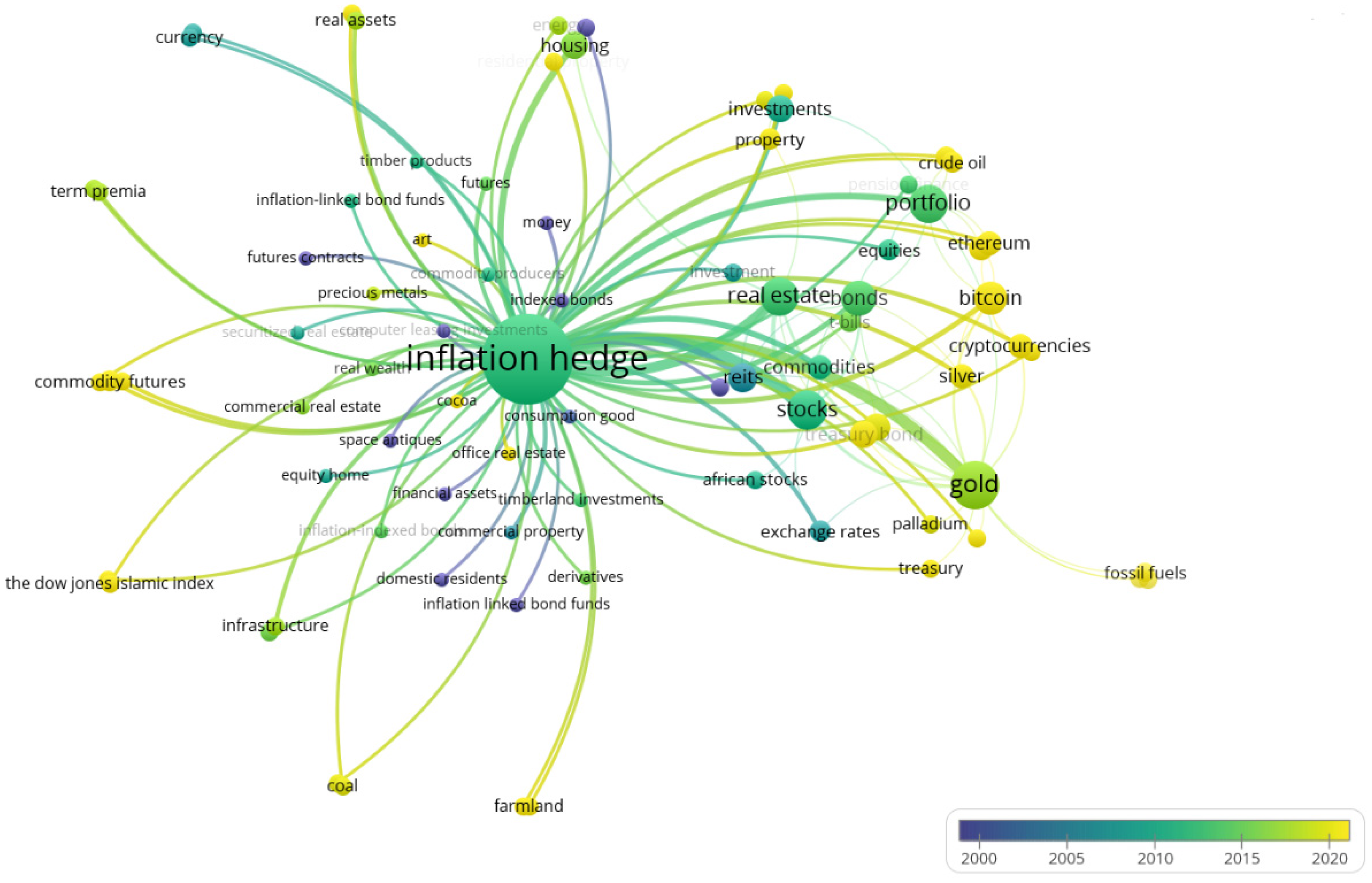

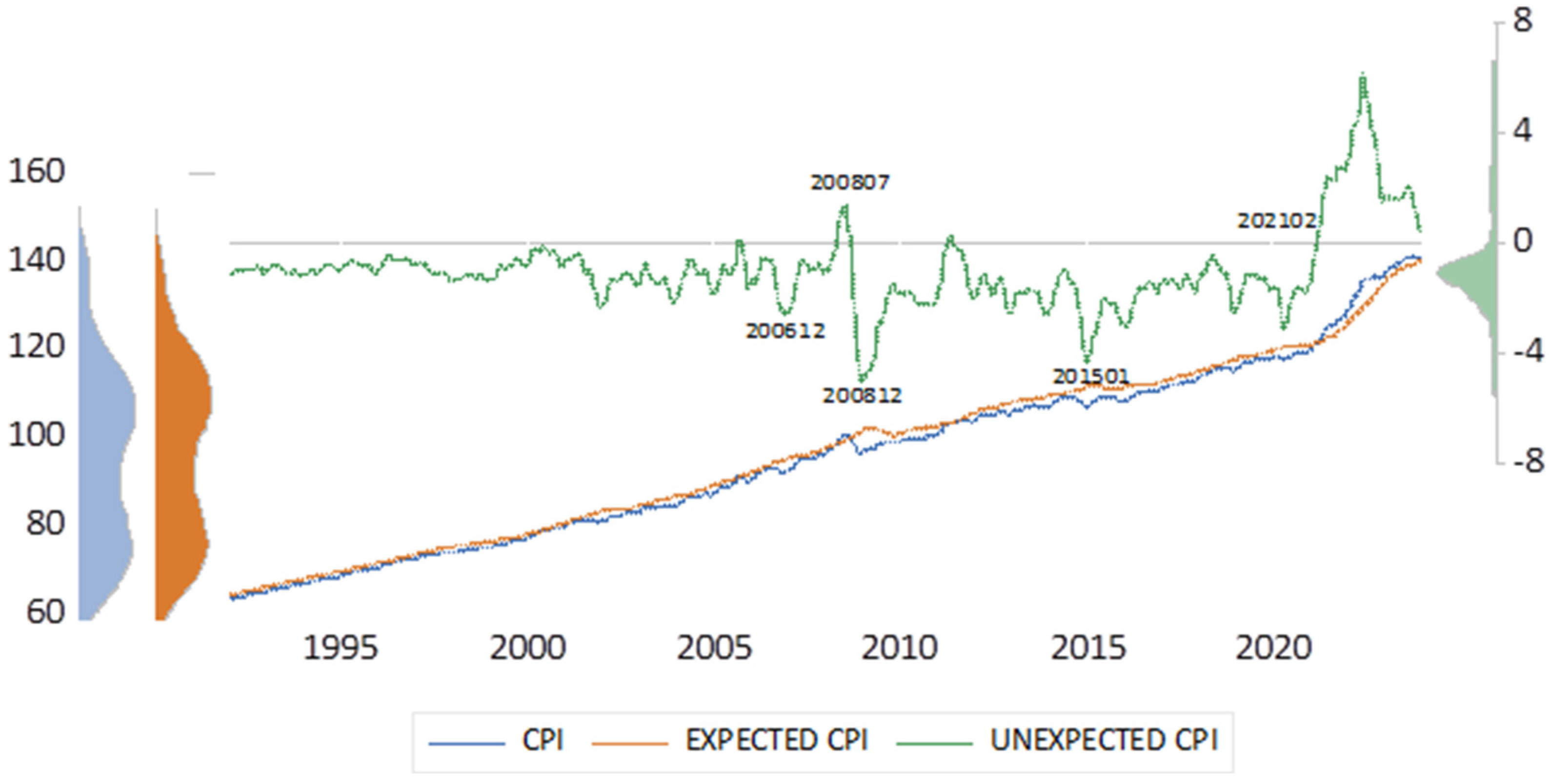
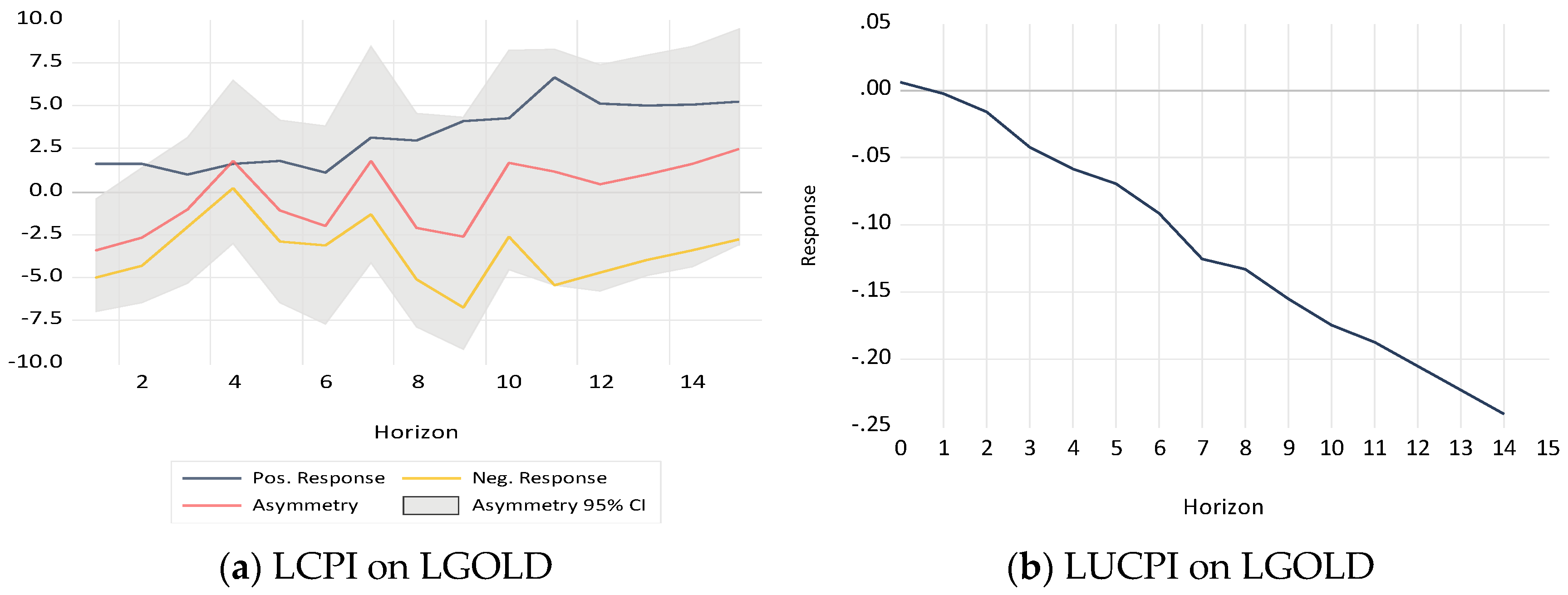

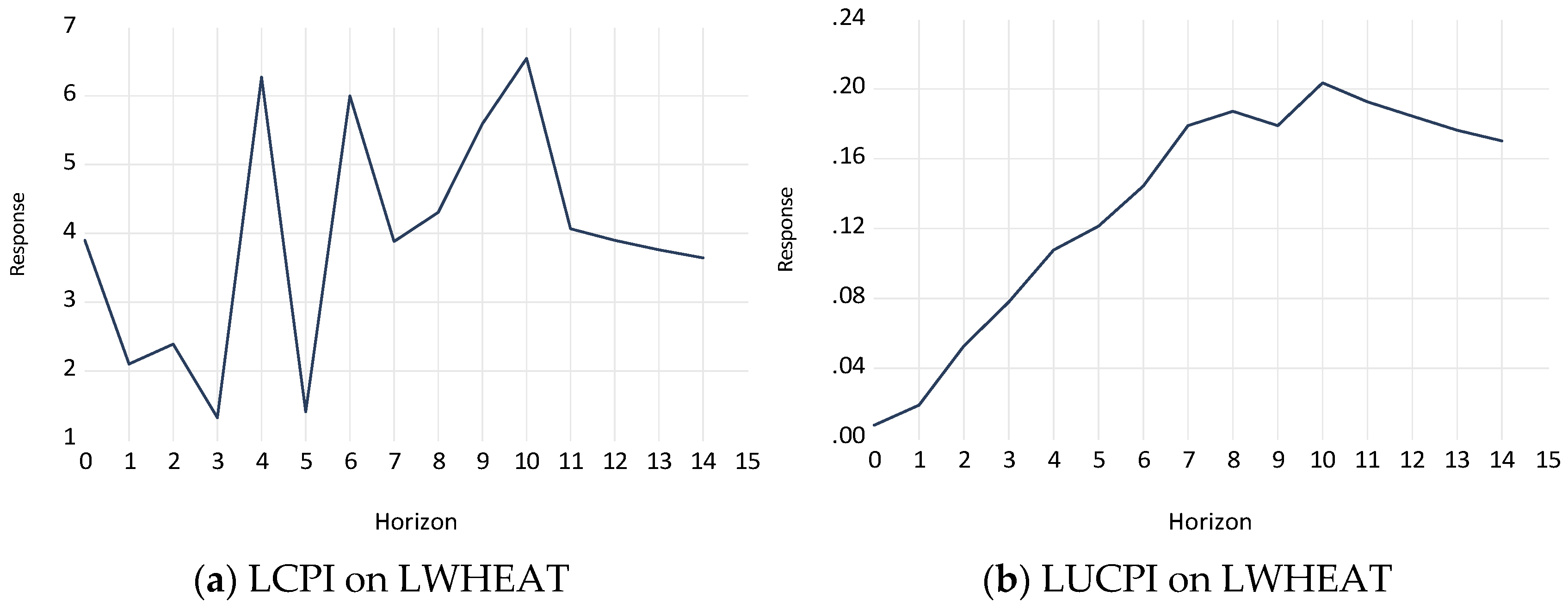
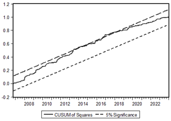
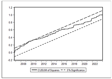
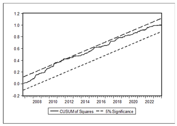
Disclaimer/Publisher’s Note: The statements, opinions and data contained in all publications are solely those of the individual author(s) and contributor(s) and not of MDPI and/or the editor(s). MDPI and/or the editor(s) disclaim responsibility for any injury to people or property resulting from any ideas, methods, instructions or products referred to in the content. |
© 2024 by the author. Licensee MDPI, Basel, Switzerland. This article is an open access article distributed under the terms and conditions of the Creative Commons Attribution (CC BY) license (https://creativecommons.org/licenses/by/4.0/).