Article

The Stability of Trend Management Strategies in Chaotic Market Conditions

by
Alexander Musaev
1 and
Dmitry Grigoriev
2,*
1
St. Petersburg Institute for Informatics and Automation of the Russian Academy of Sciences, 199178 St. Petersburg, Russia
2
Center of Econometrics and Business Analytics (CEBA), St. Petersburg State University, 199034 St. Petersburg, Russia
*
Author to whom correspondence should be addressed.
J. Risk Financial Manag. 2025, 18(1), 33; https://doi.org/10.3390/jrfm18010033
Submission received: 24 October 2024 / Revised: 30 December 2024 / Accepted: 7 January 2025 / Published: 15 January 2025

Abstract

:
This study investigates the stability of trend management strategies under stochastic chaos conditions, with a focus on speculative trading in the Forex market. The primary aim is to evaluate the feasibility and robustness of these strategies for asset management. The experimental setup involves sequential optimization and testing of trend strategies across three EURUSD observation intervals, where each subsequent interval alternates between training and testing roles. Methods include numerical data analysis, parametric optimization, and the use of both conventional and bidirectional exponential filters to isolate system components and improve trend detection. Observations reveal that while trend strategies optimized for specific intervals yield positive results, their effectiveness diminishes on unseen intervals due to inherent market instability. The results show significant limitations in using linear trend-based strategies in chaotic environments, with optimized strategies often leading to losses in subsequent periods. The discussion highlights the potential of integrating trend statistics into multi-expert decision systems, leveraging fuzzy solutions based on fundamental analysis to enhance decision-making reliability. In conclusion, while standalone trend strategies are unsuitable for stable asset management in chaotic markets, their integration into hybrid systems may provide a pathway for improved performance and resilience.

1. Introduction

Proactive control, based on extrapolation computational schemes that detect and identify local trends in observed states of controlled objects, has been the traditional approach (Box et al., 2015; Montgomery et al., 2015; De Gooijer, 2017; Konar & Bhattacharya, 2017; Mills, 2019). Statistical uncertainty has been dampened by transitioning to models of average dynamics using adaptation or robustification technologies (Lauret et al., 2012; Avella Medina & Ronchetti, 2015; Maronna et al., 2019; Musaev et al., 2023a). This approach has yielded satisfactory results when the controlled object’s state changes continuously and with inertia. However, traditional forecasting technologies and proactive management are ineffective in chaotic environments. This is due to the dynamic instability of chaotic processes, where even minor disturbances can lead to unpredictable and radical changes in the state of the controlled object (De Paula & Savi, 2011; Du et al., 2009; Bolotin et al., 2009).
One consequence of dynamic instability is the lack of repeatability for statistically similar observation intervals, violating the condition of repeatability underlying probabilistic–statistical paradigms. This problem has been considered in previous works (Sahni, 2018; Blount & Rush, 2021; Davies, 2018; Musaev, 2011; Musaev et al., 2023b).
This does not mean that statistical data analysis methods are entirely unsuitable. For example, the least squares method always provides an estimate that minimizes the sum of squared deviations. However, in chaotic dynamics, these estimates may be ineffective or even untenable (Feldman, 2019; Musaev et al., 2022; Musaev & Grigoriev, 2022a).
The problem of management in chaotic conditions is particularly acute for information processes not bound by constraints such as continuity and inertia. Examples include financial asset price quotations on electronic capital markets (Inglada-Perez, 2020; Klioutchnikov et al., 2017; Hamidouche et al., 2024; Dwyer & Hafer, 2013). Figure 1 shows EURUSD financial instrument quotation charts and processes formed by smoothing with an exponential filter (Gardner, 1985) with transmission coefficients 0.01 (blue line) and 0.0001 (red line).
The initial process is an oscillatory non-periodic process with many unpredictable local trends, containing signs of chaotic dynamics. However, unlike traditional deterministic chaos models, the observed process contains a pronounced stochastic component that complicates forecasting. Such processes belong to the category of stochastic chaos (Davies, 2018; Musaev, 2011).
The question arises as to how effective traditional trend forecasting technologies and asset management strategies based on these forecasts can be under these conditions. Trend strategies, while effective in detecting linear patterns over short periods, often fail to account for the nonlinearities and stochastic components inherent in chaotic environments. Consequently, such strategies lack robustness, as evidenced by their inconsistent performance across different observation intervals.
In this context, integrating fuzzy-solution-based fundamental analysis alongside trend statistics offers a promising alternative. This hybrid approach leverages the strengths of quantitative trend detection while incorporating qualitative insights from economic indicators, market sentiment, and macroeconomic factors. By employing fuzzy logic to interpret ambiguous or imprecise data, this method provides a more adaptive framework for managing the complexities of financial markets characterized by stochastic chaos. For example, fuzzy logic can refine trend-following strategies by assessing the strength and persistence of detected trends in conjunction with broader market conditions, thus mitigating the shortcomings of purely statistical methods.
The application of fuzzy logic in financial markets has been well-documented. Studies such as (Mangale et al., 2017; Sanchez-Roger et al., 2019) have highlighted its potential in stock market analysis and hybrid prediction models, respectively. These works demonstrate that combining fundamental and technical analyses through fuzzy systems can improve the robustness of forecasting and decision making in volatile markets. By complementing trend statistics with fuzzy logic, we can create multi-expert systems that adapt to the nuances of stochastic chaos, thereby enhancing the stability and performance of asset management strategies.
Given the limitations of traditional trend strategies in chaotic conditions, this article explores the potential of such hybrid methodologies, focusing on the formalization and implementation of proactive management strategies for financial instruments in capital markets.

2. Methods

2.1. Formalization of the Control Problem Under Conditions of Stochastic Chaos

The two-component (Wold, 1938) observation model is used as a basic model for observing the evolution of the state of the observed object:
y k = x k + v k , k = 1 , , n ,
where y k , k = 1 , , n is a time series of samples formed by the monitoring system of the state of the control object. The system component of observations, x k , k = 1 , , n is formed by the sequential filtering of stochastic noise and used in the process of developing control decisions. The noise component of observations v k , k = 1 , , n does not contain useful information and is subject to filtration.
In the Wold model, the system component was an unknown deterministic process, and the noise component v k , k = 1 , , n was a stationary Gaussian process. However, under conditions of stochastic chaos, the nature of these components changes significantly. In this case, the system component x k , k = 1 , , n is an oscillatory non-periodic process with many local trends, indicating that it can be interpreted as a dynamic chaos model (Feldman, 2019). The noise component v k , k = 1 , , n is a non-stationary random process that can be approximately described by a Gaussian model with varying parameters. For example, the variations of the noise component have a non-stationary character, and their correlation and spectral characteristics change significantly over time (Musaev et al., 2023b).
To isolate the system component, any sequential filtering technology can be used. In the simplest case, an exponential filter (Gardner, 1985) can be used for this purpose, determined by the relation
x k = x k 1 + α y k x k 1 , k = 2 , , n ,
with a smoothing coefficient that usually lies within a specific range of values ( 0.001 : 0.1 ) .
In general, isolating a component of a chaotic system from a mixture (1) poses an intricate and ambiguously resolvable problem. The challenge lies in the fact that enhancing the quality of smoothing inevitably results in a bias in the estimate, which manifests as a time delay. This assertion is vividly demonstrated in Figure 1. Consequently, first and second type statistical errors emerge. In this context, these errors represent decisions made about the absence of a trend when it is indeed present (overlooking a trend) and, conversely, decisions made about the presence of a trend when it is absent (false alarm). In the end, these errors invariably culminate in a total loss. To address this, (Musaev et al., 2023c) proposes corrective versions of sequential filtering algorithms that significantly reduce the bias of the estimate while preserving the requisite level of smoothing x k = y ̑ k , k = 1 , , n .
As already mentioned, management in dynamic systems is usually proactive, meaning it is based on a predictive assessment of the system’s state. In some tasks, such as asset management in capital markets, the effectiveness of the management sequence actions u j , j = 1 , , m is entirely determined by the quality of the forecast of the system component x k + τ , k = 1 , , n , where τ is the forecasting interval.
However, making such a forecast in chaotic environments can be extremely difficult due to the instability of the observed process. Even small disturbances from the immersion medium can lead to significant changes in the trajectory of the evolution of the state of the control object.
The overall management efficiency at a selected time interval E f f { U = u j , j = 1 , , m } at the selected time interval k = 1 , , n is estimated as the sum of management quality indicators at each management step. The rule according to which the sequence of controls is selected is
{ U = u j , j = 1 , , m } = S ( x j , θ ) ,
where S x j , θ is called a management strategy, and θ is the management parameters. The effectiveness of proactive management strategies is mainly determined not by the current state of the managed object but by its predicted value x j + τ .
The effectiveness of a management strategy is determined by criteria such as suitability, superiority, or optimality. However, the optimality criterion is rarely used because it is challenging to construct an analytical form of dependence (3) for chaotic processes. The extreme value of the efficiency indicator significantly depends on the specific implementation y k , k = 1 , , n and the reliability of its forecast y ̑ k , k = 1 , , n . Therefore, the suitability criterion is most often used E f f { U } > E f f * , where E f f * is some a priori set threshold value. In particular, if this threshold value is not met E f f * < 0 , then the corresponding management strategy is considered a losing one.
The further specification of the control task in chaotic environments depends significantly on the specifics of the subject area. For example, let us consider a specific example of a management task related to speculative trading in capital markets.

2.2. The Task of Speculative Trading Statement Based on Trend Management Strategies

The task of speculative trading based on trend management strategies involves choosing a control strategy (3) that allows one to determine the sequence of controls u j = ( k i n , k o u t ) j , j = 1 , , m , such that
E f f ( S ) = j = 1 m ( 1 ) c ( y j ( k o u t ) y j ( k i n ) ) p j = m a x .
In this case, the control u j , j = 1 , , m is completely determined by the choice of entry and exit time points ( k i n , k o u t ) j , j = 1 , , m on the market. The value of c = 0 if the position is opened up and c = 1 when the position is opened down. Each control strategy S defines a sequence of controls, i.e., sets the opening and closing moments of a position u j = ( k i n , k o u t ) j , j = 1 , , m and, in some cases, the lot value p j , j = 1 , , m . The strategy is considered winning if E f f S > 0 , taking into account the cost of paying for the spreads of brokerage companies. If the resulting balance at some k-th step turns out to be less than the trader’s deposit D 0 , then this means the completion of the management process with a complete loss.
Trend asset management strategies are based on the assumption that a timely trend detected in the process of changing the value of an asset quote will persist for some unknown time in advance. At each time count k = 1 , , n , the problem of trend detection is solved. When a trend is detected, the market is entered in the direction of the found trend. Exit from the market occurs when pre-set levels of gain (TP—take profit) or loss (SL—stop loss) are reached or based on any other more flexible rules.
Let Δ Y k L , k = ( y k L , , y k ) be a sliding observation window of L samples. The characteristic of a linear trend is its slope coefficient a . To estimate its current value a ̑ k on the sliding observation window Δ Y k L , k , a traditional computational scheme such as OLS can be used. However, given that the value α k is proportional to the increment of a number of observations at a fixed value of the observation window size, the difference value d y ̑ k L , k = y ̑ k y ̑ k L can be used as an estimate of the trend value. To reduce random fluctuation levels, smoothed values formed by a sequential filter of type (2) are used instead of observations themselves. Exceeding the slope of linear approximation’s critical value | d y ̑ k L , k | > d y * indicates the presence of a trend and forms a recommendation to enter the market in the direction of the identified trend.
The values of transmission coefficient α , for smoothing filter, observation window size L and critical value d y * for linear approximation slope are options that are selected a priori by optimizing the training data polygon. Similarly, the best values for TP and SL exit orders can be estimated.

3. Experiments and Results

For the empirical analysis, we used a 10-day subset of one-minute EURUSD quotes drawn from the broader 100-day observation period discussed earlier. This dataset was selected because it represents a variety of market conditions, including both strong trends and sideways movements, offering a robust basis for evaluating the proposed strategies.

3.1. Implementation of a Flexible Trend Management Strategy: Case Study

The TS01 (trend strategy) involves opening a position in the direction of the trend, provided that
| d y ̑ k L , k | > d y * .
The position is closed using protective stop orders TP and SL.
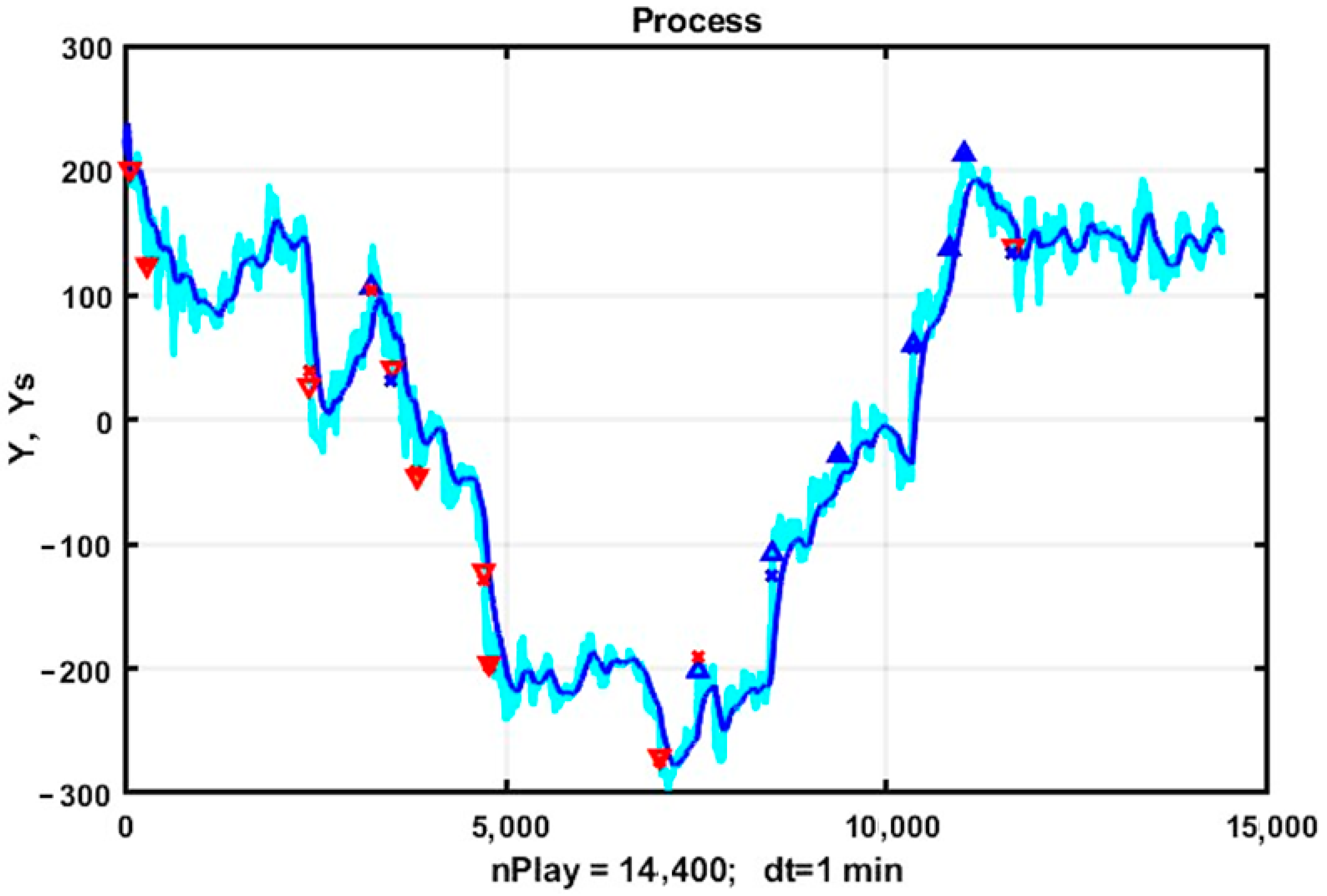
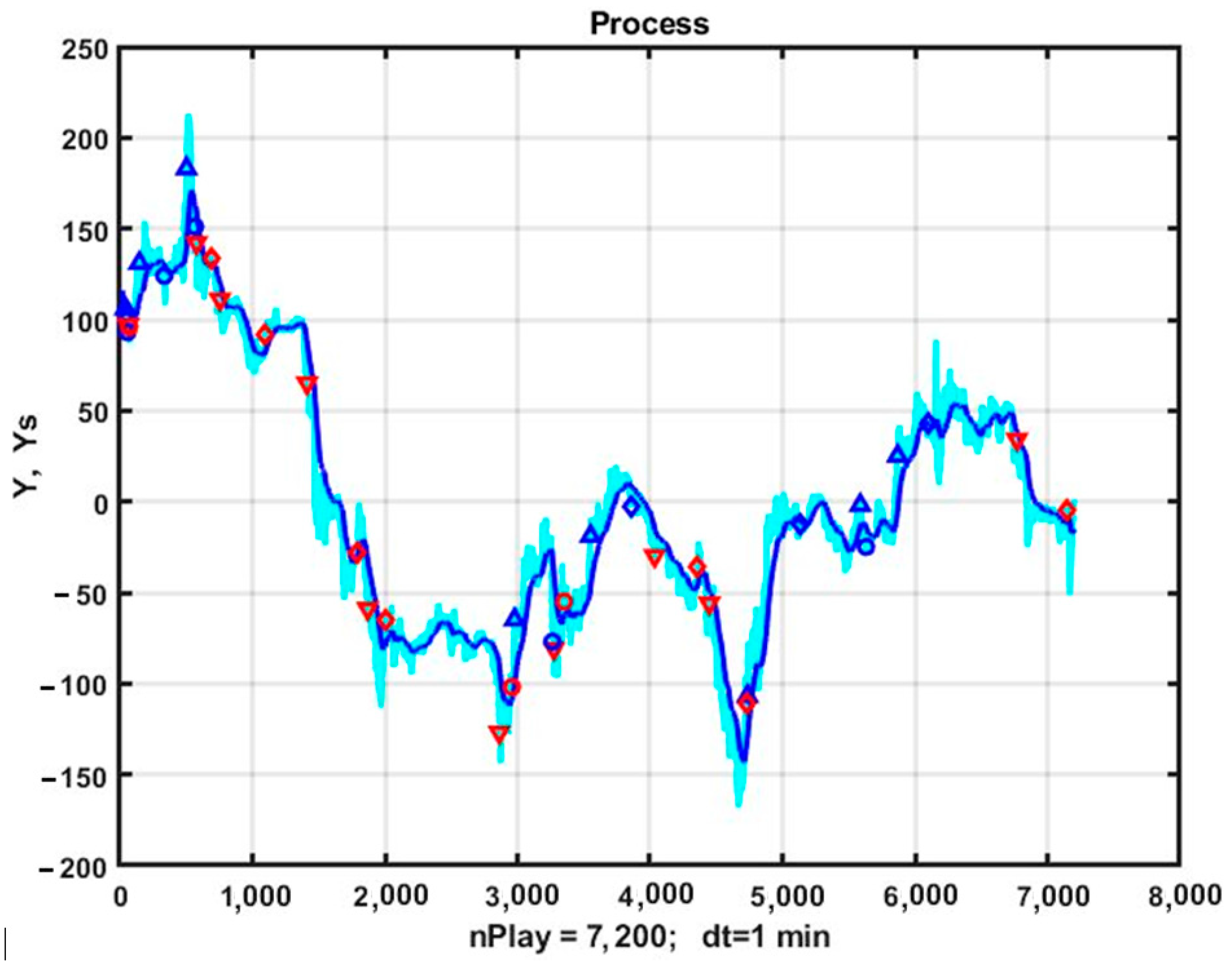
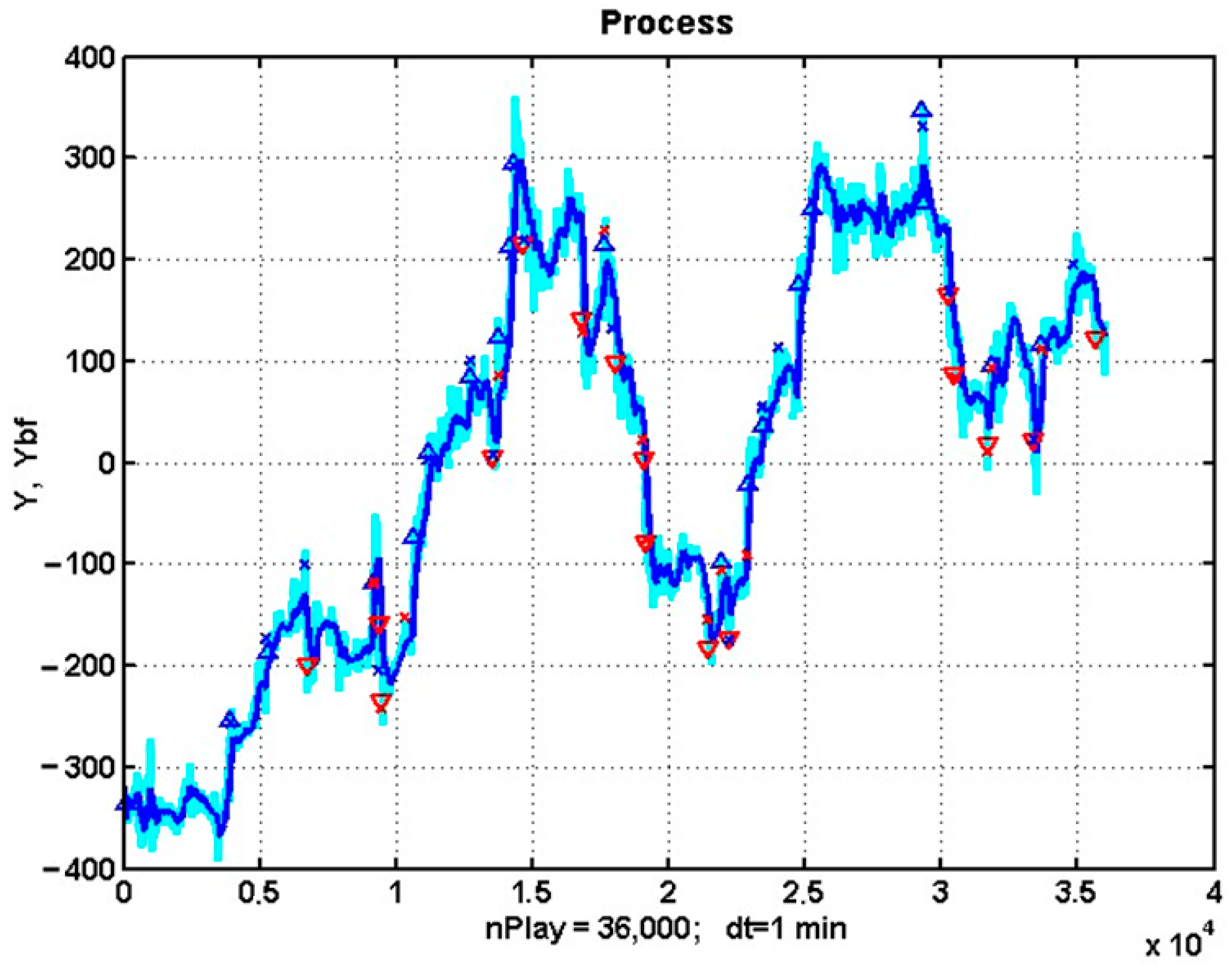
In Figure 2, the vector of optional parameters was chosen to be P = ( α , L , d y * , T P , S L ) = ( 0.01 , 75 , 20 , 75 , 75 ) . The parameter settings were manually selected to demonstrate profitability in markets with pronounced trends. Smoothing coefficients were chosen to reduce noise while maintaining responsiveness. Observation window size (L) was adjusted to capture significant trends without overreacting to short-term fluctuations. Thresholds for trend detection (α) and exit parameters (take profit and stop loss) were optimized to maximize gains during trending market conditions. These values were tailored specifically to showcase the effectiveness of the strategies under favorable market scenarios.
The initial observation series is represented by a sapphire line, while the smoothed values are represented by a blue line. The opening of positions is indicated by triangles of the corresponding orientation (up—blue, down—red), while closing positions are indicated by crosses.
For this realization, the total gain was 133p (points) with a probability of successful (winning) entry into the market of 0.57. A point (point) is understood as a unified unit of change in the value of an asset quotation.
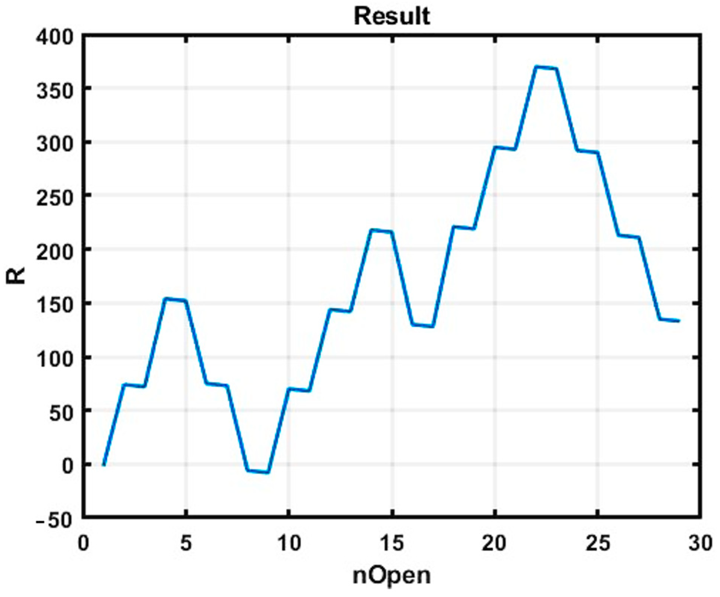
The change in effectiveness for this example presented in Figure 3 shows that the proposed strategy is advantageous if there are sufficiently long-term trends in the value of the asset. In areas with a sideways trend, the trend strategy is losing because trend detection usually precedes a trend reversal.

3.2. Parametric Optimization of the Simplest Trend Strategy

By iterating over the values of the reduced vector of parameters P = ( α , L , d y * ) , while leaving the values T P = S L = 75 , we were able to improve the result by a posteriori optimization. The range and step of parameter changes were α = 0.005 : 0.005 : 0.03 , L = 10 : 10 : 100 , d y * = 10 : 10 : 50 , resulting in 300 variants of combinations of values of the optional parameters of the vector P being tested. The best result was R = 532p with a probability of successful entry into the market of 0.69, achieved at the values of the optional parameters P * = ( 0.01 , 70 , 10 ) . Figure 4 shows an example of the implementation of the TS01 strategy with optimal indicators of optional parameters.
This result allows for further improvement, given that the optimal value of the parameter d y * turned out to be at the lower limit of the selected range of changes in some parameters. In addition, optimization of the values of the TP and SL exit orders is required.

3.3. Preliminary Discussion of the Results

A posteriori optimization for chaotic environments does not always allow for a stable positive effect. Even the optimal solution for the selected observation area may turn out to be a loser in subsequent sections.
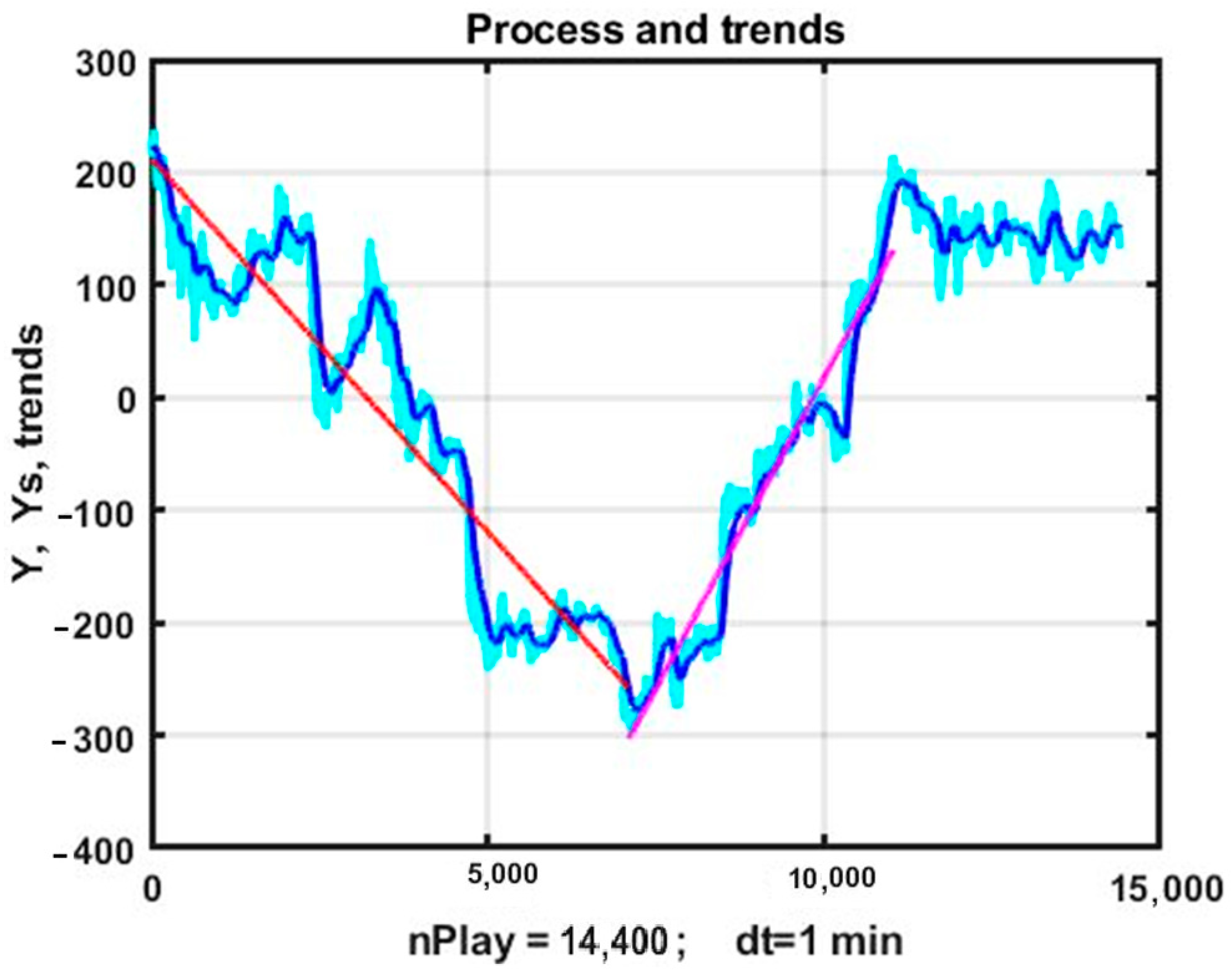
In the Figure 2 and Figure 4, there are two large areas with pronounced trends (see Figure 5), which creates advantageous conditions for the application of trend statistics. However, the remaining observation area (counts 11,040–15,000) is a sideways trend, on which the trend strategy turns out to be losing. The obvious disadvantage of the simplest trend strategy (5) is the mechanistic exit from the market by deterministic TP-SL orders. It would be beneficial to consider a more flexible scheme for exiting the market, based on the features of the evolution of the state of the financial instrument used.

3.4. An Example of the Implementation of a Trend Management Strategy with a Flexible Exit Technology from the Market

The difference between this trend strategy (TS02) and the previous one is that the position is closed (exit from the market), provided that
| d y ̑ k L , k | < d y o .
Thus, the TS02 control strategy is completely determined by the entry rule (6) and the vector of optional parameters P = ( α , L , d y * , d y o ) .
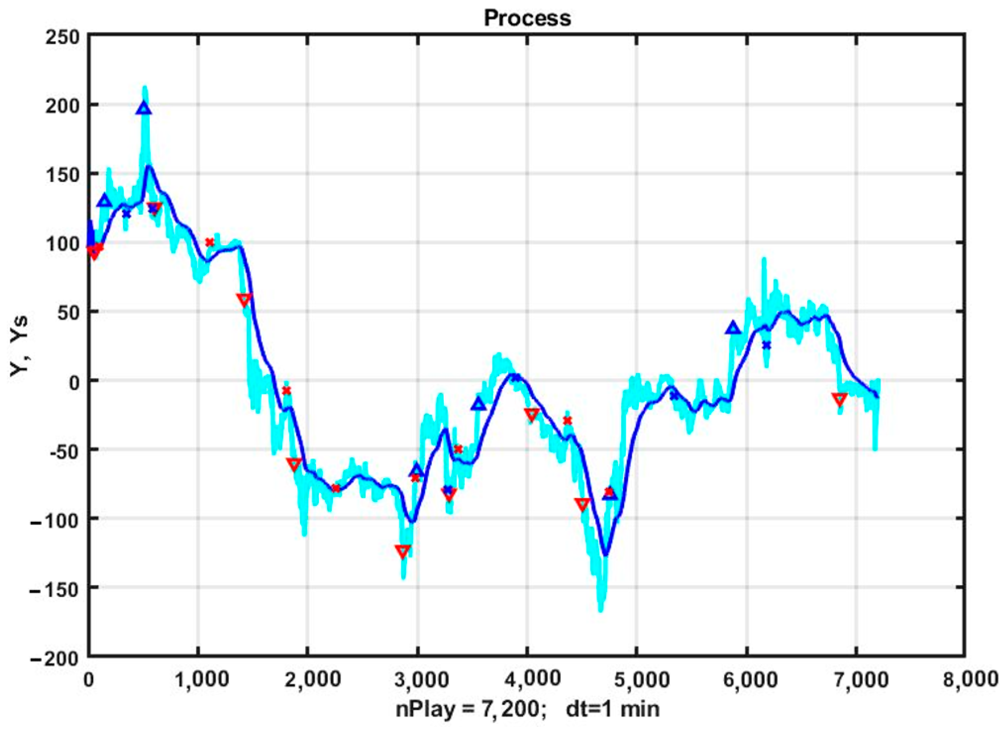
As an example, we use a 5-day observation area with less pronounced trends than in the previous case and define the vector of parameters as P = ( 0.01 , 50 , 8 , 0 ) . Figure 6 shows an example of the implementation of the optimization of the TS02 trend strategy on a 5-day observation interval.
In this example, the application of the TS02 strategy turned out to be a loser, with losses amounting to 25p. and a probability of successful entry into the market of 43%. The reasons for the negative result are due to the fact that the smoothed process always contains an offset that looks like a delay in relation to real observations. Even a small delay is sufficient for the abrupt noise component to turn a positive increment of the smoothed curve into a negative result on real quotation data.

3.5. The Results of the Parametric Optimization of the TS02 Trend Strategy

By iterating over the values of the parameter vector P = ( α , L , d y * , d y o ) with ranges and steps of parameter changes equal to Δ α = 0.005 : 0.005 : 0.03 , Δ L = 10 : 10 : 100 , Δ d y * = 10 : 10 : 50 , Δ d y o = 5 : 1 : 5 , we were able to improve the result. The best result was R = 181p. with a probability of successful entry into the market of 0.56, achieved at the values of the optional parameters P * = ( 0.02 , 40 , 10 , 1 ) . Figure 7 shows an example of the implementation of the TS02 strategy with these optional parameters.
Since the optimal value of d y * = 10 turned out to be equal to the lower limit of its range of change Δ d y * , we chose this range to be Δ d y * = 5 : 5 : 25 and repeated the computational experiment. In this case, the best result was R = 261p. and was achieved with optional parameters P * = ( 0.015 , 20 , 5 , 5 ) . It is interesting to note that changing the allowable range of one parameter changed all optimal values of the vector of parameters for the selected strategy, indicating a significant nonlinearity in the problem being solved.

3.6. Implementation of a Trend Management Strategy with the Detection of Trends on Two Sliding Observation Windows of Different Duration

The choice of the size of the sliding observation window on which the trend is detected carries an obvious contradiction. Reducing the window size leads to increased sensitivity to random variations of the smoothed curve, resulting in statistical errors of the 2nd kind, or “false alarms”. On the other hand, increasing the size of the observation window used to detect a trend leads to a significant delay in decision making to enter the market, which significantly reduces the probability of reaching a winning level.
The difference between this trend strategy (TS03) and the previous ones is that a position is opened while simultaneously exceeding the threshold values of the smoothed curve increments on two sliding observation windows of different lengths:
| d y ̑ k L 1 , k | > d y 1 * & | d y ̑ k L 2 , k | > d y 2 * .
Following the technology of the TS01 strategy, we will close the position by installing orders (TP, SL). Thus, the TS03 control strategy is determined by the rules of entry (7), exit when exceeding the values of orders (TP, SL), and the vector of optional parameters P = ( α , L , d y 1 * , d y 2 * , T P , S L ) .
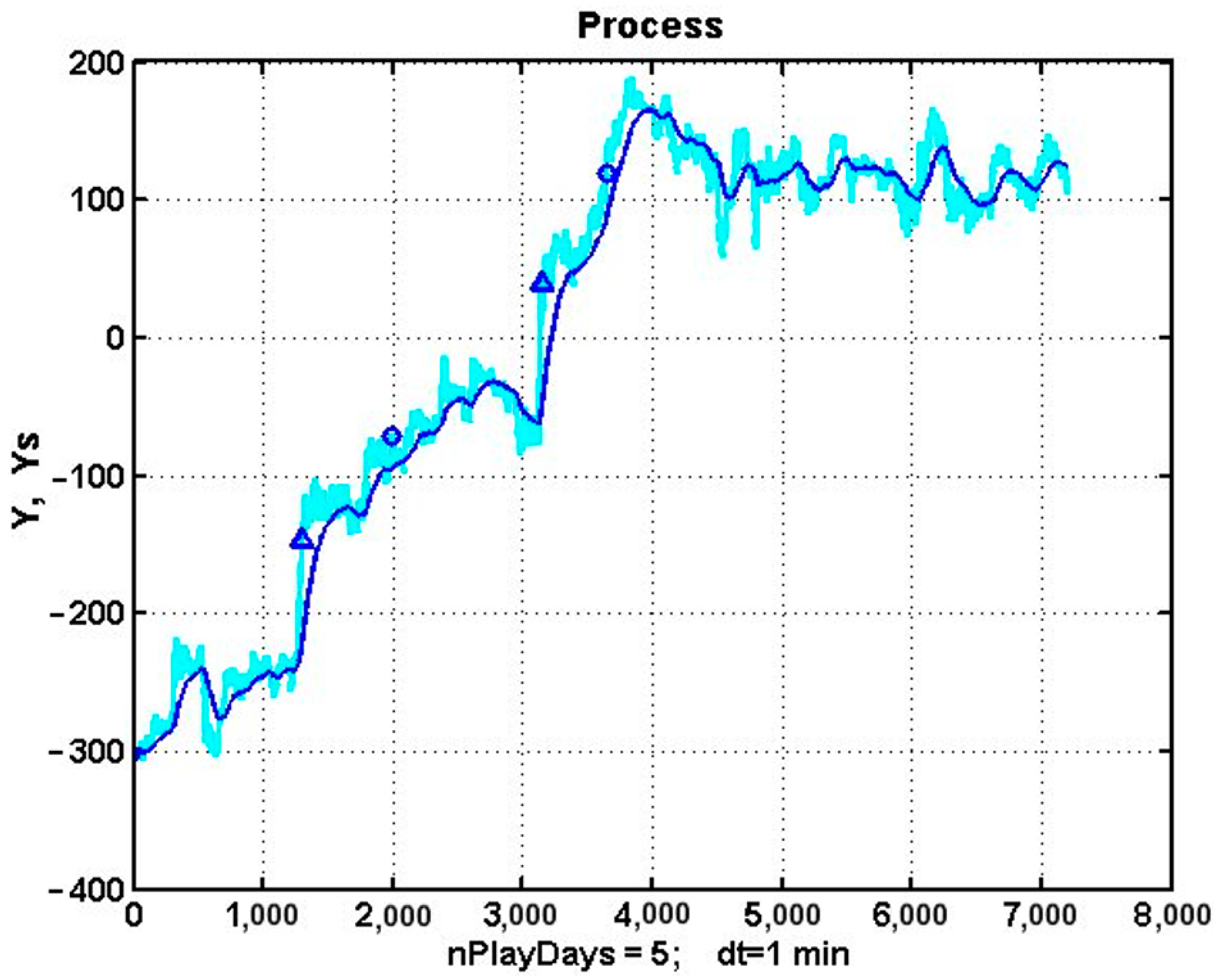
As an example, let us consider the application of the TS03 control strategy with a vector of optional parameters P = ( 0.01 , 50 , 10 , 20 , 75 , 75 ) in a small observation area lasting 5 days. Figure 8 shows the corresponding trading activity.
This strategy retains the disadvantage of the decisive rules of the TS01 and TS02 strategies: opening a position is possible only if condition | d y ̑ k L 1 , k | > d y 1 * is met, allowing for a significant delay in decision making.
Let us also consider parametric optimization of the TS03 strategy by iterating over values of parameter vector P = ( α , L , d y 1 * , d y 2 * , T P , S L ) with ranges and steps equal to
Δ α = 0.005 : 0.005 : 0.025 , Δ L 1 = 10 : 10 : 50 , Δ L 1 = 5 : 3 : 17 , Δ d y 1 = 5 : 5 : 25 , Δ d y 2 = 3 : 1 : 7 .
The best result was R = 384p. and was achieved with optional parameters P* = ( 0.015 , 50 , 17 , 8 , 1 ) . Figure 9 shows an example of implementation for TS03 strategy with optimal indicators for option parameters on the same observation interval as the previous example.
It should be noted that this optimization is a posteriori and carried out according to a previously known observation area. The question remains open as to how stable this result is and whether optimized parameters allow at least a positive result to be preserved at subsequent observation sites.

3.7. An Analysis of the Stability of Optimized Trend Strategies over Long Observation Intervals

To assess the stability of the previously discussed trend-based control strategies, we will carry out sequential optimization and performance evaluation (testing) across three consecutive 100-day observation periods. The first interval was used only for optimization, while the next three intervals played the role of a training polygon (i.e., an optimization interval) and a testing polygon. Performance evaluation was carried out by applying the control strategy optimized at the previous observation site to the observation data at the subsequent interval. The results of the analysis are shown in Table 1, where P* is a vector of optimal parameters for control strategies and R is the effectiveness of applying a strategy with parameters optimized in the previous time interval on a test observation section of 100 days in length. From these results, it appears that the considered trend strategy managers do not have stability and completely lose their effectiveness at the test observation intervals.

3.8. The Problem of Identifying the System Component of a Number of Observations

Trend management strategy technologies are quite effective in areas with pronounced trends in conditions of stochastic chaos. However, for oscillatory modes with weakly expressed trends, the use of trend strategies leads to a losing result.
Parametric optimization of the control strategy allows for a winning result at almost any observation interval. However, this result is not stable and changing the observation interval often leads to a loss. This instability is systemic and is due to the chaotic nature of the data structure.
One factor that significantly affects the effectiveness of trend-based management is the need for consistent smoothing of the initial series of observations. With a large value of the transmission coefficient of the tracking filter, a high level of stochastic volatility remains, leading to a large level of false alarms or erroneous trend detection. Reducing the transmission coefficient improves smoothing quality but leads to a systematic bias in estimation in the form of a time delay. This fact is clearly illustrated in Figure 1.
To reduce this problem’s significance, a bidirectional smoothing method was proposed (Musaev et al., 2023c). Filtering on the selected time window of observation is first carried out in the opposite direction, creating an inverse time delay:
y ̑ k i = y ̑ k i + 1 + α b ( y k i y ̑ k i + 1 ) , i = 1 , , L ,
Then, usual exponential forward filtering is performed on pre-smoothed data:
x j = x j 1 + α f y ̑ j x j 1 , j = k L + 1 , , k .
Using a bidirectional filter allows for significantly reducing displacement with sufficiently high smoothing quality.
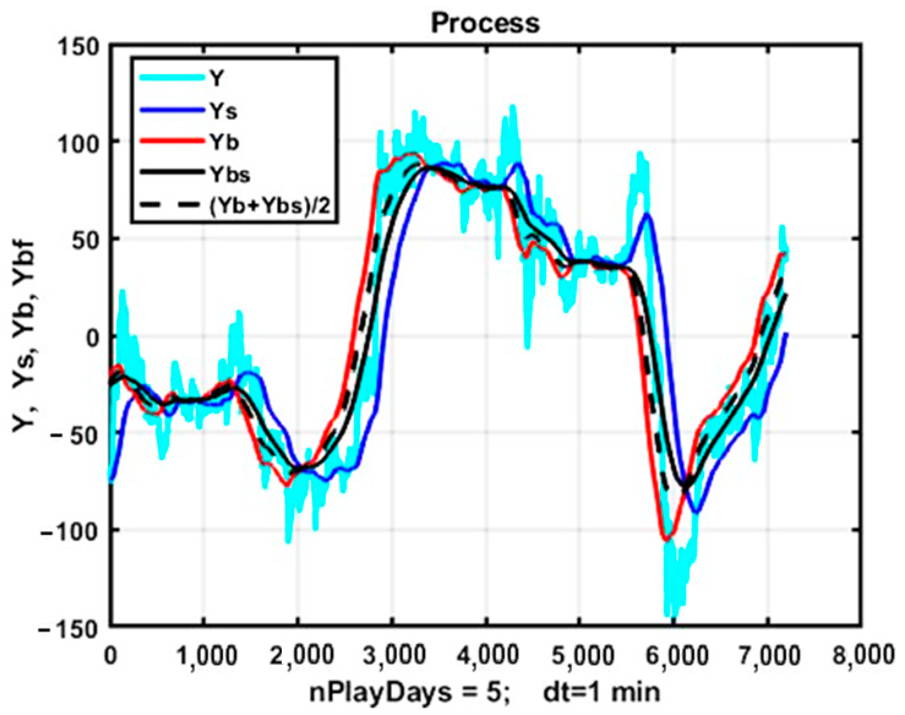
Figure 10 shows a comparison of the filtration quality of exponential and bidirectional filters over a 5-day observation interval. The blue line represents the smoothed curve for the exponential filter (2) Ys with α = 0.005 (blue line) and the bidirectional exponential filter (8–9) with the same value of the transmission coefficient in both directions α b = α f = 0.05 , while the red line Yb corresponds to the result of the inverse exponential smoothing, and the black line Ybs corresponds to the direct inverse exponential smoothing of the Yb process. The black dotted line corresponds to the averaging (Yb + Ybs)/2.
It is evident that using a bidirectional filter significantly reduces the amount of displacement while maintaining a high smoothing quality. For this example, the estimate of the standard deviation (SD) of the residuals of the exponential filter was s(Y, Ys) = 28.6, and the SD of the bidirectional filter was s(Y, Ybf) = 20.2.
In practice, a complete bidirectional recalculation of the smoothed values with a return to the first sample is redundant. It is sufficient to perform a reverse recalculation on a certain sliding observation interval with a length of L samples. Additionally, the best smoothing results according to the criterion of the mean square error d 2 = σ 2 + b 2 , where σ is the SD, and b is the offset of the formed estimate, are usually achieved for different values of the transmission coefficients when smoothing in reverse and forward directions ( α b , α f ) .
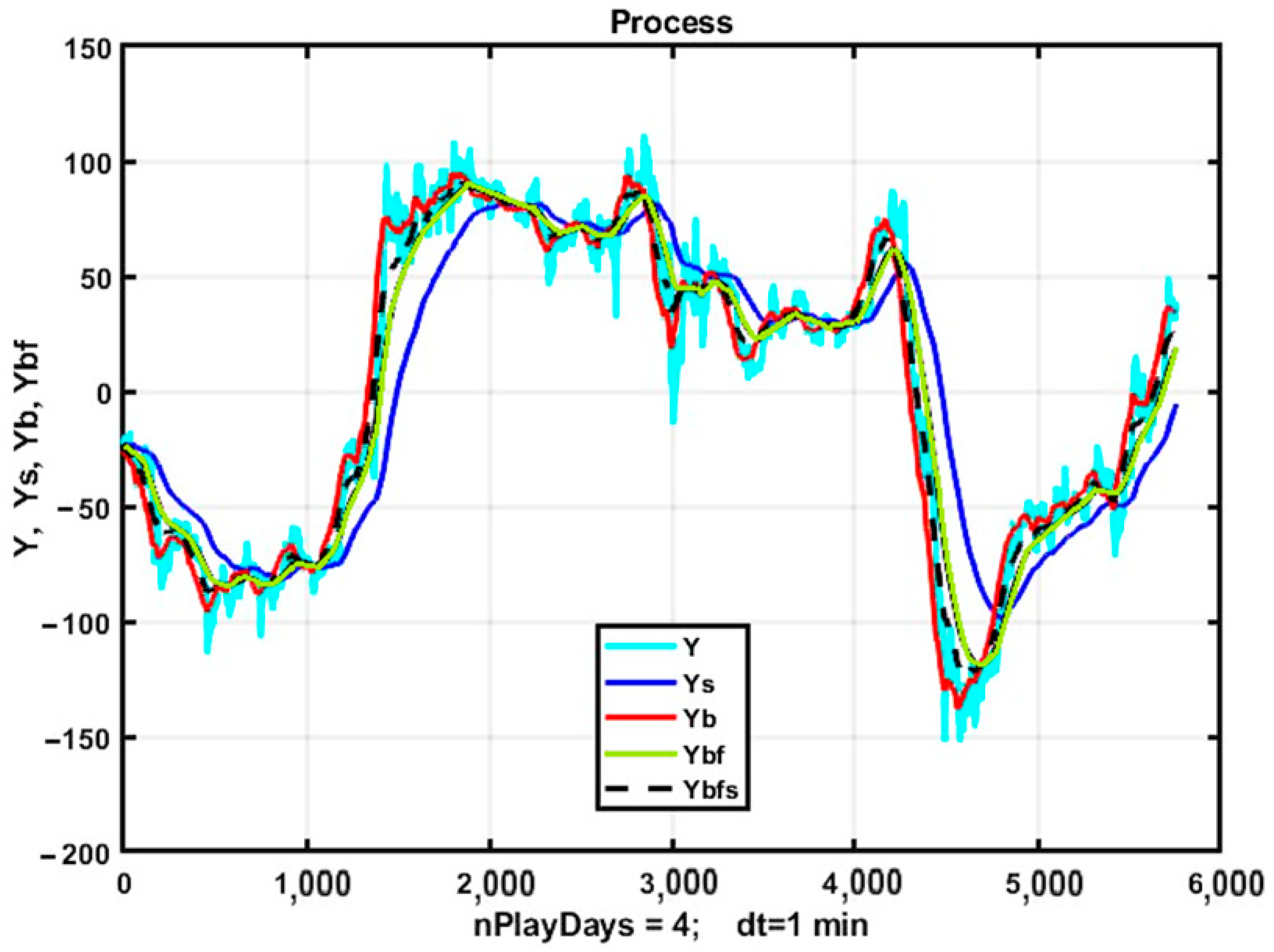
Figure 11 shows the results of filtering an exponential filter (2) with a transmission coefficient α = 0.005 (blue line) and a bidirectional exponential filter with transmission coefficients α b = 0.02 , α f = 0.01 over an observation interval of 4 days with a limitation on the number of reverse smoothing samples by a sliding observation window of L = 100 min. For this example, the SD of the residuals of the exponential filter was s(Y, Ys) = 30.5, and the SD of the bidirectional filter was s(Y, Ybf) = 10.8.
It should be noted that to compare the quality of system component allocation, unlike in traditional tasks of filtering random noise observations, using SD as an indicator is not entirely accurate. For instance, the best result s(Y, Ys) = 0 would correspond to complete absence of filtering, i.e., Ys = Y. Therefore, it is advisable to evaluate the quality of system component allocation based on the terminal task of evaluating control algorithm quality, which consistently includes various options for sequential data filtering.

3.9. Analysis of the Effectiveness of Trend Strategies When Using a Bidirectional Exponential Filter

Let us consider the problem of using the simplest trend strategy in combination with an algorithm for allocating a system component based on a bidirectional exponential filter. Figure 12 and Figure 13 show graphs of the results of applying the TS01 control strategy on the same observation interval with a duration of 25 days when using an exponential filter (on the left) with a transmission coefficient of α = 0.01 and a bidirectional exponential filter with transmission coefficients α b = 0.02 , α f = 0.01 and a sliding smoothing window of length L = 100 samples (right).
The use of a bidirectional filter in this example allowed us to gain 296 p. with a probability of successful market entry P = 0.55. For comparison, using the same control strategy with a conventional exponential filter in the same observation area resulted in 147 p. with a probability of successful market entry P = 0.53.
However, this result can be only a special case. To increase objectivity, sequential parametric optimization of both filters on the same observation should be conducted. This process involves adjusting transmission coefficients and key parameters to compare their performance under identical conditions. Testing on diverse market scenarios, including high volatility and sideways trends, as well as out-of-sample datasets, is essential to evaluate robustness.

4. Discussion

The use of a bidirectional algorithm for highlighting the system component of a series of observations can significantly improve the efficiency of management based on trend strategies. However, even this technology does not allow for a radical improvement in the stability and efficiency of this type of control over long observation intervals. To confirm this conclusion, we will conduct a numerical experiment with sequential parametric optimization of the TS01 strategy and its testing on a subsequent time interval. The corresponding results are presented in Table 2. Here, the duration of the optimization and testing sections is the same and amounts to 144,000 counts (100 days). The values of the optimal parameters P * = [ α b , α f , L , d Y t ] , the results of optimization R* and testing R t , as well as the frequency of successful market entries P+ in the testing area are presented in rows 3, 4, and 5 of Table 2. The results shown in the table clearly indicate the instability of the effectiveness of the trend strategy, including with improved system component allocation technology based on bidirectional exponential smoothing. Similar results are demonstrated by management strategies TS2 and TS03.
The resulting conclusion is expected given the low predictability of processes generated by dynamic chaos. An additional factor that worsens forecast quality is a random component formed by a large number of uncertain influencing factors. In other words, currency instrument quotation dynamics should apparently be attributed to stochastic chaos. This issue is discussed in more detail in (Musaev et al., 2023b). Nevertheless, trend strategies can be widely used as components of multi-expert decision-making systems (MES) (Musaev & Grigoriev, 2022b). We will consider this possibility in the next section.

4.1. Application of Trend Strategies with Multi-Expert Decision-Making Systems

As an illustrative example, let us consider a system for forming control decisions based on the current recommendations of two program experts (PE). The first expert, PE1, forms a fuzzy predictive solution that determines the possibility and direction of a trend in the predicted trading area. The solution is formed by choosing one of the digital values from the set of solutions D = {−2, −1, 0, 1, 2}, each corresponding to fuzzy conclusions {strong negative trend, weak negative trend, absence of a pronounced trend (flat), weak positive trend, strong positive trend}. Fuzzy conclusions are formed by processing analytical forecasts formed by specialists in the field of fundamental analysis of the current economic situation and posted on financial and brokerage company websites on the Internet. Data processing is carried out by implementing algorithms for automatic content detection from text messages. The general method of identifying content is based on text mining algorithms described in (Hotho et al., 2005; Chauhan & Tyagi, 2019; Mahesh et al., 2016). The second expert advisor is based on one of the trend strategies described above, but the decision is made only when the trend possibility is confirmed by the first expert. Let us consider a variant of constructing the described MES with two experts, in which the first expert forms an overall assessment of market sentiment (taking into account a possible error caused by incorrect content extraction from a text message) with a probability of 70%. The second expert implements solutions based on the TS01 control strategy, and a bidirectional exponential filter with parameters α b = 0.02 , α f = 0.01 , L = 100 is used to identify the system component. The decision of the second expert is accepted for execution only in cases when it coincides with the prognostic assessment of the first experiment. So, for example, entry into the market in an upward direction (growth of quotations) is carried out when condition (10) is met:
d y ̑ k L , k > d y * & ( D = 1 V D = 2 ) .
In the opposite direction, entry into the market is carried out under condition
d y ̑ k L , k < d y * & ( D = 1 V D = 2 ) .
If the expert predicts a flat D = 0 , no entry into the market based on a trend strategy is made.
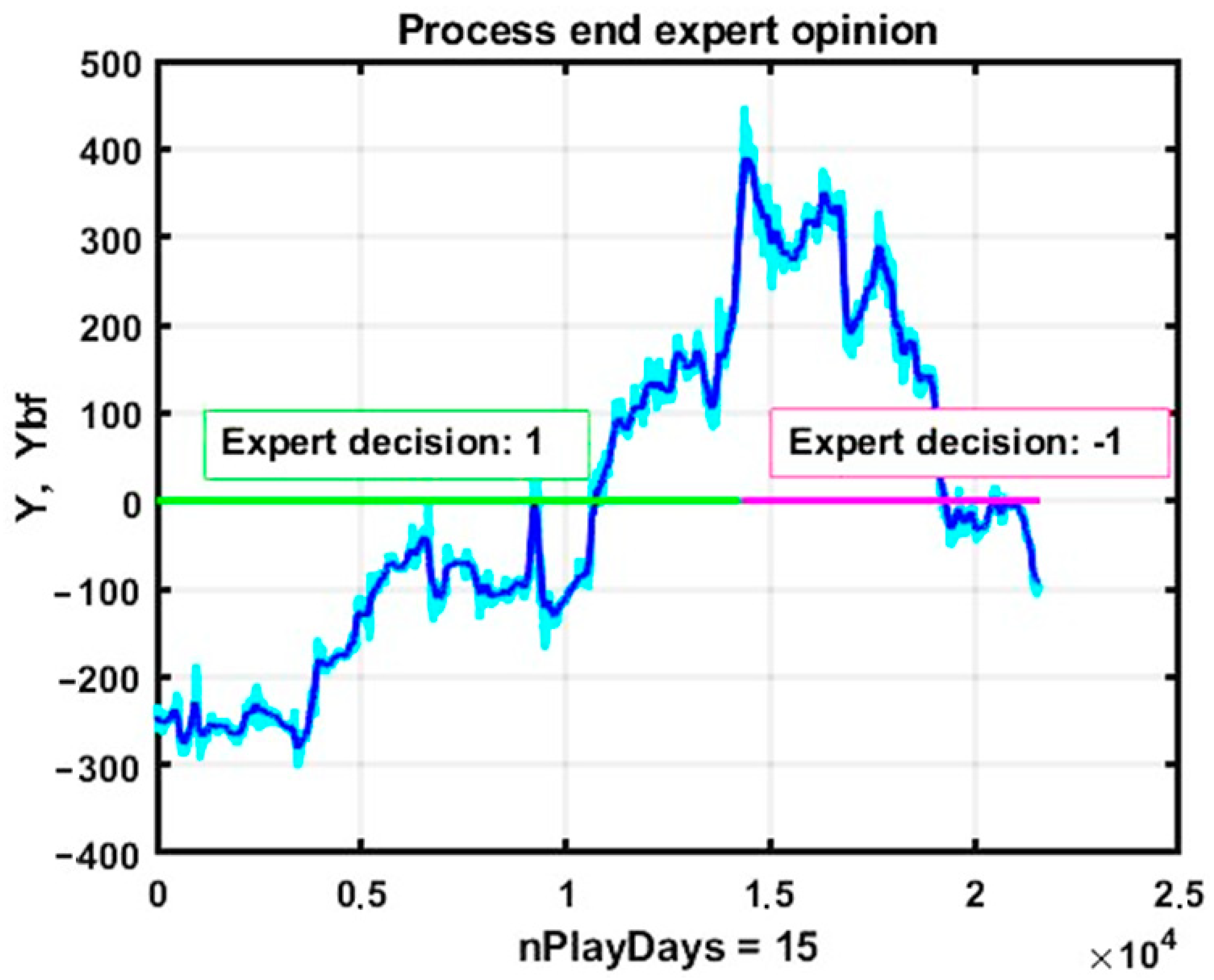
Figure 14 shows an example of a predictive assessment of observed process dynamics by an expert analyst based on fundamental analysis and expected news flow. The expert predicted an increase in financial instrument quotes within 15 days and then their decline within 10 days. The expert caught only the general direction and did not take into account two or three areas with sideways trends or identify areas with rapid changes in quotations.
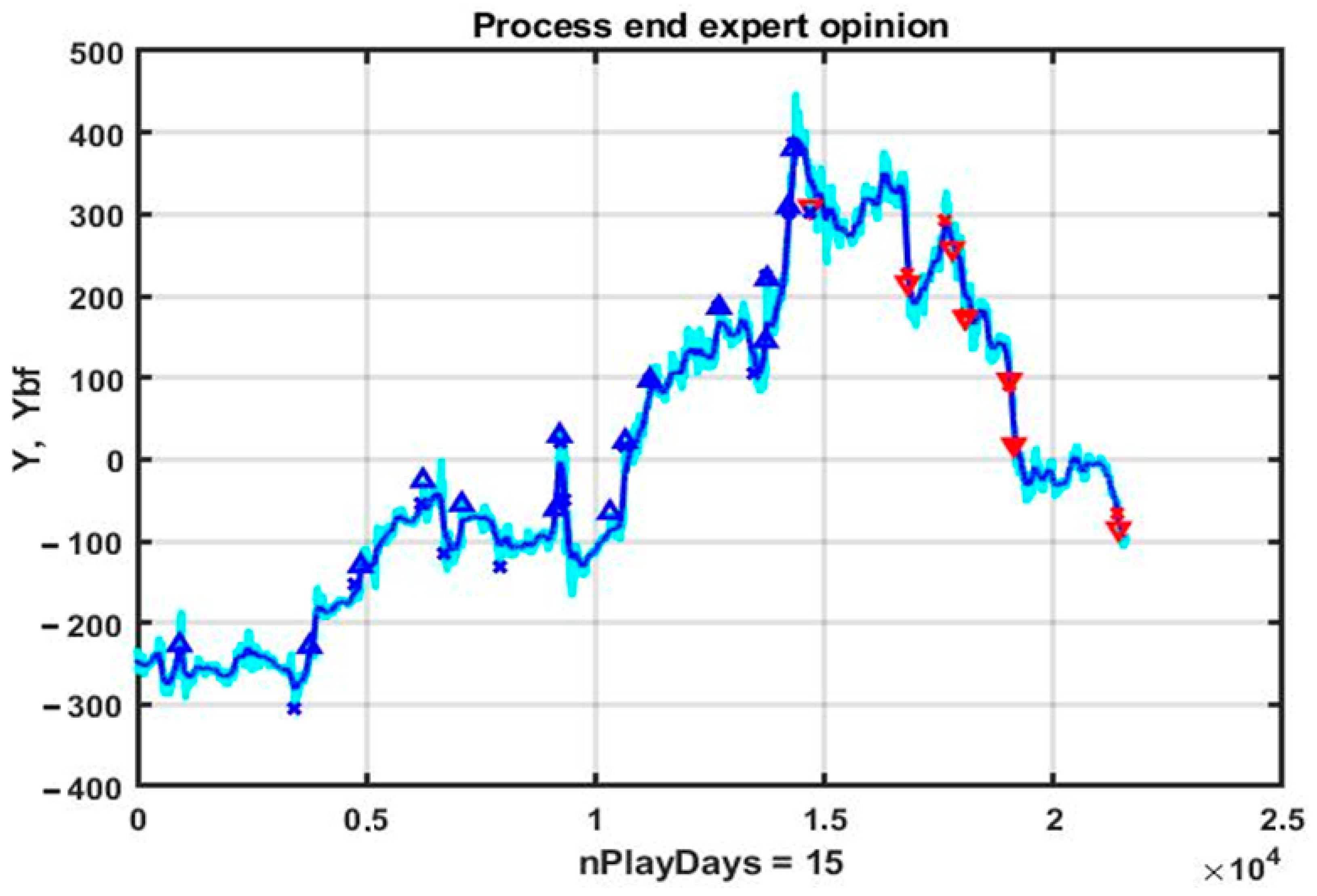
The use of MES technology that includes the TS01 trend strategy algorithm allowed for gaining 524 p. with a probability of successful market entry P = 0.64. The use of this technology on a 25-day plot corresponding to Figure 14’s trading process is shown in Figure 15. For comparison, using TS01 strategy without taking into account expert forecast resulted in only 274 p. with a probability of successful market entry P = 0.58. Of course, this example is only a special case. However, statistical numerical analysis for various observation sites showed that using MES technology with trend strategies allows for obtaining stable positive results provided that experts can correctly predict market mood with at least 60–65% probability.

4.2. Comparison with Contemporary Approaches in Trend-Following Strategies

The findings of this study align with and extend the work of recent studies in trend-following strategies and chaotic market dynamics. (Ayed et al., 2016) highlighted the robustness of trend-following strategies utilizing cross moving averages under parameter misspecifications. Their research emphasized the superior stability of these strategies compared to optimal models in cases where parameter tuning is imprecise. This complements our observations, as the instability of optimized parameters across different intervals in chaotic environments is evident in our results. Incorporating cross moving averages could further enhance the robustness of trend-following strategies.
(Lempérière et al., 2014) conducted a comprehensive historical analysis of trend-following strategies over two centuries, concluding that trends are one of the most statistically significant market anomalies. They demonstrated that while these strategies are effective in stable markets, they often falter in chaotic or high-volatility conditions. This observation reinforces the systemic instability identified in our study, particularly the inability of optimized strategies to generalize beyond the intervals they were trained on.
(Navarro-Barrientos, 2008) explored adaptive strategies in periodic environments, showing that flexibility in trading models, especially those integrated with technical analysis, can significantly improve outcomes. This insight aligns with our recommendation for hybrid approaches that combine trend-following strategies with adaptive components, such as expert systems or machine learning models, to address unpredictable market fluctuations.
(Mansurov et al., 2023) provided a theoretical framework for understanding the interactions between fundamentalist, trend-following, and contrarian trading strategies. Their model revealed that these interactions often produce complex dynamics, including chaotic price behaviors. This supports our finding that the chaotic nature of market data inherently limits the predictive accuracy of trend-following strategies and necessitates more comprehensive modeling approaches.
These studies emphasize the critical need for robustness and adaptability in trend-following strategies, particularly in chaotic market conditions. Future research could explore the integration of cross moving averages, adaptive strategies, and advanced hybrid models to improve the stability and efficiency of trend-following techniques in financial markets.

5. Conclusions

Predicting situations based on trend statistics is a traditional and effective method for proactive management in inertial environments. However, for nonlinear information processes lacking significant inertia, forecasts based on prolongation are generally incorrect. This is especially true for processes with signs of dynamic chaos, such as non-periodic fluctuations and heteroskedasticity. These signs are characteristic of series of observations formed by monitoring market asset states.
This article shows that various control strategies based on trend statistics allow for a posteriori parametric optimization and the possibility of obtaining a winning result on a selected time interval. However, this result lacks stability, and algorithms that win in one time interval may lose in subsequent intervals. Thus, management strategies based on detecting and prolonging linear trends are unsuitable for asset management in conditions of market chaos.
Despite this, trend statistics can still be used as an element of a multi-expert system for forming management decisions. In combination with a system for generating fuzzy solutions based on fundamental analysis, trend statistics can yield significant gains. The limited volume of this article did not allow us to cite research materials on natural development of considered technologies based on nonlinear trend strategies. This will be addressed in the next publication.
Another important area of research is studying trend management strategies for multidimensional non-stationary processes. Under certain conditions, the multidimensionality of mutually correlated processes can act as a regularizing factor and increase extrapolation forecast effectiveness. This has been justified in works devoted to regression and precedent forecasting technologies in unstable immersion environments (Musaev et al., 2022).

Author Contributions

Conceptualization, methodology, validation, writing, A.M.; review and editing, investigation, programming, visualization, administration, scientific discussions, supervision, funding acquisition, D.G. All authors have read and agreed to the published version of the manuscript.

Funding

Alexander Musaev’s research for this paper was supported by a grant from the Russian Science Foundation (Project No. 24-19-00823). Dmitry Grigoriev’s research for this paper was supported by Saint-Petersburg State University, project ID: 103905424.

Institutional Review Board Statement

Not applicable.

Informed Consent Statement

Not applicable.

Data Availability Statement

The source of data—Finam.ru (https://www.finam.ru/, accessed on 24 November 2024).

Acknowledgments

The authors are grateful to participants at the Center for Econometrics and Business Analytics (ceba-lab.org, CEBA) seminar series for helpful comments and suggestions.

Conflicts of Interest

The authors declare no conflicts of interest.

References

  1. Avella Medina, M., & Ronchetti, E. (2015). Robust statistics: A selective overview and new directions. Wiley Interdisciplinary Reviews: Computational Statistics, 7(6), 372–393. [Google Scholar] [CrossRef]
  2. Ayed, A. B. H., Loeper, G., & Abergel, F. (2016). Robustness of mathematical models and technical analysis strategies. arXiv, arXiv:1605.00173. [Google Scholar]
  3. Blount, K. A., & Rush, L. (2021). Chaos theory (Vol. 3). Crush. [Google Scholar]
  4. Bolotin, Y., Tur, A., & Yanovsky, V. (2009). Chaos: Concepts, control and constructive use. In E. Schöll, & H. G. Schuster (Eds.), Springer series in synergetics (pp. 19–34). Springer. [Google Scholar]
  5. Box, G. E., Jenkins, G. M., Reinsel, G. C., & Ljung, G. M. (2015). Time series analysis: Forecasting and control. John Wiley & Sons. [Google Scholar]
  6. Chauhan, H., & Tyagi, H. (2019). Text mining techniques for extraction and retrieval information in research process. International Journal of Research in Electronics and Computer Engineering, 7(2), 2693–700. [Google Scholar]
  7. Davies, B. (2018). Exploring chaos: Theory and experiment. CRC Press. [Google Scholar]
  8. De Gooijer, J. G. (2017). Elements of nonlinear time series analysis and forecasting (Vol. 37). Springer. [Google Scholar]
  9. De Paula, A. S., & Savi, M. A. (2011). Comparative analysis of chaos control methods: A mechanical system case study. International Journal of Non-Linear Mechanics, 46(8), 1076–1089. [Google Scholar] [CrossRef]
  10. Du, J., Huang, T., & Sheng, Z. (2009). Analysis of decision-making in economic chaos control. Nonlinear Analysis: Real World Applications, 10(4), 2493–2501. [Google Scholar] [CrossRef]
  11. Dwyer, G. P., & Hafer, R. W. (Eds.). (2013). The stock market: Bubbles, volatility, and chaos. Springer Science & Business Media. [Google Scholar]
  12. Feldman, D. P. (2019). Chaos and dynamical systems (Vol. 7). Princeton University Press. [Google Scholar]
  13. Gardner, E. S., Jr. (1985). Exponential smoothing: The state of the art. Journal of Forecasting, 4(1), 1–28. [Google Scholar] [CrossRef]
  14. Hamidouche, B., Guesmi, K., & Essounbouli, N. (2024). Mastering chaos: A review. Annual Reviews in Control, 58, 100966. [Google Scholar] [CrossRef]
  15. Hotho, A., Nürnberger, A., & Paaß, G. (2005). A brief survey of text mining. Journal for Language Technology and Computational Linguistics, 20(1), 19–62. [Google Scholar] [CrossRef]
  16. Inglada-Perez, L. (2020). A comprehensive framework for uncovering non-linearity and chaos in financial markets: Empirical evidence for four major stock market indices. Entropy, 22(12), 1435. [Google Scholar] [CrossRef]
  17. Klioutchnikov, I., Sigova, M., & Beizerov, N. (2017). Chaos theory in finance. Procedia Computer Science, 119, 368–375. [Google Scholar] [CrossRef]
  18. Konar, A., & Bhattacharya, D. (2017). Time-series prediction and applications. Springer International Publishing. [Google Scholar]
  19. Lauret, P., David, M., & Calogine, D. (2012). Nonlinear models for short-time load forecasting. Energy Procedia, 14, 1404–1409. [Google Scholar] [CrossRef]
  20. Lempérière, Y., Deremble, C., Seager, P., Potters, M., & Bouchaud, J. -P. (2014). Two centuries of trend following. arXiv, arXiv:1404.3274. [Google Scholar] [CrossRef]
  21. Mahesh, T. R., Janani, R., & Vijayarani, S. (2016). Text mining research: A survey. International Journal of Innovative Research in Computer and Communication Engineering, 4(4), 6554–6571. [Google Scholar]
  22. Mangale, C., Meena, S., & Purohit, P. (2017). Fuzzy logic-based stock value prediction using fundamental analysis. Oriental Journal of Computer Science and Technology, 10(1), 120–126. [Google Scholar] [CrossRef]
  23. Mansurov, K., Semenov, A., Grigoriev, D., Radionov, A., & Ibragimov, R. (2023). Impact of self-learning based high-frequency traders on the stock market. Expert Systems with Applications, 232, 120567. [Google Scholar] [CrossRef]
  24. Maronna, R. A., Martin, D. R., Yohai, V. J., & Salibián-Barrera, M. (2019). Robust Statistics: Theory and Methods (with R). John Wiley & Sons. [Google Scholar]
  25. Mills, T. C. (2019). Applied time series analysis: A practical guide to modeling and forecasting. Academic Press. [Google Scholar]
  26. Montgomery, D. C., Jennings, C. L., & Kulahci, M. (2015). Introduction to time series analysis and forecasting. John Wiley & Sons. [Google Scholar]
  27. Musaev, A. A. (2011). Modeling of trading assets quotations. Informatics and Automation, 17, 5–32. [Google Scholar] [CrossRef]
  28. Musaev, A., & Grigoriev, D. (2022a). Multi-expert systems: Fundamental concepts and application examples. Journal of Theoretical and Applied Information Technology, 100(2), 336–348. [Google Scholar]
  29. Musaev, A., & Grigoriev, D. (2022b, May 16–20). State stabilization of a non-stationary technological process using a channel control strategy. 2022 International Conference on Industrial Engineering, Applications and Manufacturing (ICIEAM) (pp. 615–619), Sochi, Russia. [Google Scholar]
  30. Musaev, A., Makshanov, A., & Grigoriev, D. (2022). Statistical analysis of current financial instrument quotes in the conditions of market chaos. Mathematics, 10(4), 587. [Google Scholar] [CrossRef]
  31. Musaev, A., Makshanov, A., & Grigoriev, D. (2023a). Algorithms of sequential identification of system component in chaotic processes. Journal of Dynamics and Control, 11(5), 2566–2579. [Google Scholar] [CrossRef]
  32. Musaev, A., Makshanov, A., & Grigoriev, D. (2023b). Dynamic robustification of trading management strategies for unstable immersion environments. Montenegrin Journal of Economics, 19(1), 19–30. [Google Scholar] [CrossRef]
  33. Musaev, A., Makshanov, A., & Grigoriev, D. (2023c). The genesis of uncertainty: Structural analysis of stochastic chaos in finance markets. Complexity, 2023(1), 1302220. [Google Scholar] [CrossRef]
  34. Navarro-Barrientos, J. E. (2008). Adaptive investment strategies for periodic environments. Advances in Complex Systems, 11(5), 761–787. [Google Scholar] [CrossRef]
  35. Sanchez-Roger, M., Oliver-Alfonso, M. D., & Sanchís-Pedregosa, C. (2019). Fuzzy logic and its uses in finance: A systematic review exploring its potential to deal with banking crises. Mathematics, 7(11), 1091. [Google Scholar] [CrossRef]
  36. Sahni, R. (2018, July 10–12). Analysis of stock market behaviour by applying chaos theory. 2018 9th International Conference on Computing, Communication and Networking Technologies (ICCCNT) (pp. 1–4), Bengaluru, India. [Google Scholar]
  37. Wold, H. (1938). A study in the analysis of stationary time series [Ph.D. thesis, Almqvist & Wiksell]. [Google Scholar]
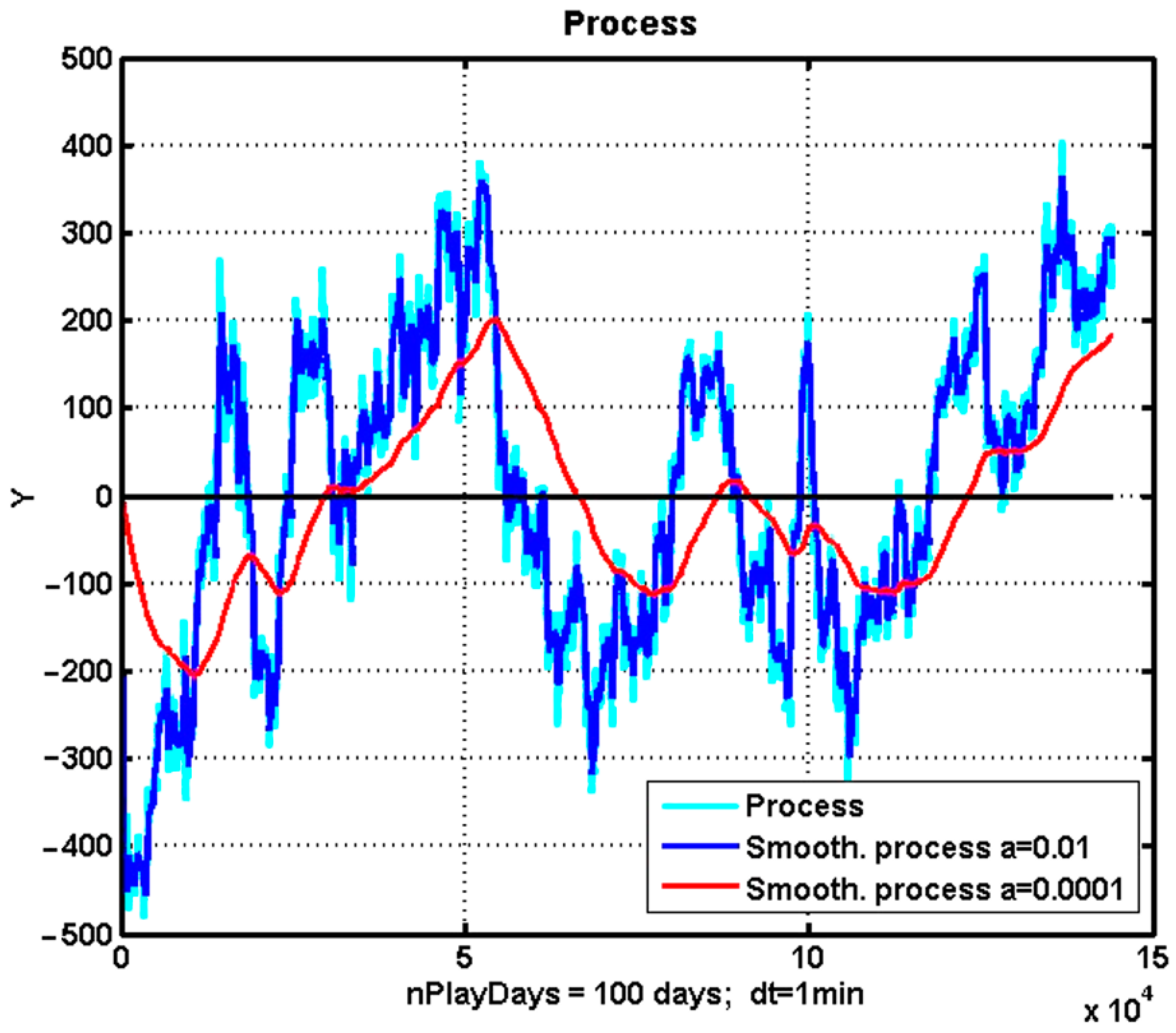
Figure 1. The process of changing the quotation of the EURUSD currency instrument and the results of its smoothing by an exponential filter over an observation interval of 100 days.
Jrfm 18 00033 g001
Figure 2. An example of the implementation of the TS01 trend strategy on a 10-day observation interval. The price changes observation series is shown as a sapphire line, with the smoothed values represented by a blue line. Position openings are marked by triangles (upward—blue, downward—red), and position closings are indicated by crosses.
Jrfm 18 00033 g002
Figure 3. The effectiveness of the TS01 trend strategy implementation example shown in Figure 2.
Jrfm 18 00033 g003
Figure 4. An example of the implementation of the TS01 trend strategy optimization on a 10-day observation interval. Position openings are marked by triangles (upward—blue, downward—red), and position closings are indicated by crosses.
Jrfm 18 00033 g004
Figure 5. Linear trends in the observation area. The downward trend is represented by a red line, while the upward trend is shown in pink.
Jrfm 18 00033 g005
Figure 6. An example of the implementation of the TS02 trend strategy on a 5-day observation interval. Position openings are marked by triangles (upward—blue, downward—red), and position closings are indicated by crosses.
Jrfm 18 00033 g006
Figure 7. An example of the implementation of the TS02 strategy with optimal parameters. Position openings are marked by triangles (upward—blue, downward—red), and position closings are indicated by rhombs.
Jrfm 18 00033 g007
Figure 8. An example of the implementation of the TS03 trend strategy on a 5-day observation interval. Position openings are marked by triangles, and position closings are indicated by circles.
Jrfm 18 00033 g008
Figure 9. An example of the implementation of the TS03 trend strategy on a 5-day observation interval with optimized parameters. Position openings are marked by triangles, and position closings are indicated by circles.
Jrfm 18 00033 g009
Figure 10. Comparison of the filtration quality of exponential and bidirectional filters over a 5-day observation interval.
Jrfm 18 00033 g010
Figure 11. Comparison of the results of filtering exponential and bidirectional filters on an observation interval of 4 days with a limitation on the number of reverse smoothing counts by a sliding observation window of size L = 100 min.
Jrfm 18 00033 g011
Figure 12. Application of the TS01 control strategy on a 25-day observation interval using an exponential filter. Position openings are marked by triangles (upward—blue, downward—red), and position closings are indicated by crosses.
Jrfm 18 00033 g012
Figure 13. Application of the TS01 control strategy for a 25-day observation interval using a bidirectional exponential filter. Position openings are marked by triangles (upward—blue, downward—red), and position closings are indicated by crosses.
Jrfm 18 00033 g013
Figure 14. Illustration of the decision-making process by the first fundamental expert. Green line represents a predicted period for long positions (expected price increase). Pink line denotes a period for short positions (expected price decline).
Jrfm 18 00033 g014
Figure 15. An example of using MES technology with the TS01 management strategy on a 25-day site. Position openings are marked by triangles (upward—blue, downward—red), and position closings are indicated by crosses.
Jrfm 18 00033 g015
Table 1. Analysis of the stability of the effectiveness of trend strategies.
123
TS01 Management Strategy
P* ( 0.05 , 50 , 5 ) ( 0.025 , 30 , 20 ) ( 0.02 , 50 , 5 )
R−629−651−1723
TS02 Management Strategy
P* ( 0.03 , 20 , 20 , 3 ) ( 0.01 , 40 , 20 , 3 ) ( 0.025 , 10 , 20 , 3 )
R−36765414
TS03 Management Strategy
P* ( 0.01 , 60 , 8 , 4 , 1 ) ( 0.011 , 30 , 11 , 12 , 2 ) ( 0.008 , 40 , 5 , 8 , 1 )
R−491−819−1845
Table 2. Analysis of the stability of the effectiveness of the TS01 trend strategy with a bidirectional filter on testing time intervals. Here, P* represents the set of optimal parameters obtained through parametric optimization of the strategy; R* denotes the results of optimization; R t refers to the results of testing; P+ represents the frequency of successful market entries during the testing phase.
123
P* ( 0.02 , 0.01 , 100 , 50 ) ( 0.02 , 0.01 , 100 , 40 ) ( 0.02 , 0.01 , 100 , 10 )
R*399−1651054
R t −629−818−1351
P+0.490.470.45
Disclaimer/Publisher’s Note: The statements, opinions and data contained in all publications are solely those of the individual author(s) and contributor(s) and not of MDPI and/or the editor(s). MDPI and/or the editor(s) disclaim responsibility for any injury to people or property resulting from any ideas, methods, instructions or products referred to in the content.