The Nonsense of Bitcoin in Portfolio Analysis

Abstract

The paper demonstrates the nonsense of using Bitcoin in financial investments. By using mean-variance financial analysis, stochastic dominance, CVaR, and the Shapley value theory as analytical statistical models, I show how Bitcoin performs poorly by comparing it against other traded assets. The conclusion is reached by analyzing daily freely available market data for the period 2018–2023.

1. Introduction

The purpose of this paper is to inquire why Bitcoin, despite it not being a valid medium of exchange nor a reliable store of value, is considered a legitimate investment instrument to be included in a portfolio of financial assets. Bitcoin proponents see it at par with other financial instruments traded in organized and regulated markets. There are a large number of well-respected research academicians who regard Bitcoin as a valid financial instrument and would like to have it regulated. This is of course a blasphemy for Bitcoin purists who claim that its main attraction is in its lack of regulation. Some professional analysts claim that Bitcoin should be recognized as a valid medium of exchange in order to allow it to legally register real-estate transactions. Renowned economists have been disparaged in the media when they point out the nonsense of using Bitcoin both as an investment and as a medium of exchange.

By reading some of the social networks, we observe that investors have not been deterred by the large number of financial scandals and scams involved in Bitcoin and other cryptocurrencies. It is not the purpose of the present paper to address this issue here. It is remarkable that serious investors and important investment bankers have diverted effort, money, and manpower to generate short-term revenues and invest into cryptocurrency markets. I am not checking their profits and losses; so I may err by writing this paper. However, I believe the remarks on Bitcoin written by Krugman (2022) in the New York Times are well founded.

A well-known political analyst has assured me that terrorist organizations do not fund their activities with Bitcoin, since blockchain records all transactions. Like other traffickers, terrorists prefer the use of gold and fiat currency to facilitate their illicit transactions. However, following Foley et al. (2019), it appears that approximately one-quarter of Bitcoin users are involved in illegal activity. From the intense literature on Bitcoin and cryptocurrency, I cite a few papers that analyze Bitcoin in portfolios: Akhtaruzzaman et al. (2020) used Bitcoin to build commodity portfolios, Bakry et al. (2021) investigated the performance of Bitcoin in various portfolios, Eisl et al. (2015) analyzed Bitcoin in portfolios and used the conditional value-at-risk metric to assess Bitcoin usefulness in diversification, and Platanakis and Urquhart (2020) approved of the inclusion of Bitcoin in portfolios to benefit investors. An important reference is Huberman et al. (2021), who analyzed the Bitcoin payment system, although I am convinced that most Bitcoin transactions are for the purpose of hoarding value and not for the payment of goods and services.

In order to analyze the use of Bitcoin in financial investments, I consider three classical models that revolve around risk-averse investors defined as prefering to receive the investment mean return and avoid participating in the investment.1 The first model is the standard Markowitz (1952) portfolio theory conceived in the mean-variance space. The second model, derived from von Neuman–Morgenstern expected utility theory, utilizes second-degree stochastic dominance (SSD) to compare Bitcoin to other assets using an absolute Lorenz curve and cumulative value-at-risk (CVaR). The third approach applies the Shapley value from cooperative game theory to establish the most valuable investment in building an efficient frontier portfolio with Bitcoin.

2. Bitcoin and Portfolio Management

In this section, I compare the ex-post performance of Bitcoin against the alternative of holding a portfolio of the most valued shares traded on Wall Street. For the classic Markowitz (1952) mean-variance (MV) paradigm, I used 108 shares that are all the components of the S&P100 index from January 2018 to May 2023.2 Stock returns are daily stock market data provided freely by Yahoo Finance. For Bitcoin, the quotes were also downloaded from Yahoo Finance. The starting date for the analysis was dictated by the introduction of Bitcoin futures on the Chicago Mercantile Exchange in December 2017. Before the year 2018, it was difficult to short Bitcoin positions using derivative instruments. Equity and bonds markets are closed on the weekends and holidays, leading to around 250 quotes per year. However, since Bitcoin is being traded 24/7, its quotes for weekends and holidays are removed, amounting to a difference of 100 data points per year. This manipulation increases the volatility of Bitcoin and its mean return as the returns move from Friday closing to Monday open. Indeed, the Bitcoin mean return including the weekend data stands at 0.104% and its daily standard deviation at 3.77%, whereas the statistics for Bitcoin for the same period (January 2018 to May 2023) for a 5-day week are 0.148% for the mean return equals and 4.497% for its standard deviation.3 The 108 stocks statistics for the period are provided in the Appendix A. With the sample at hand, we observe that the Bitcoin daily return has the largest standard deviation but not the largest mean.

We developed the two-time period MV model with Bitcoin and 108 traded securities, where investors minimize the portfolio variance subject to a mean return. We constructed a portfolio frontier in the MV space with N risky assets whose returns $\mathbf{r}$ that are linearly independent. This ensures the non-singularity of the variance-covariance matrix of asset returns $\mathbf{\Sigma }$. We also assume that at least two risky assets have different means. We denote by $\mathit{\mu }$ the vector of asset mean returns and $\mathbf{w}$ as the vector of portfolio weights such that ${\sum }_{i=1}^N{w}_i=1$. We assume $\mathbf{w}⋚0$, hereby allowing for short sales. A frontier portfolio is obtained by minimizing the variance portfolio ${\displaystyle \frac{1}{2}}{\sigma }_p^2={\displaystyle \frac{1}{2}}{\mathbf{w}}^{\prime }\mathbf{\Sigma }\mathbf{w}$ subject to a required mean ${\mu }_p={\mathbf{w}}^{\prime }\mathit{\mu }$ and the portfolio constraint $1={\mathbf{w}}^{\prime }\mathbf{l}$, where $\mathbf{l}$ is an N-vector of ones. As shown by Huang and Litzenberger (1988), the solution is obtained by minimizing the Lagrangian that includes the two constraints and deriving the first-order conditions (FOCs) for a minimum, with the second-order conditions being satisfied by the non-singularity of $\mathbf{\Sigma }$.

For the ease of presentation, we define the quadratic forms: $A={\mathbf{l}}^{\prime }{\mathbf{\Sigma }}^{-1}\mathit{\mu }$, $B={\mathit{\mu }}^{\prime }{\mathbf{\Sigma }}^{-1}\mathit{\mu }$, $C={\mathbf{l}}^{\prime }{\mathbf{\Sigma }}^{-1}\mathbf{l}$, and $D=BC-A^2.$ The scalars B and C are positive, since the matrix $\mathbf{\Sigma }$ is positive-definite and so is its inverse. As shown by Huang and Litzenberger (1988), the scalar D is also positive. From the FOCs for a minimum variance, the optimal portfolio weights for a given mean ${\mu }_p$ are obtained as follows:

$${\mathbf{w}}_p^{*}={\displaystyle \frac{1}{D}}[B·{\mathbf{\Sigma }}^{-1}\mathbf{l}-A·{\mathbf{\Sigma }}^{-1}\mathit{\mu }]+{\displaystyle \frac{1}{D}}[C·{\mathbf{\Sigma }}^{-1}\mathit{\mu }-A·{\mathbf{\Sigma }}^{-1}\mathbf{l}]{\mu }_p.$$

(1)

The frontier portfolios delineate a hyperbola in the mean–standard deviation space leading to the portfolio variance formula for a given ${\mu }_p$:

$${\sigma }_p^2={\mathbf{w}}_p^{\prime }\mathbf{\Sigma }{\mathbf{w}}_p={\displaystyle \frac{C}{D}}{({\mu }_p-{\displaystyle \frac{A}{C}})}^2+{\displaystyle \frac{1}{C}}.$$

(2)

Equation (2) is the basic formula for computing the frontier of optimal MV portfolios that is drawn as a solid line in Figure 1. From the statistics shown in the Appendix A, we have plotted the securities in Figure 1. First, we observe clearly that three stocks (AMD, NVDA, TSLA) outperformed Bitcoin, having a smaller standard deviation and a higher mean return. Furthermore, the efficient frontier constructed based on the 108 stocks clearly dominated the performance statistics of Bitcoin (BTC) for the period 2018–2023. This concludes the first examination based on the simple mean-variance model.

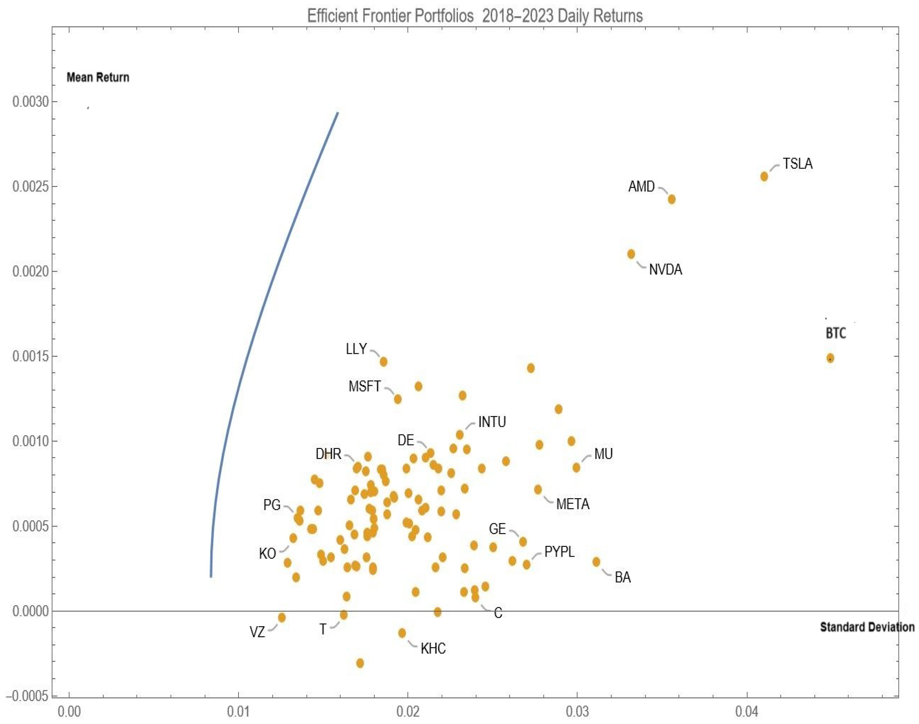
3. Bitcoin, the Lorenz, and CVaR

In this section5, the concepts of stochastic dominance are presented to demonstrate the unreasonableness of using Bitcoin in financial analysis. For that purpose, I use the absolute Lorenz curve as the main analytical tool to address second-degree stochastic dominance (SSD) and cumulative value-at-risk (CVaR) to value risky assets. Stochastic dominance theory developed by Hanoch and Levy (1969), Hadar and Russell (1969), and Rothschild and Stiglitz (1970) provides economic efficiency under expected utility maximization without specifying utility functions. This results in rules that compare cumulative probability distributions (CDFs) of asset returns.

Second-degree stochastic dominance (SSD), being mainly for risk-averse investors, is the most common model used in portfolio selection. By comparing the areas under the cumulative probabilities, SSD rules establish the necessary and sufficient conditions under which risky assets are preferred by all risk-averse expected utility maximizers. Computing the areas under the CDFs is not straightforward, as it must be done for all the probabilities. Then, the analyst is required to compare between the various areas. One more evident alternative was developed by Shorrocks (1983), who used the absolute Lorenz curve (named here the Lorenz) to establish SSD rules. The Lorenz expresses the cumulative return on the portfolio as a function of the cumulative probability distribution. Instead of comparing conditional areas under the CDFs, the following SSD rules are easier to visualize: For all risk-averse investors to prefer one asset over another, the Lorenz of one asset must lie entirely above the Lorenz of the other. In other words, asset A is preferred to asset B by all risk-averse investors if and only if

$$L_A\left(p\right)\ge L_B\left(p\right)\mathrm{for}0\le p\le 1,$$

(3)

where $L\left(p\right)$ is the Lorenz that, given the cumulative distribution $F\left(x\right)$ for asset x, is defined as

$$L\left(p\right)=\underset{-\infty }{\overset{x_p}{\int }}xf\left(x\right)dx\mathrm{for}-\infty \le x<\infty ;\mathrm{where}{x}_p\mathrm{is}\mathrm{given}\mathrm{by}p=\underset{-\infty }{\overset{x_p}{\int }}f\left(x\right)dx$$

(4)

where f is the asset density function. Gastwirth (1971) proposed an elegant simplified definition of the Lorenz curve by using the inverse of $F(x$) designated by $F^{-1}\left(t\right)=\underset{\mathit{x}}{\inf }\{x:F\left(x\right)\ge t\}$ which is written as

$$L\left(p\right)=\underset{0}{\overset{p}{\int }}{F}^{-1}\left(t\right)dtfor0\le t\le 1,$$

(5)

where p is the cumulative probability at which the return $x_p$ is obtained. In a sense, $x_p$ is the conditional mean return at cumulative probability p.

Let us explore the Lorenz drawn in Figure 2. Cumulative probabilities are shown on the horizontal axis; thus, returns are ranked in increasing value. The vertical axis reflects cumulative rates of returns weighted by the probabilities as formulated by Equation (3). Starting at (0,0), the Lorenz accumulates the sorted returns multiplied by their probabilities. Since the lowest returns can be losses, the Lorenz may result in negative values. The curve ends at the mean return $E\left(x\right)$ on the parallel vertical axis where all returns are used up and multiplied by their probabilities.

As explained by Shalit (2014), “…the rationale for using the Lorenz in financial analysis is rooted in the manner by which the Lorenz characterizes risk and mean return of investments for risk-averse investors. Such investors have concave utility functions that express declining marginal utility. The horizontal axis in Figure 2 shows the probabilities of asset returns ranked from those generating the lowest returns with the highest marginal utility to those generating the highest returns with the lowest marginal utility. The ranking of asset returns is the only information needed to sort an asset according to decreasing marginal utility. This ordering is specified by the cumulative returns multiplied by the probabilities of obtaining these returns. This is basically the Lorenz. The principle of distributing resources according to decreasing marginal utility or decreasing marginal product ensures that financial resources are allocated optimally. Using the Lorenz to manage portfolio risk guarantees that objective. Because the curve expresses asset behavior not as a function of returns over time but as the extent of having lower and higher returns, it provides much more relevant information about risk and return than periodical charts…”.

We now compare the Lorenz of Bitcoin against the Lorenz curves of the other securities to check whether it can be preferred by all risk-averse investors according to the stochastic dominance rules. The Lorenz curves of the 108 shares and Bitcoin were computed for the period 2018–2023. This is presented in Figure 3.

The results are convincing for the period at hand. Bitcoin was SSD-dominated by most 108 securities. Although in general, Bitcoin revealed a higher mean return, its risk as expressed by a series of larger negative returns produced a Lorenz that is well below most of the other securities. It is true that the Lorenz curves intersect at some point, so the the results are not overwhelming. Indeed, using the Lorenz to value SSD provides an incomplete ranking of assets. Hence, one can look at the necessary conditions for stochastic dominance that use the mean and Gini’s mean difference as statistics. Following Shalit and Yitzhaki (2010), we obtain from the Lorenz the two statistics that express risk and expected return. The latter is located at the terminal point of the Lorenz on the parallel vertical axis at $p=1$. The risk underlying the Lorenz is obtained by computing the vertical differences between the Lorenz and a virtual riskless asset with the same expected return as the asset labeled the line of safe asset (LSA). In Figure 2, the LSA is a straight line drawn from the origin (0, 0) to the mean (${\mu }_x$, 1). The LSA expresses the expected return ${\mu }_x$ multiplied by the probability p as plotted in Figure 2. The area between the LSA and the Lorenz is Gini’s mean difference (GMD). In portfolio management, it is convenient to use one half of GMD that we label here as the Gini:

$$GMD/2\equiv {\Gamma }_x=2cov[x,F\left(x\right)]$$

(6)

As seen in Figure 2 and explained above, the Gini is easily obtained by computing the area between the LSA and the Lorenz as follows:

$${\displaystyle \frac{1}{2}}\Gamma =\underset{0}{\overset{1}{\int }}[{\mu }_{x}p-L\left(p\right)]dp=cov[x,F\left(x\right)].$$

(7)

Now, we can address the necessary conditions for SSD derived from the Lorenz. The mean being the terminal point on the Lorenz is the first condition. A dominating asset should have a greater expected return, as expressed by Equation (8) The second condition, as expressed by Equation (9), looks at the area under the Lorenz that is the entire area below the LSA and the area above the Lorenz, which is the Gini. The other necessary condition for SSD is that the area below the Lorenz of the dominating asset be greater than the area below the Lorenz of the dominated asset. This area is one-half the mean return subtracted by the Gini. We can call this area the Gini adjusted mean return. These requirements explain the necessary conditions for SSD first enunciated by Yitzhaki (1982) as the mean Gini (MG) necessary conditions

$${\mu }_x\ge {\mu }_y$$

(8)

$${\mu }_x-{\Gamma }_x\ge {\mu }_y-{\Gamma }_y$$

(9)

for asset x to the SSD dominate asset y. To assert dominance, I use these conditions to rank the shares and Bitcoin as they appear in

Table 1. Bitcoin and stocks ranked according to Gini-adjusted mean return.

Symbol	Mean	Gini	$\mathit{\mu }-\mathbf{\Gamma }$	Symbol	Mean	Gini	$\mathit{\mu }-\mathbf{\Gamma }$	Symbol	Mean	Gini	$\mathit{\mu }-\mathbf{\Gamma }$
PEP	0.05%	0.65%	−0.60%	ACN	0.07%	0.91%	−0.84%	CAT	0.06%	1.11%	−1.05%
PG	0.05%	0.67%	−0.61%	MO	0.01%	0.85%	−0.84%	ADI	0.08%	1.14%	−1.06%
KO	0.04%	0.66%	−0.62%	CB	0.04%	0.88%	−0.84%	AXP	0.07%	1.13%	−1.06%
MDLZ	0.06%	0.68%	−0.62%	V	0.07%	0.92%	−0.85%	AVGO	0.13%	1.19%	−1.07%
JNJ	0.03%	0.65%	−0.62%	SPGI	0.08%	0.93%	−0.85%	PNC	0.03%	1.10%	−1.07%
MCD	0.06%	0.69%	−0.63%	TMO	0.09%	0.94%	−0.85%	USB	0.00%	1.08%	−1.08%
WMT	0.05%	0.70%	−0.65%	CSCO	0.05%	0.91%	−0.86%	BAC	0.03%	1.11%	−1.08%
CL	0.02%	0.68%	−0.66%	UNP	0.05%	0.92%	−0.87%	ISRG	0.09%	1.18%	−1.08%
VZ	0.00%	0.65%	−0.66%	PLD	0.08%	0.95%	−0.88%	INTU	0.10%	1.22%	−1.11%
MMC	0.07%	0.74%	−0.67%	AMT	0.05%	0.92%	−0.88%	AMZN	0.08%	1.20%	−1.11%
MRK	0.08%	0.75%	−0.67%	SBUX	0.07%	0.95%	−0.88%	ADBE	0.09%	1.21%	−1.12%
BRK-B	0.05%	0.72%	−0.67%	CCI	0.03%	0.91%	−0.88%	BKNG	0.06%	1.18%	−1.12%
COST	0.09%	0.77%	−0.68%	CSX	0.06%	0.95%	−0.89%	FDX	0.02%	1.17%	−1.14%
DUK	0.03%	0.73%	−0.70%	MSFT	0.12%	1.01%	−0.89%	CRM	0.08%	1.25%	−1.17%
BMY	0.03%	0.78%	−0.75%	UPS	0.06%	0.95%	−0.89%	C	0.01%	1.18%	−1.17%
LMT	0.05%	0.82%	−0.77%	SYK	0.07%	0.96%	−0.90%	WFC	0.01%	1.19%	−1.18%
NEE	0.07%	0.84%	−0.77%	CVS	0.03%	0.93%	−0.90%	AIG	0.04%	1.24%	−1.20%
BDX	0.03%	0.81%	−0.78%	CMCSA	0.02%	0.93%	−0.91%	INTC	0.01%	1.21%	−1.20%
AMGN	0.04%	0.82%	−0.78%	MMM	−0.03%	0.88%	−0.91%	SCHW	0.04%	1.24%	−1.20%
LLY	0.15%	0.92%	−0.78%	KHC	−0.01%	0.91%	−0.92%	TFC	0.01%	1.22%	−1.21%
ABT	0.06%	0.86%	−0.80%	JPM	0.05%	0.99%	−0.94%	QCOM	0.09%	1.33%	−1.24%
HON	0.04%	0.85%	−0.80%	RTX	0.04%	0.99%	−0.95%	META	0.07%	1.35%	−1.28%
ADP	0.07%	0.87%	−0.80%	LOW	0.09%	1.04%	−0.95%	COP	0.10%	1.40%	−1.31%
LIN	0.08%	0.89%	−0.81%	TGT	30.09%	1.03%	−0.95%	NOW	0.14%	1.46%	−1.32%
CME	0.05%	0.86%	−0.81%	AAPL	0.13%	1.08%	−0.95%	GM	0.03%	1.37%	−1.34%
MDT	0.03%	0.84%	−0.81%	MA	0.09%	1.04%	−0.95%	GE	0.04%	1.41%	−1.37%
DHR	0.08%	0.90%	−0.81%	GOOGL	0.08%	1.05%	−0.97%	PYPL	0.03%	1.40%	−1.37%
PFE	0.04%	0.85%	−0.81%	BLK	0.05%	1.03%	−0.98%	NFLX	0.10%	1.51%	−1.41%
T	0.00%	0.81%	−0.81%	NKE	0.07%	1.05%	−0.98%	AMAT	0.12%	1.56%	−1.44%
ORCL	0.08%	0.90%	−0.81%	GS	0.05%	1.04%	−1.00%	BA	0.03%	1.52%	−1.49%
IBM	0.03%	0.84%	−0.82%	TXN	0.07%	1.07%	−1.00%	MU	0.08%	1.63%	−1.54%
PM	0.03%	0.85%	−0.82%	CVX	0.06%w	1.06%	−1.01%	NVDA	0.21%	1.77%	−1.56%
ZTS	0.08%	0.90%	−0.82%	DIS	0.01%	1.03%	−1.02%	AMD	0.24%	1.90%	−1.66%
ABBV	0.06%	0.89%	−0.83%	CI	0.04%	1.07%	−1.03%	TSLA	0.26%	2.16%	−1.91%
HD	0.06%	0.89%	−0.83%	DE	0.09%	1.12%	−1.03%	BTC	0.15%	2.30%	−2.16%
UNH	0.08%	0.91%	−0.83%	MS	0.07%	1.12%	−1.04%
TMUS	0.07%	0.91%	−0.84%	XOM	0.06%	1.11%	−1.05%

The mean return minus the Gini expresses the necessary condition of Equation (9) for second-degree stochastic dominance. The ranking shows what assets are most preferred by risk-averse investors.

. The ranking with respect to the mean and the Gini-adjusted mean return show without any doubt the inferiority of Bitcoin according to SSD rule expressed by Equation (9). Actually, to visualize the MG necessary conditions for SSD, one shoud delineate the results of Table 1 in a mean vs Gini-adjusted mean return space. Here, I use only condition (9). Although it has a larger mean, Bitcoin is mean Gini dominated by all other assets.

Related to the Lorenz, there is an additional criterion that we like to use that is the value-at-risk (VaR). The measure quantifies exposure to risk as the amount needed to keep in a safe asset to overcome the default. VaR is a safety-first risk measure defined as the negative quantile of probability p expressed as

$$VaR\left(p\right)=-F^{-1}\left(p\right)$$

(10)

As we can observe from Equation (10), $VaR\left(p\right)$ is only one point on the Lorenz obtained directly from the cumulative distribution function. However, it is well established that VaR lacks the basic properties of a valid risk measure, as explained by Artzner et al. (1999). For coping with VaR‘s lack of coherence, the conditional value-at-risk (CVaR) was developed by Rockafellar and Uryasev (2000). The basic idea is to calculate $CVaR\left(p\right)$ as the mean value of all the quantiles below the original VaR in the lower tail of the cumulative distribution function. This can basically be obtained directly from the Lorenz:

$$CVaR\left(p\right)=-{\displaystyle \frac{1}{p}}\underset{0}{\overset{p}{\int }}{F}^{-1}\left(t\right)dt=-{\displaystyle \frac{L\left(p\right)}{p}}$$

(11)

In Figure 2, the $CVaR\left(\alpha \right)$ for probability $\alpha$ is the slope of the straight line that runs from (0,0) to $(\alpha ,L(\alpha )$). Under these circumstances, the estimated CVaR becomes a specific value of the Lorenz. Hence, for a given data set, the CVaR is estimated by ranking and summing up the observations. The CVaR at 5% and at 10% for our securities and Bitcoin are presented in

Table 2. CVaR (5%) and CVaR(10%) for all assets.

Symbol	CVaR5%	CVaR10%	Symbol	CVaR5%	CVaR10%	Symbol	CVaR5%	CVaR10%
BTC	28.73%	14.30%	CVX	13.59%	6.76%	NFLX	19.31%	9.61%
AAPL	13.31%	6.62%	DE	14.18%	7.05%	NKE	13.35%	6.65%
ABBV	11.38%	5.66%	DHR	11.28%	5.61%	NOW	18.39%	9.14%
ABT	11.03%	5.48%	DIS	13.54%	6.74%	NVDA	21.94%	10.90%
ACN	11.42%	5.68%	DUK	9.38%	4.67%	ORCL	11.11%	5.53%
ADBE	15.35%	7.64%	FDX	15.40%	7.66%	PEP	8.05%	4.01%
ADI	14.62%	7.27%	GE	18.59%	9.25%	PFE	11.06%	5.50%
ADP	11.01%	5.48%	GM	18.03%	8.97%	PG	8.42%	4.19%
AIG	15.98%	7.95%	GOOGL	13.29%	6.62%	PLD	12.07%	6.01%
AMAT	20.07%	9.98%	GS	13.61%	6.77%	PM	11.11%	5.53%
AMD	23.32%	11.61%	HD	11.35%	5.65%	PNC	14.33%	7.13%
AMGN	10.55%	5.25%	HON	10.91%	5.43%	PYPL	18.56%	9.23%
AMT	12.00%	5.97%	IBM	10.95%	5.45%	QCOM	16.93%	8.42%
AMZN	15.26%	7.60%	INTC	16.17%	8.05%	RTX	12.55%	6.25%
AVGO	14.90%	7.41%	INTU	15.39%	7.66%	SBUX	11.85%	5.90%
AXP	14.20%	7.06%	ISRG	14.84%	7.38%	SCHW	16.41%	8.16%
BA	19.70%	9.81%	JNJ	8.35%	4.16%	SPGI	11.74%	5.84%
BAC	14.50%	7.21%	JPM	12.74%	6.34%	SYK	12.17%	6.05%
BDX	10.64%	5.29%	KHC	12.16%	6.05%	T	10.82%	5.38%
BKNG	15.29%	7.61%	KO	8.36%	4.16%	TFC	16.06%	7.99%
BLK	13.25%	6.60%	LIN	11.26%	5.60%	TGT	12.89%	6.41%
BMY	10.18%	5.06%	LLY	10.97%	5.46%	TMO	11.99%	5.95%
BRK-B	9.21%	4.58%	LMT	10.31%	5.13%	TMUS	11.44%	5.69%
C	15.60%	7.76%	LOW	13.01%	6.47%	TSLA	26.35%	13.11%
CAT	14.41%	7.17%	MA	13.07%	6.50%	TXN	13.93%	6.93%
CB	11.32%	5.63%	MCD	8.59%	4.27%	UNH	11.36%	5.65%
CCI	11.98%	5.96%	MDLZ	8.46%	4.21%	UNP	11.89%	5.91%
CI	13.98%	6.95%	MDT	10.97%	5.46%	UPS	12.13%	6.03%
CL	8.92%	4.43%	META	17.34%	8.63%	USB	14.14%	7.04%
CMCSA	12.41%	6.18%	MMC	9.21%	4.58%	V	11.56%	5.75%
CME	11.00%	5.47%	MMM	12.08%	6.02%	VZ	8.74%	4.35%
COP	17.96%	8.93%	MO	11.33%	5.64%	WFC	15.63%	7.78%
COST	9.50%	4.72%	MRK	9.28%	4.62%	WMT	8.89%	4.42%
CRM	16.04%	7.98%	MS	14.37%	7.15%	XOM	14.41%	7.16%
CSCO	11.70%	5.82%	MSFT	12.41%	6.18%	ZTS	11.46%	5.70%
CSX	12.18%	6.06%	MU	21.43%	10.66%
CVS	12.40%	6.17%	NEE	10.52%	5.23%

The CVaR values are computed using $-L\left(\alpha \right)/\alpha$ for $\alpha$ at 5% and 10%. Assets are ranked alphabeticaly by their symbols.

.

The larger CVaR, the riskier the stock. From Table 2, we see that BTC ranks among the riskier ones. No surprise here. This is particularly true for the stocks NVDA, AMD, and TSLA vs Bitcoin. The main difference is that the CVaR considers only low-return risks for a given probability, whereas the Lorenz and the mean Gini conditions for SSD consider the risk and mean return for the entire distribution. Using the CVaR is only the first element to rank downside risk; the next step involves using the Lorenz and the mean Gini conditions to obtain a complete picture of risk and return and compare Bitcoin to portfolio assets.

4. The Shapley Value of Bitcoin in a Efficient Portfolio

In order to compute the exact value of Bitcoin in a standard investment model, I am using the Shapley value from cooperative game theory. I consider a portfolio of stocks as an n-person cooperative game where the financial assets are players in the game. The goal is to measure the contribution of each stock to the general outcome of the portfolio. The Shapley value extracts the true and exact contribution of each stock to the portfolio’s total value. The presentation of this section follows Shalit (2021).

The game purpose is to minimize portfolio risk expressed by the variance for a given mean return. For a set N of n securities, the Shapley value is calculated from the contribution of each and every security in the portfolio. To capture the way each security contributes to the entire portfolio, we compute the risk v for each and every subset of stocks $S\subset N$. In total, we have $2^N$ portfolios or coalitions, including the empty set. The marginal contribution of each security k to the subset portfolio S is given by $v\left(S\right)-v(S\backslash \left\{k\right\})$, where $v\left(S\right)$ is the risk of portfolio S, and $v(S\backslash \{k\left\}\right)$ is the risk of the portfolio S without security k. Portfolios are predefined, and all the orderings are equally probable. Hence, $S\backslash \left\{k\right\}$ is the portfolio that precedes k, and its contribution to coalition S is computed when all the orderings of S are accounted for. Given equally probable orderings, we compute their expected marginal contribution. Therefore, we need the probability that, for a given ordering, the subset $S\subset N,k\subset S$ is seen as the union of security k and all the securities that precede it. Two probabilities are used here: First, the probability that k is in s (s being the number of stocks in S) being equal to $1/n$, and second, that $S\backslash \left\{k\right\}$ arises when $s-1$ securities are randomly chosen from $N\backslash \left\{k\right\}$, that is, $(n-s)!(s-1)!/(n-1)!$.

The Shapley value for security k is obtained by averaging the marginal contributions to the risk of all portfolios for the set of N securities and the risk function v, which in mathematical terms is written as

$$S{h}_k(N,v)={\displaystyle \sum _{S\subset N,k\subset S}}{\displaystyle \frac{(n-s)!(s-1)!}{n!}}[v\left(S\right)-v(S\backslash \left\{k\right\})]$$

(12)

or, alternatively,

$$S{h}_k(N,v)=\sum _{S\subset N,k\subset S}{\displaystyle \frac{s!(n-s-1)!}{n!}}[v(S\cup \left\{k\right\})-v\left(S\right)].$$

(13)

Shapley value theory works best with a single attribute imputed to all game participants; thus, I used optimal portfolios whose expected returns are always at their minimum risk. Consider the set of frontier portfolios generated by minimizing the portfolio variance for a given expected return. The portfolio frontier in the mean–standard deviation space was elaborated in Section 2 above. The result is the variance formulated by Equation (2) that is the set of the optimal MV portfolios. That variance is used to calculate the Shapley value of assets on the MV efficient frontier. For the mean return ${\mu }_p,$ the variance of Equation (2) can be written equivalently as

$${\sigma }_p^2={\displaystyle \frac{1}{D}}(C{\mu }_p^2-2A{\mu }_p+B).$$

(14)

Then, for an arbitrary set of required mean returns ${\mu }_p$, we calculate with Equation (14) the frontier portfolio variance for each subset $S\cup i\subseteq N$. The Shapley value is computed following Equation (13) using the variance-covariance matrix ${\mathbf{\Sigma }}_S$ and the quadratic forms $A_S={\mathbf{l}}_S^{\prime }{\mathbf{\Sigma }}_S^{-1}{\mathit{\mu }}_S$, $B_S={\mathit{\mu }}_S^{\prime }{\mathbf{\Sigma }}_S^{-1}{\mathit{\mu }}_S$, $C_S={\mathbf{l}}_S^{\prime }{\mathbf{\Sigma }}_S^{-1}{\mathbf{l}}_S$, and $D_S=B_S{C}_S-A_S^2$ for all the $2^N$ subsets $S\subseteq N$. The Shapley value for each stock i in an optimal frontier portfolio subject to a given mean ${\mu }_p$ is obtained as

$$S{h}_i({\sigma }_p^2;{\mu }_p)=\sum _{s=0}^{N-1}\sum _{S\subset N\backslash i}{\displaystyle \frac{(n-s-1)!s!}{n!}}[{\sigma }_p^2({\mu }_p,S\cup \left\{i\right\})-{\sigma }_p^2({\mu }_p,S)]\forall i\in N.$$

(15)

Finally, for a given return ${\mu }_p$, the Shapley values add up to their optimal portfolio variance at ${\mu }_p$ as

$$\sum _{i=1}^{N}S{h}_i({\sigma }_p^2;{\mu }_p)={\sigma }_p^2\left({\mu }_p\right).$$

(16)

It now seems natural to discuss the Shapley value as expressed by Equation (15) for an asset in an optimal portfolio. Given that efficient portfolios have the lowest variance for a given mean, the incremental risks ${\sigma }_p^2({\mu }_p,S\cup \left\{i\right\})-{\sigma }_p^2({\mu }_p,S)$ are non-positive for any asset i and any set S that does not contain i. Indeed, as assets are added to the portfolio, the variance does not increase. However, Shapley value computation also includes the incremental risk of going from an empty portfolio to a portfolio of one risky asset i whose increment is usually positive. Hence, as it is shown in the empirical analysis, Shapley values of assets in optimal portfolios can be either negative or positive. Negative Shapley values imply that these assets reduce their risk contribution to the portfolio as the mean return increases. Positive Shapley values imply increasing risk assets along the efficient frontier and therefore increase mean return.

For the empirical analysis, I have reduced the number of assets because of the dimensionality of calculating the Shapley value. I am confident that in the short future, quantum computing will solve the dimensionality issue and calculate Shapley value for any portfolio size. Many other techniques are available to calculate the exact contribution of individual stocks to their portfolio, but the many attempts made with the Shapley values are the most practical given the present tools. In the present research, I have chosen 12 assets that include Bitcoin, the major stock market indices, and single stocks to have a complete picture of the stock market to compare with Bitcoin. The statistics for these assets are reported in Appendix A.

The Shapley value results are presented below on

Table 3. Shapley values of assets on the efficient frontier.

Symbol	Mean	Shapley Value
AAPL	0.132%	0.113%
BTC	0.149%	0.363%
EEM	0.006%	0.007%
GLD	0.032%	−0.259%
IXIC	0.060%	0.034%
IYE	0.046%	0.126%
JNK	0.010%	−0.479%
NVDA	0.210%	0.231%
QQQ	0.076%	0.040%
SPY	0.050%	−0.053%
TSLA	0.255%	0.326%
XLK	0.090%	0.053%

and plotted in Figure 4 in the mean return–Shapley value graph. In a sense, we compare the asset mean return against the risk expressed by their optimal contribution to the portfolio. What we confirmed by using the Shapley value in an efficient portfolio of major financial assets and BTC is that Bitcoin is not the most valued financial instrument in terms of risk and mean return.

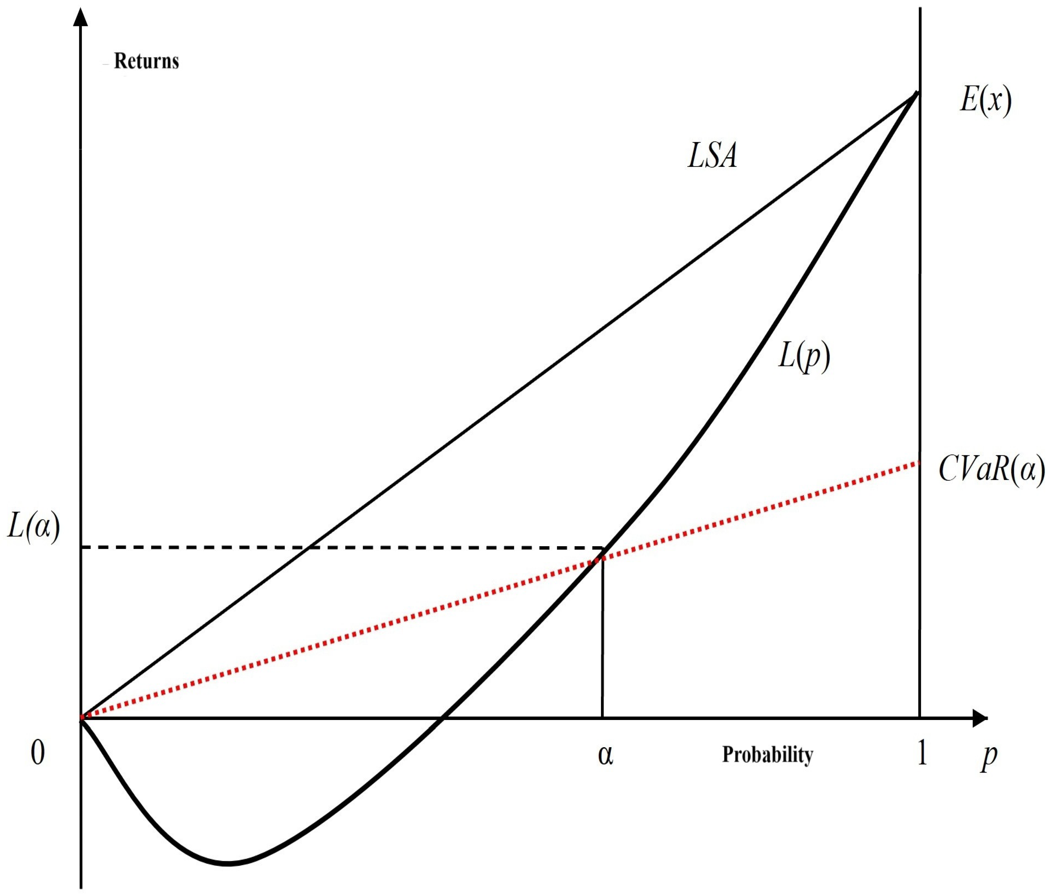
5. Conclusions and Implications

Daily financial market data from the period 2018–2023 were used in three different standard rational models to confirm statistically that Bitcoin is an overpriced asset that does not deserve to be included in a financial portfolio. Mean-variance analysis, second-degree stochastic dominance, and Shapley values affirm this result to a certain extent. This is true for all risk-averse investors. Furthermore, because Bitcoin is an unregulated asset traded on days and hours when investors are enjoying their weekends, its movements cannot be used efficiently with other financial assets. For institutions and individuals who construct portfolios using stock market assets for pensions and retirement accounts, including Bitcoin would be tantamount of using other risky instruments such as casinos, sport betting, and state lotteries in the portfolio. To include Bitcoin in financial portfolios and avoid weekend trading, one would need to use its many derivative instruments that can protect its volatility and include the few Bitcoin ETFs that are traded like regular shares.

References

1. Akhtaruzzaman, M., Sensoyc, A., & Corbet, S. (2020). The influence of Bitcoin on portfolio diversification and design. Finance Research Letters, 37, 101344. [Google Scholar] [CrossRef]
2. Artzner, P., Delbaen, F., Eber, J.-M., & Heath, D. (1999). Coherent measures of risk. Mathematical Finance, 9, 203–228. [Google Scholar] [CrossRef]
3. Bakry, W., Rashid, A., Al-Mohamad, S., & El-Kanj, N. (2021). Bitcoin and porfolio diversification: A portfolio optimization approach. Journal of Risk and Financial Management, 14, 282. [Google Scholar] [CrossRef]
4. Eisl, A., Gasser, S. M., & Weinmayer, K. (2015). Caveat emptor: Does bitcoin improve portfolio diversification? SSRN, 2408997. [Google Scholar] [CrossRef]
5. Engle, R., & Rangel, J. (2009). The Factor-Spline-GARCH model for high and low frequency correlations. Working Papers, No. 2009-03. Banco de México, Ciudad de México. [Google Scholar]
6. Foley, S., Karlsen, J. R., & Putnins, T. J. (2019). Sex, drugs, and bitcoin: How much illegal activity is financed through cryptocurrencies? The Review of Financial Studies, 32(5), 1798–1853. [Google Scholar] [CrossRef]
7. Gastwirth, J. L. (1971). A general definition of the lorenz curve. Econometrica, 39, 1037–1039. [Google Scholar] [CrossRef]
8. Hadar, J., & Russell, W. R. (1969). Rules for ordering uncertain prospects? American Economic Review, 59, 25–34. [Google Scholar]
9. Hanoch, G., & Levy, H. (1969). The efficiency analysis of choice involving risk. Review of Economic Studies, 36, 335–346. [Google Scholar] [CrossRef]
10. Huang, C.-F., & Litzenberger, R. H. (1988). Foundations for financial economics. Elsevier Science Publishing Co. [Google Scholar]
11. Huberman, G., Leshno, J. D., & Moallemi, C. (2021). Monopoly without a monopolist: An economic analysis of the Bitcoin payment system. Review of Economic Studies, 88(6), 3011–3040. [Google Scholar] [CrossRef]
12. Krugman, P. (2022, November 18). Is this the end game for crypto? New York Times, 15. [Google Scholar]
13. Markowitz, H. (1952). Portfolio selection. Journal of Finance, 7(1), 77–91. [Google Scholar]
14. Platanakis, E., & Urquhart, A. (2020). Should investors include bitcoin in their portfolios? A portfolio theory approach. The British Accounting Review, 52(4), 100837. [Google Scholar] [CrossRef]
15. Rockafellar, R., & Uryasev, S. (2000). Optimization of conditional value-at-risk. Journal of Risk, 2, 21–41. [Google Scholar] [CrossRef]
16. Rothschild, M., & Stiglitz, J. (1970). Increasing risk i: A definition. Journal of Economic Theory, 2, 66–84. [Google Scholar] [CrossRef]
17. Shalit, H. (2014). Portfolio risk management using the Lorenz curve. Journal of Portfolio Management, 40(3), 152–159. [Google Scholar]
18. Shalit, H. (2021). The Shapley value decomposition of optimal portfolios. Annals of Finance, 17(1), 1. [Google Scholar] [CrossRef]
19. Shalit, H., & Yitzhaki, S. (2010). How does beta explain stochastic dominance efficiency? Review of Quantitative Finance and Accounting, 35(4), 431–444. [Google Scholar] [CrossRef]
20. Shorrocks, A. F. (1983). Ranking income distributions. Economica, 50, 3–17. [Google Scholar] [CrossRef]
21. Yitzhaki, S. (1982). Stochastic dominance, mean variance, and Gini’s mean difference. American Economic Review, 72(1), 178–185. [Google Scholar]
Figure 1. Efficient frontier, stocks, and Bitcoin.4
Jrfm 18 00125 g001
Figure 2. The Lorenz curve.6
Jrfm 18 00125 g002
Figure 3. Lorenz curves of all assets for 2018–2023 daily returns.
Jrfm 18 00125 g003
Figure 4. Shapley values vs means of frontier portfolio assets for 2018–2013 daily returns.
Jrfm 18 00125 g004