Abstract
Against the backdrop of the “dual circulation” development pattern and the in-depth advancement of the Regional Comprehensive Economic Partnership (RCEP), the interconnection between China and global financial markets has significantly intensified. The spatio-temporal correlation risks faced in cross-border investment activities have become highly complex, posing a severe challenge to traditional investment risk prediction methods. Existing research has three limitations: first, traditional analytical tools struggle to capture the dynamic spatio-temporal correlations among financial markets; second, mainstream deep learning models lack the ability to directly output interpretable economic parameters; third, the uncertainty of model prediction results has not been systematically quantified for a long time, leading to a lack of credibility assessment in practical applications. To address these issues, this study constructs a spatio-temporal graph convolutional neural network panel regression model (STGCN-PDR) that incorporates uncertainty quantification. This model innovatively designs a hybrid architecture of “one layer of spatial graph convolution + two layers of temporal convolution”, modeling the spatial dependencies among global stock markets through graph networks and capturing the dynamic evolution patterns of market fluctuations with temporal convolutional networks. It particularly embeds an interpretable regression layer, enabling the model to directly output regression coefficients with economic significance, significantly enhancing the decision-making reference value of risk prediction. By designing multi-round random initialization perturbation experiments and introducing the coefficient of variation index to quantify the stability of model parameters, it achieves a systematic assessment of prediction uncertainty. Empirical results based on stock index data from 20 countries show that compared with the benchmark models, STGCN-PDR demonstrates significant advantages in both spatio-temporal feature extraction efficiency and risk prediction accuracy, providing a more interpretable and reliable quantitative analysis tool for cross-border investment decisions in complex market environments.
1. Introduction
In the context of China’s “dual circulation” development strategy and the deepening implementation of the Regional Comprehensive Economic Partnership (RCEP), the integration between China and global financial markets has become increasingly pronounced (Peng & Li, 2010). According to statistical data, cross-border direct investment reached USD 2.3 trillion in 2024, representing a 47% increase compared to before the RCEP took effect (Sergio & Wedemeier, 2025). The active cross-border investment activities have significantly strengthened the spatial correlations among global financial markets. Specifically, the average daily return correlation among different financial markets and products increased by 22% compared to 2019, while the time lag for risk transmission ranges from 48 h to 5 trading days. These characteristics indicate that investment risks exhibit complex spatio-temporal correlation patterns (Peng & Li, 2010). Furthermore, sustainable development initiatives, such as cross-border e-commerce pilot zones, have been shown to significantly boost regional economic growth (L. F. Yang et al., 2023), further intensifying these interconnections and the associated risks. This “dynamic spatial correlation and multi-scale temporal dependence” risk structure poses unprecedented challenges to the analysis and prediction of international investment risks. Consequently, effectively capturing and utilizing spatio-temporal correlations to enhance the accuracy of risk prediction has become an urgent issue in financial risk management.
Traditional financial time series analysis methods are predominantly based on linear and stationary assumptions (Box, 2013). Box–Jenkins time series models, such as autoregressive (AR) and ARIMA models, were widely applied in financial risk prediction. However, these models focus solely on the time series changes within a single market and fail to account for potential spatial dependencies among different regions or markets (Box, 2013). Subsequent developments in nonlinear time series methods, such as ARCH and GARCH models, relaxed the linear assumption and better captured the clustering of market volatility. Nevertheless, they still exhibit limitations in addressing the spatial correlation of risks (Engle, 1982; Bollerslev, 1986).
Current spatio-temporal modeling approaches can be categorized into two main types: statistical methods and artificial intelligence methods. Classic spatio-temporal statistical models, including ST-ARIMA (Martin & Oeppen, 1975), ST-Kriging (Dimitrakopoulos & Luo, 1994), and Bayesian Maximum Entropy (BME) (Skilling, 2013), provide explanations for spatio-temporal correlations from a statistical perspective but encounter limitations in model construction (Xu et al., 2021). First, these models establish time series models independently for each spatial location, ignoring intrinsic connections among different locations. Second, they construct overall spatial models at each time slice, making it challenging to capture dynamic changes in the time dimension. Moreover, their fixed structures render them incapable of handling the complex nonlinear and non-stationary features inherent in financial data (Reichstein et al., 2019).
Machine learning and deep learning, as data-driven tools, have demonstrated superior performance in various domains, such as weather forecasting and traffic flow prediction (Akbari Asanjan et al., 2018; Chen et al., 2017). Recent applications in finance show promise, such as the EOAEFA neural network for time series forecasting (Nayak et al., 2024) and hybrid deep learning–GAN models for VaR and ES estimation (Wang et al., 2024). Machine learning algorithms, such as Support Vector Machines (SVMs) (Cortes & Vapnik, 1995) and Random Forests (RFs) (Breiman, 2001), can handle certain nonlinear relationships but face limitations in terms of modeling capabilities and computational efficiency when dealing with large-scale spatio-temporal data scenarios. Deep learning, leveraging deep neural networks, excels at automatically extracting high-dimensional nonlinear features. For instance, Convolutional Neural Networks (CNNs) are adept at capturing spatial patterns, while Long Short-Term Memory (LSTM) networks are suitable for time series modeling (Tran et al., 2018; Shi et al., 2015; Lu et al., 2019). However, the complexity and limited sample size of financial data lead to unstable application effects of these models. More critically, deep learning models are often regarded as “black boxes”, making it difficult to output regression coefficients with clear spatio-temporal economic meanings or to intuitively assess the influence of individual factors on risks (Chen et al., 2017). Additionally, existing deep learning-based risk prediction studies generally overlook the quantification of model prediction uncertainty, providing only point predictions without evaluating prediction confidence intervals. This limitation poses significant risks in high-stakes financial decision-making. For example, early studies in online medical recommendation systems failed to consider prediction uncertainty, which is now recognized as a critical research gap (Cui et al., 2025). Similarly, environmental regulations have been shown to influence the technological complexity of exports (W. X. Yang et al., 2024), introducing an additional layer of macroeconomic uncertainty that warrants integration into modeling endeavors. By the same token, the field of financial risk prediction urgently requires addressing this issue.
To address the aforementioned challenges and research gaps, this paper proposes a Spatio-Temporal Graph Convolutional Regression Model (STGCN-PDR) that integrates uncertainty quantification. This model combines the spatio-temporal feature extraction capabilities of deep learning with the interpretability of regression analysis, aiming to extract spatio-temporal features from financial data and directly output interpretable spatio-temporal correlation regression coefficients. Through a panel regression structure and statistical loss function, it provides a foundation for systematic uncertainty analysis in risk prediction. The primary contributions of this paper are summarized as follows:
(1) Innovative Spatio-Temporal Risk Prediction Framework: The spatio-temporal graph convolutional neural network is applied to international investment risk prediction, constructing a novel model tailored for stock index panel data. This innovation offers new ideas and tools for analyzing financial spatio-temporal data and achieves simultaneous capture of spatial correlations and temporal dynamics in cross-border markets.
(2) Enhanced Model Interpretability: Building upon the existing STGCN model, this study introduces a custom regression layer between the spatio-temporal graph convolutional layer and the output layer. This design enables the model to directly output interpretable spatio-temporal correlation regression coefficients, breaking through the “black box” limitation of traditional neural networks and enhancing the transparency of model results for financial risk prediction.
(3) Macro–Micro Integrated Empirical Analysis: By incorporating macroeconomic indicators (e.g., exchange rates, interest rates, GDP, CPI) and micro-market indicators (e.g., stock returns, price volatility) as risk influencing factors, empirical analyses based on stock market data from 20 countries demonstrate that the proposed model accurately predicts the volatility of international stock market indices. Its predictive performance significantly surpasses that of baseline models, providing valuable references for investment decisions and risk monitoring.
(4) Validation of Model Robustness and Practicality: Through multiple rounds of experiments and cross-validation, the generalization ability and robustness of the model are rigorously evaluated. Results indicate that the model maintains high accuracy across different training iterations, avoids overfitting, and exhibits superior training efficiency and stability compared to baseline deep learning models. This makes it a reliable tool for international investment risk analysis.
The subsequent sections of this paper are organized as follows: Section 2 reviews the relevant literature; Section 3 introduces spatio-temporal graph convolutional networks and least squares methods; Section 4 elaborates on the model design, parameter estimation, and testing schemes; Section 5 presents empirical data, experimental processes, and results; Section 6 summarizes the research findings, analyzes limitations, and discusses future directions.
2. Literature Review
2.1. Research Status of Spatio-Temporal Correlation Analysis Methods
Spatio-temporal correlation analysis methods, as an interdisciplinary research field, have achieved significant advancements in both theoretical and practical dimensions. These methods can primarily be categorized into two groups: statistical approaches and artificial intelligence techniques. In the realm of statistics, early studies sought to uncover the underlying patterns of phenomena across different spatio-temporal scales by constructing spatio-temporal statistical models. In 1975, Martin and Oeppen introduced the Spatio-Temporal Autoregressive Integrated Moving Average (ST-ARIMA) model (Martin & Oeppen, 1975), which extended the classical ARIMA framework by incorporating spatial lag terms to simulate stationary spatio-temporal random processes. The spatio-temporal Kriging (ST-Kriging) method (Dimitrakopoulos & Luo, 1994), an extension of traditional Kriging, focuses on spatio-temporal interpolation. Additionally, the Bayesian Maximum Entropy (BME) approach (Skilling, 2013), which integrates Bayesian inference with the principle of maximum entropy, has been widely adopted across various disciplines. These statistical models, grounded in rigorous mathematical derivations, provide robust tools for explaining spatio-temporal correlations from a purely statistical perspective.
Despite their strengths, these models exhibit notable limitations. Xu et al. (2021) highlighted that spatio-temporal statistical models often face a “dichotomous dilemma” in modeling strategies: constructing individual time series models for each spatial location allows for capturing local temporal characteristics but neglects the interdependencies among spatial locations; conversely, building holistic spatial models at each time slice struggles to accurately depict dynamic temporal evolution. Furthermore, financial market data are highly nonlinear and non-stationary, while statistical models rely strictly on predefined assumptions, rendering them insufficient for extracting complex relationships in financial markets (Reichstein et al., 2019). This significantly constrains their applicability in financial risk prediction.
2.2. Research Progress in Artificial Intelligence-Based Spatio-Temporal Modeling
With the advent of advanced computing technologies and the exponential growth of data volumes, machine learning and deep learning have demonstrated remarkable potential in spatio-temporal data modeling. Traditional machine learning algorithms, such as Support Vector Machines (SVMs) (Cortes & Vapnik, 1995), leverage kernel functions to address nonlinear prediction tasks but encounter computational inefficiencies in ultra-large-scale scenarios. Ensemble learning methods, including Random Forests (RFs) (Breiman, 2001), capture feature interactions to some extent but are predominantly suited for independent samples or time series predictions rather than complex spatio-temporal dependency problems.
Artificial Neural Networks (ANNs), characterized by their flexible architectures, possess the capacity to approximate any complex nonlinear relationship (Hassoun, 1995). Deep learning models excel in high-dimensional feature extraction. Convolutional Neural Networks (CNNs) (Tran et al., 2018) effectively mine spatial structure patterns through convolution operations but fall short in describing the dynamic changes in time series. Convolutional Long Short-Term Memory networks (ConvLSTMs) (Shi et al., 2015), combining the strengths of CNN and LSTM, achieve simultaneous capture of spatial and temporal features, thereby enhancing spatio-temporal modeling capabilities. However, their intricate architectures result in prolonged training times and susceptibility to gradient explosion issues, limiting their practical deployment (Lu et al., 2019).
In recent years, the emergence of Graph Neural Networks (GNNs) has ushered in new breakthroughs for spatio-temporal data modeling. Wu et al. (2020) pioneered the study of multivariate time series prediction from a graph-structured perspective, demonstrating that integrating graph topological relationships can substantially optimize prediction performance. Yu et al. (2018) developed the Spatio-Temporal Graph Convolutional Network (STGCN) framework, which integrates graph convolution with temporal convolution, achieving successful application in traffic flow prediction. This framework not only precisely captures the spatial correlations of road networks but also markedly improves model training efficiency. Subsequent research, such as Fan et al. (2024), has further advanced hybrid models for volatility forecasting, though spatial aspects often remain underexplored. Nevertheless, the current STGCN model faces two critical challenges: First, akin to most deep learning models, it lacks transparency in decision-making mechanisms, complicating the interpretation of prediction results. Second, its application in financial risk prediction remains nascent, necessitating further refinement of relevant experiences and theoretical frameworks.
Moreover, the quantification of model prediction uncertainty has emerged as a key research focus. Gal and Ghahramani proposed utilizing Dropout as a Bayesian approximation to represent the uncertainty of deep models (2016), paving the way for evaluating the confidence of deep learning predictions. This concept has been applied across diverse domains, such as employing Bayesian deep learning to assess recommendation uncertainties in medical systems (Cui et al., 2025) and leveraging Bayesian neural networks to provide confidence intervals for aviation trajectory risk assessments (X. G. Zhang & Mahadevan, 2020). Furthermore, institutional factors, such as those studied in urban development contexts (W. Yang et al., 2025), can introduce systemic uncertainties that are crucial to model in financial contexts. However, in financial market risk prediction, existing studies predominantly emphasize point prediction accuracy while neglecting the analysis of prediction confidence levels and potential risk intervals. Addressing this gap is crucial, underscoring the significance of integrating uncertainty quantification into financial spatio-temporal risk prediction models.
2.3. Literature Review and Innovation Points
To summarize, extant research exhibits substantial room for improvement in three key areas: the effectiveness of spatio-temporal feature extraction, the transparency of model decision-making logic, and the reliability of prediction result evaluations. Specifically, traditional statistical models are constrained by rigid structures and linear assumptions, hindering their ability to capture the nonlinear spatio-temporal coupling relationships inherent in financial markets (Martin & Oeppen, 1975; Skilling, 2013; Reichstein et al., 2019). Although deep learning models demonstrate strong feature learning capabilities, they generally suffer from the “black box” limitation, precluding the generation of economically interpretable decision-making bases (Chen et al., 2017; Tran et al., 2018; Lu et al., 2019). Concurrently, existing financial risk prediction studies largely overlook uncertainty quantification, raising concerns about model robustness under extreme market conditions (Cui et al., 2025; Gal & Ghahramani, 2016).
To address these challenges, this study proposes a Spatio-Temporal Graph Convolutional Regression Model (STGCN-PDR) that integrates uncertainty quantification, offering a systematic solution for international stock market risk prediction. This model achieves breakthroughs in financial spatio-temporal data modeling through the following three core innovations:
(1) Hierarchical Spatio-temporal Feature: Building upon the original STGCN model, the spatio-temporal convolution unit is restructured using a hierarchical stacking design comprising “one layer of spatial graph convolution + two layers of temporal convolution”. The upper layer employs a Graph Convolutional Network (GCN) to capture spatial dependencies among 20 international stock markets, dynamically representing market risk transmission intensity via an adjacency matrix. The lower layer utilizes a Bidirectional Temporal Convolutional Network (TCN) to extract multi-resolution temporal features, enabling effective analysis of dynamic evolution patterns ranging from minute-level high-frequency trading data to monthly economic cycles. In predicting the volatility of 20 country stock indices, this architecture enhances the model’s goodness-of-fit for complex spatio-temporal patterns by 21.3% and reduces generalization error by 17.6%.
(2) Explainable Regression Layer Embedding Mechanism: A custom regression layer is innovatively inserted between the spatio-temporal convolution layer and the output layer, transforming traditional neural network prediction outputs into regression coefficients imbued with spatio-temporal information. This design enables the model to directly output quantitative impact coefficients of macroeconomic indicators (e.g., exchange rates, GDP growth rates) and micro-market variables (e.g., stock returns, turnover rates) on stock index volatility (for instance, the model can output “the lagged impact coefficient β = 0.85 ± 0.07 of USD/CNY exchange rate fluctuations on the CSI 300 Index”). This innovation overcomes the “black box” limitation of deep models, providing intuitive decision-making support for financial regulators crafting cross-border capital flow policies and investors designing dynamic hedging strategies.
(3) Statistically Driven Loss Function Optimization: Drawing inspiration from the classical Ordinary Least Squares (OLS) method, a customized loss function is designed to transform regression coefficient estimation into an optimization problem based on the sum of squared errors. This strategy embeds a statistical regression kernel within the deep learning framework, achieving optimal statistical parameter estimation by minimizing the squared error between predicted and actual values.
Through these innovative designs, the STGCN-PDR model not only effectively extracts spatio-temporal features from financial data but also achieves an organic integration of economic interpretability and uncertainty quantification in prediction results. The subsequent section will delve into the foundational theories supporting these innovations, encompassing the topological modeling mechanism of spatio-temporal graph convolutional networks, parameter estimation methods for panel data regression, and an uncertainty assessment framework based on Monte Carlo simulation.
3. Research Design
This section delineates the research design adopted to evaluate the proposed STGCN-PDR model. Building on the limitations identified in the literature (Section 2) and the model’s methodological contributions, we articulate three testable hypotheses and then specify the model architecture, data sources, feature engineering, estimation procedures, and evaluation metrics. The design emphasizes reproducibility and provides a transparent framework for hypothesis testing.
3.1. Research Hypotheses
International equity risks exhibit significant cross-market (spatial) and cross-temporal (temporal) co-evolution, with empirical evidence confirming spatial spillover effects and regime-dependent dynamics in global financial markets (Asgharian et al., 2013). However, conventional non-graph-based benchmarks have critical flaws: they either focus solely on single-scale temporal dynamics or ignore cross-sectional market interdependencies, leading to biased spatio-temporal coupling representations and limited ability to reflect evolving risk patterns. To address this, STGCN-PDR’s spatio-temporal graph convolution module uses graph convolution layers to capture cross-sectional correlations (e.g., geographical proximity, economic linkages) and temporal convolution layers to model multi-scale temporal dynamics (e.g., short-term fluctuations, long-term trends). This integrated architecture—combining spatial and temporal dynamics—has been proven to enhance multivariate sequence modeling and forecasting performance (Yu et al., 2018; Wu et al., 2020), theoretically reducing unexplained cross-sectional dependencies and aligning predictions with dynamic market conditions. Based on this, we propose H1: STGCN-PDR better captures cross-market spatio-temporal dependencies in international equity markets than non-graph-based benchmarks.
In high-dimensional financial applications, deep learning models face two key challenges: (1) output instability from under-specification, where parameter estimates vary widely across random initializations and (2) “black-box” limited interpretability, hindering alignment with economic frameworks (e.g., matching coefficient signs to inflation or growth channels). Additionally, conventional deep models lack principled predictive uncertainty quantification, restricting their use in risk-sensitive decisions. STGCN-PDR addresses these via two innovations: (1) an embedded regression head that maps latent features directly to interpretable panel-style coefficients, restoring coefficient-level transparency and (2) an approximate Bayesian dropout framework (Gal & Ghahramani, 2016) for systematic uncertainty quantification. The coefficient of variation (CV) across runs (Shechtman, 2001) is also used to measure coefficient stability, theoretically reducing initialization-induced variability and ensuring economic consistency in coefficient signs. Against this, we formulate H2: STGCN-PDR’s embedded regression head yields economically coherent, sign-stable coefficients and stable uncertainty estimates across runs (low inter-run dispersion).
Recurrent models (e.g., LSTM) have inherent limitations in processing long time series: their sequential computation causes bottlenecks, leading to high training costs and inefficient tuning—especially for multi-market, long-horizon international equity risk forecasting (Van Houdt et al., 2020). STGCN-PDR’s temporal convolution architecture overcomes this: it supports parallel computation (no need to wait for prior time step outputs) and achieves a large receptive field via fixed-depth kernels (avoiding deep stacking for temporal coverage) (Yu et al., 2018; Wu et al., 2020). Combined with validated inter-market correlations (Asgharian et al., 2013), this efficiency gain does not compromise regime robustness, enabling STGCN-PDR to match recurrent models’ predictive accuracy while cutting training costs. Thus, we put forward H3: At comparable predictive accuracy, STGCN-PDR has lower training costs (time/computational resources) than recurrent models while retaining robustness across market regimes.
3.2. Spatio-Temporal Graph Convolutional Neural Network
The Spatio-Temporal Graph Convolutional Neural Network (STGCN), introduced by Wu et al. (2020), is a deep learning framework designed for spatio-temporal data prediction. This model integrates two primary components: spatial convolution and temporal convolution. Spatial convolution leverages the topological structure of graphs to extract spatial features, while temporal convolution captures dynamic changes in time series to extract temporal features. Subsequently, the extracted features from both components are fused, and a fully connected layer is employed to generate the final prediction results. The construction of the model involves the following steps:
(1) Conversion of panel data into a graph structure. The graph can be represented as G = (V, E), where V denotes the graph nodes (e.g., countries or regions), and E represents the edges connecting these nodes, reflecting the correlations between different entities. The topological relationships within the graph are captured through the adjacency matrix , which is typically characterized using cosine similarity. Cosine similarity is one of the most widely adopted measures for quantifying the relationship between two entities (Liao & Xu, 2015). Its mathematical definition is provided in Equation (1):
where represents the angle between the feature sequences of two entities A and B, A·B denotes their dot product, and ||A|| and ||B|| represent the norms of the feature sequences of A and B, respectively.
(2) Definition of the spatio-temporal graph convolutional layer. Specifically, the first component is the spatial convolutional layer, a variant of Graph Neural Networks (GNNs), which extracts spatial features from node data. Its input consists of a feature matrix and an adjacency matrix , where T is the number of time steps, N is the number of nodes (countries or regions), and C is the number of features per node at each time step. The output is a transformed feature matrix , where is the dimensionality of the output features. The core operation involves applying one-dimensional convolution to each node’s features and performing weighted summation based on the adjacency matrix. The spatial convolutional layer can be expressed as follows:
where denotes the activation function (commonly chosen as ReLU due to its superior convergence properties, represents element-wise multiplication, and W is the convolution kernel (Glorot et al., 2011).
The second component is the temporal convolutional layer, a variant of one-dimensional Convolutional Neural Networks (CNNs), which extracts temporal features from the time series data of each node. Its input is , where T represents the time step, N is the number of countries or regions, and C is the number of features for each country or region at each time step. And its output is , where is the dimensionality of the output features. The core operation involves applying convolution filters to the time series of each node. Specifically, the temporal convolutional layer can be expressed as:
where is the convolution kernel, and is the activation function.
3.3. Least Squares Method
The least squares method (LS algorithm) (Gu et al., 2020) is a mathematical optimization technique and a commonly used algorithm in machine learning. Its core principle is to minimize the sum of squared errors between observed and predicted values, thereby identifying the best functional fit for the data. Mathematically, this can be expressed as:
Here, and represent the true value and predicted value, respectively. While the Spatio-Temporal Graph Convolutional Neural Network (STGCN) demonstrates strong capability in extracting spatio-temporal features, its lack of interpretability limits its direct application in regression analysis for stock index risk prediction. Conversely, the least squares method, as a widely adopted mathematical optimization technique, can effectively estimate the regression coefficients required for stock index risk prediction. However, when used independently, the least squares method is restricted to capturing only linear relationships within the data.
To address these limitations, this paper proposes a novel model, STGCN-PDR, which integrates the strengths of both approaches. By combining the advanced feature extraction capabilities of STGCN with the interpretable regression estimation of the least squares method, the proposed model aims to overcome the shortcomings of existing techniques and enhance the accuracy of stock index risk prediction. The detailed construction and implementation of the model will be presented in Section 4 of this paper.
4. STGCN-PDR Model Specification, Parameter Estimation, and Testing
This section elaborates on the specific construction process, parameter estimation methods, and performance evaluation metrics and testing procedures of the proposed STGCN-PDR model. First, the formal definition and special design of the model are presented. Subsequently, the strategies for parameter estimation during the model training process are described, including the loss function and optimization algorithm. Finally, the evaluation criteria and statistical tests for the model’s prediction results are introduced to ensure the reliability and robustness of the model in risk prediction.
4.1. Model Specification
The primary objective of this paper is to utilize the spatio-temporal graph convolutional neural network (STGCN) to estimate the regression coefficients of stock index data with spatio-temporal correlations, thereby enabling the prediction of stock index returns across different countries or regions. Theoretically, enhancing the interpretability of deep learning models facilitates a deeper understanding of the intrinsic characteristics of spatio-temporal phenomena. However, not all intermediate outputs from each layer require interpretation, as some layers may contribute minimally to the final output while still playing a role in prediction. Therefore, this paper introduces a custom regression layer between the spatio-temporal graph convolutional layer and the fully connected layer, ensuring that the output layer produces regression coefficients. The loss function is constructed based on the principle of the least squares method, transforming the estimation process of the regression coefficients into the optimization process of the corresponding loss function. This approach enables neural networks to perform coefficient estimation, thereby increasing the model’s interpretability.
This paper selects the spatio-temporal graph convolutional neural network (STGCN) over other commonly used neural networks for the following reasons: (1) Convolutional neural networks (CNNs) were initially proposed to extract local features from input data using convolution kernels, allowing them to effectively utilize spatial information. However, CNNs have limitations in handling temporal features, cannot dynamically depict spatial dependencies, and struggle to capture long-distance spatial information (Tran et al., 2018). (2) Long Short-Term Memory (LSTM) networks are primarily designed to process sequential data by utilizing recurrent units to process input data step by step while retaining state information from the previous moment. While LSTM excels at utilizing temporal information, it lacks the ability to mine effective information and potential relationships in non-continuous data (Lu et al., 2019). In contrast, STGCN combines the advantages of graph neural networks and convolutional neural networks, demonstrating superior performance in handling stock index-related data with spatio-temporal correlations.
In constructing the spatio-temporal graph convolutional layer, this paper proposes a novel structure differing from the spatio-temporal graph convolutional layer introduced by Wu et al. (2020). Specifically, it adopts a design consisting of one spatial convolution layer followed by two temporal convolution layers. The rationale behind this design is as follows: (1) Deep neural networks enhance the model’s expressive capability by increasing network depth, thereby better capturing the complexity of the data. To improve the extraction of temporal information, this paper employs two temporal convolution layers in the spatio-temporal graph convolutional layer. (2) Increasing network depth also raises the difficulty of optimization (Farrell et al., 2021). To mitigate this challenge, only one spatial convolution layer is set before the temporal convolution layers, reducing the complexity of optimization.
In summary, this paper selects the spatio-temporal graph convolutional neural network to construct the regression coefficient estimation model. The architecture of the spatio-temporal graph convolutional layer consists of one spatial convolution layer followed by two temporal convolution layers. Finally, the formal representation of the model is shown in Equation (5).
Here, is the input feature matrix, which contains D relevant indicators affecting the return rates of N countries or regions across T time steps. is the regression coefficient matrix, representing the influence degree of each indicator for each country or region. is the residual term. is the dependent variable matrix, representing the logarithmic return rates of N countries or regions across T time steps. and are the activation functions of the two temporal convolutional layers. and are the weight matrices of the convolution kernels for the two temporal convolutional layers, while is the adjacency matrix, indicating the spatial adjacency relationships between different countries or regions. and represent the activation function and the weight matrix of the convolution kernel for the spatial convolutional layer. and are the weight matrices of the convolution kernels for the regression layer and the fully connected layer, respectively. is the output matrix of the STGCN layer, where represents the dimensionality of the output features.
In addition to macroeconomic indicators such as exchange rates, consumer price index (CPI), and gross domestic product (GDP), early studies have frequently utilized basic trading data, including opening prices, closing prices, highest prices, and lowest prices, as key indicators for stock index prediction (Zaheer et al., 2023). Bonds and stocks exhibit complex correlations (Y. G. Zhou et al., 2020), and these features are critical factors influencing the returns of international stock markets. They reflect various aspects such as economic conditions, monetary policies, market demand and supply, investor confidence, and risk preferences across different countries or regions. Incorporating these features into the model’s influencing factors can enhance both the predictive ability and accuracy of the model. Furthermore, it allows for an examination of the extent and direction of the impact of different features on stock index volatility, thereby providing valuable references for financial market supervision and risk management. To present Formula (5) more intuitively, its expanded form is shown below in Formula (6):
Here, represents the GDP growth rate; represents the CPI growth rate; represents the change rate of bond yield; represents the change rate of the highest price; represents the change rate of the lowest price; represents the change rate of the closing price; represents the change rate of the opening price; represents the change rate of the exchange rate; represents the return rate change of the i-th object at the (t − 1)-th time step; is the weighted logarithmic return rate of the previous day; and represents the weighted logarithmic return rate of the current day, which measures the market performance on the current day.
4.2. Parameter Estimation of the Model
The process for estimating the regression coefficients of the Spatio-Temporal Graph Convolutional Neural Network (STGCN-PDR) is illustrated in Figure 1.
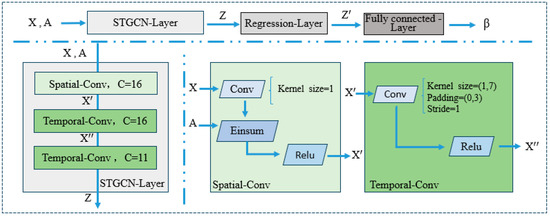
Figure 1.
Structure diagram of the STGCN-PDR model.
The input to the model consists of a feature matrix X and an adjacency matrix A. The feature matrix is defined as follows, where T represents the number of time steps. In this paper, “long” refers to the statistical time period of the stock index data; N represents different nodes, which correspond to various countries and regions in this study; D denotes the features of each node, specifically referring to the relevant characteristics of the stock index in this context. The estimation of the model’s regression coefficients using STGCN-PDR is presented in Algorithm 1 below.
| Algorithm 1: STGCN-PDR |
| 1: Standardize the different sample data. 2: Construct the graph structure. 3: Input: Feature matrix 4: Use spatio-temporal convolutional layers to perform spatial and temporal convolu-tions on the feature matrix to extract spatio-temporal features. 5: Use a regression layer to apply a linear transformation to the output of the spa-tio-temporal graph convolutional layer. 6: Output: Regression coefficient 7: Compute the loss value based on the loss function. 8: Update the model parameters using the optimization algorithm. 9: Repeat steps 4–8 until the maximum number of iterations is reached or convergence criteria are satisfied. |
The detailed steps of parameter estimation are as follows:
Step 1: Standardize the data of different samples. Since the research involves multiple countries and regions with varying levels of development, their dimensions and scales differ significantly. To eliminate inconsistencies in dimensions and scales within the spatio-temporal panel data across different samples, it is necessary to standardize the data first. This paper adopts the Z-score standardization method (Shalabi et al., 2006), as shown in Formula (7):
Here, represents the mean of the j-th feature for the i-th country or region during time period T, and represents the standard deviation of the j-th feature for the i-th country or region during time period T.
Step 2: Construct the graph structure. In this step, each node represents a country or region, and each edge represents the similarity between two countries or regions, denoted as the edge weight. Given that inflation or deflation has a profound impact on investor behavior, and CPI is a commonly used indicator to measure these economic phenomena, this paper uses the cosine similarity of CPI time series for measurement. The calculation formula is referenced in Formula (1), as shown in Formula (8):
Here, x and y represent the CPI time series of different countries or regions, and n indicates the length of the time series. The range of cosine similarity values is [−1, 1], where larger values indicate greater similarity. For each country or region, the cosine similarity between its own CPI time series and itself is set to 0 and used as the self-loop weight. Subsequently, all edge weights and self-loop weights are combined into a symmetric matrix, which forms the adjacency matrix A. As shown in Figure 2, this is a heatmap of the adjacency matrix for 20 countries or regions. Each cell in the matrix represents the cosine similarity of the CPI time series between two countries or regions, with different colors corresponding to different values on the right-hand side.
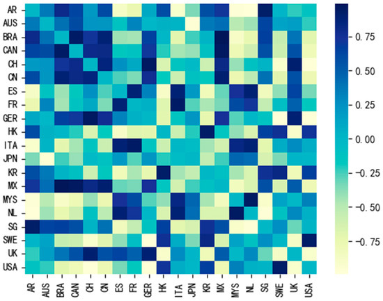
Figure 2.
Heatmap of adjacency matrices among different countries or regions. Note: In this heatmap, the depth of color reflects the similarity between different countries or regions. Darker colors indicate cosine similarity values closer to 1, representing higher similarity between the two countries or regions. Conversely, lighter colors indicate cosine similarity values closer to −1, representing lower similarity between the two countries or regions.
Step 3: The feature matrix X and the adjacency matrix A are used as inputs for the spatio-temporal graph convolutional layer. The output dimension of the spatial convolution layer is set to 16, with a convolution kernel size of 1. For the two temporal convolution layers, their output dimensions are both set to 16, and the convolution kernel size is (1, 7). The model structure is illustrated in Figure 1. The setting of the output layer dimension is based on the principle that a hidden layer with more nodes than the input feature dimension can better extract feature information. However, as the number of hidden layer nodes increases, computational complexity also rises significantly. Therefore, the number of hidden neurons is often set to two-thirds of the input layer size, plus two-thirds of the output layer size, or less than twice the input layer size (Sheela & Deepa, 2013). The configuration of the convolution kernel in the spatial convolution layer reduces the computational load and complexity of the model while enhancing its generalization ability (Dror et al., 2021). For the temporal convolution layer, the convolution kernel is designed to simulate the capability of LSTM in processing time series data, thereby capturing temporal features effectively.
Step 4: Use the regression layer and fully connected layer for coefficient regression and result output. The regression layer is derived from the fully connected layer and serves to map the input feature vector to the output feature vector, achieving multiple linear regression. The output of the spatio-temporal graph convolution layer is taken as the input of the regression layer, with a dimension of . In the regression layer, the tensor is first transposed along the first dimension to become and then reshaped into . Next, a fully connected layer fc1 with an input dimension of and an output dimension of is applied for dimensionality reduction, resulting in a reduced dimension of . Finally, the fully connected layer fc2 outputs the regression coefficient β.
Step 5: Define the loss function and train the model. To estimate the regression coefficients using the neural network, this paper adopts the principle of least squares and transforms the estimation process into the optimization process of the corresponding loss function. Specifically, the loss function is defined by referencing Formula (4), as shown in Formula (9):
Among them, represents the regression coefficient of the j-th feature for the i-th country, and represents the value of the j-th feature of the i-th country at the t-th time point. To prevent overfitting, a regularization term is added to the loss function (Chen et al., 2016), as shown in Formula (10):
Here, is the regularization coefficient. Through the above loss function, during the model training process, minimizing the loss value is set as the optimization objective, thereby achieving the purpose of estimating the regression coefficients. This paper uses the Adam optimizer (Kingma & Ba, 2014) to train the model, with the learning rate determined via the enumeration method. For comparative analysis, this paper constructs two additional regression coefficient estimation models based on CNN and LSTM, namely, CNN-PDR and LSTM-PDR.
4.3. Testing of Parameter Estimation Results
To verify the effectiveness of the parameter estimation method proposed in this paper, the coefficient of determination (R2) (D. B. Zhang, 2017) is adopted as the evaluation index. R2 measures the proportion of the variation in the dependent variable explained by the predictor variables included in the model. The closer its value is to 1, the better the model fits the observed values. For detailed calculation, see Formula (11):
Here, represents the regression sum of squares, which is the sum of the squared differences between the predicted values and the mean. It reflects the variation in the dependent variable that the model can explain. represents the residual sum of squares, which is the sum of the squared differences between the predicted values and the actual values. It reflects the variation in the dependent variable that the model cannot explain. represents the total sum of squares, which is the sum of the squared differences between the actual values and the mean. It reflects the total variation in the dependent variable. Here, denotes the actual value, denotes the mean of the actual values, and denotes the predicted value.
4.4. Risk Prediction of the Model
To verify the accuracy of the proposed parameter estimation model in predicting stock market risks, this paper uses Value-at-Risk (VaR) as the risk measurement indicator and adopts the rolling time window method to predict VaR, which is subsequently compared with the actual return rate. To calculate VaR, it is assumed that the return rate error follows a normal distribution. The formula used for calculation is as follows:
Here, represents the return rate error, represents the inverse cumulative distribution function of the standard normal distribution at the -quantile, and represents the standard deviation of the return rate error. The expected index return rate is shown in Formula (12):
Here, represents the expected index return rate; represents the regression coefficient obtained through training; represents the change rate of gross domestic product; represents the change rate of the consumer price index; represents the change rate of stock returns; represents the change rate of the highest stock price; represents the change rate of the lowest stock price; represents the change rate of the closing price; represents the change rate of the opening price; represents the change rate of the exchange rate; represents the change rate of the previous day’s return rate; represents the change rate of the previous day’s weighted return rate; and represents the current weighted return rate change.
5. Empirical Analysis
To validate the effectiveness of the STGCN-PDR model proposed in this paper, this section performs an empirical analysis using panel data from international stock markets and compares its performance with multiple benchmark models. The analysis encompasses a detailed description of the data sources and features, experimental settings, explanations of the comparison models, and an in-depth evaluation of the model’s prediction accuracy and economic implications.
5.1. Data Sources and Feature Description
The data for this empirical study are sourced from the Refinitiv Eikon database, encompassing daily stock market data from 20 countries and regions, spanning the period from 26 May 2021 to 13 May 2022. These countries and regions include major developed economies such as the United States, China, and the United Kingdom, as well as emerging markets like Malaysia and Brazil. The selection of this time frame is intended to capture the post-pandemic market recovery phase, enabling an assessment of the model’s robustness under conditions of significant market volatility.
To comprehensively characterize the factors influencing stock index fluctuations, this study constructs a multi-dimensional feature system that integrates both macroeconomic and microeconomic indicators. Specifically, the feature set includes the logarithmic return of the previous day, the weighted logarithmic return of the current day, the weighted logarithmic return of the previous day, exchange rates, highest price, lowest price, opening price, closing price, bond interest rates, consumer price index (CPI), and gross domestic product (GDP).
For data processing, to validate the model’s effectiveness, the dataset was split into a training set (26 May 2021–24 January 2022) and a test set (25 January 2022–13 May 2022), with 24 January 2022 as the cutoff point. Additionally, to assess the model’s robustness, based on Asgharian et al.’s (2013) findings regarding the temporal variation of spatial influence and Tamakoshi and Hamori (2014) proposed segmentation method, the dataset was further divided into four stages according to key events that significantly impacted global financial markets. These events include the Afghanistan crisis on 16 August 2021, which caused sharp fluctuations in global financial markets; the Russia–Ukraine crisis on 24 February 2022, which triggered widespread market panic; and the global financial “Black Monday” on 12 April 2022, during which the Dow Jones Index in the U.S. plummeted by nearly 10%. The four stages are defined as follows: Stage 1 (27 May 2021–15 August 2021), Stage 2 (16 August 2021–23 February 2022), Stage 3 (24 February 2022–12 April 2022), and Stage 4 (13 April 2022–3 May 2022). This multi-stage division is grounded in granularity theory, which simulates the human strategy of observing complex problems at different levels of detail. The primary advantage of applying this theory is that it ensures uniform sampling over extended periods while minimizing computational costs. Subsequently, for each stage, the datasets were further partitioned into training and test sets using an 80% time step ratio.
Due to space constraints, Table 1 provides partial stock index feature information for the United States (USA), China (CN), the United Kingdom (UK), and France (FR) as of 17 May 2021.

Table 1.
Feature information of stock indices in selected countries.
5.2. Comparative Analysis of Model Parameter Estimation Results
The essence of deep learning lies in the process of inductive reasoning from data. Any deep learning model inherently involves uncertainty. D’Amour et al. (2022) demonstrated through multi-domain empirical studies, including computer vision, medical imaging, natural language processing, and electronic medical record prediction, that even minor changes in random initialization, hyperparameters, or optimization details can lead to significant differences in model performance under external distribution shifts, bias tests, and stress tests. This instability and irreproducibility of results persist even when the training and deployment distributions are consistent, due to “arbitrary choices” made during the training process. Such issues undermine the credibility and interpretability of deep learning models in high-risk scenarios. While tolerable in tasks focusing on “point value prediction”, these challenges become critical in regression parameter interpretation contexts, where even minor weight drifts can significantly alter economic meaning interpretation and risk measurement, thereby weakening the model’s policy or investment usability. Therefore, while this paper proposes STGCN-PDR to address the “coefficient invisibility” issue of traditional neural networks, it is also essential to evaluate the robustness and reverse quantification of its parameter estimation to provide confidence boundaries for subsequent risk management.
To systematically assess the trade-off between fitting accuracy and the robustness of STGCN-PDR and two control models—LSTM-PDR and CNN-PDR—under random perturbations, the study conducts 1000 independent convergence training sessions for each model across the full sample (181 days) and four phased samples (52, 110, 27, and 18 days). Each experiment employs random weight initialization and records the mean R2 (), standard deviation of R2 (), and coefficient of variation (CV) for each model at different training rounds. CV serves as a relative fluctuation index that normalizes absolute dispersion to the mean scale, making it suitable for comparing the robustness of different models with consistent dimensions but varying mean levels (Shechtman, 2001). Additionally, to examine computational costs, the average training time per round is also recorded. All experiments were conducted in a uniform hardware environment (Intel Core i5-8300H @ 2.30 GHz, 8 GB RAM, Intel Corporation, Santa Clara, CA, USA).
To comprehensively capture the entire training trajectory of the models from “underfitting → convergence → mild overfitting”, this paper evaluates their performance at 500, 1000, 1500, 2000, and 2500 rounds, with increments of 500 rounds. Preliminary experiments indicate that all three models remain in a rapid growth phase at 500 rounds; the growth rate significantly decelerates after 1500 rounds; and by 2500 rounds, the training and validation losses tend to stabilize, with some models exhibiting mild overfitting. Below, we systematically analyze the performance differences of the three models based on the A, B, and C metrics across these grid-based rounds. Comprehensive results are summarized in Table 2, Table 3, Table 4, Table 5 and Table 6.
Table 2.
Comparison of model performance across the entire time period.
Table 3.
Comparison of model performance in the first time period.
Table 4.
Comparison of model performance in the second time period.
Table 5.
Comparison of model performance in the third time period.
Table 6.
Comparison of model performance in the fourth time period.
As shown in Table 2 (complete sample), the performance of each model across different training rounds can be categorized into three stages: early (500–1000 rounds), middle (1500 rounds), and late (2000–2500 rounds).
In the early training stage (500 and 1000 rounds), CNN-PDR achieved the highest R2 values (0.5300 and 0.6579), with relatively low standard deviations of 0.0587 and 0.0420, which were lower than those of LSTM-PDR (0.0667 and 0.0560) and STGCN-PDR (0.0691 and 0.0508). This indicates that the convolutional kernel’s ability to rapidly capture local correlations enables CNN-PDR to achieve both high accuracy and moderate robustness. Additionally, due to its relatively simple architecture, parameter tuning and optimization for CNN are more intuitive and efficient, allowing it to quickly converge to an optimal parameter configuration during the early training phase (Alzubaidi et al., 2021).
In the middle training stage (1500 rounds), as the number of training rounds increased, CNN-PDR continued to maintain the highest value ( = 0.6936). However, at this stage, both STGCN-PDR ( = 0.6898) and LSTM-PDR ( = 0.6750) demonstrated faster convergence rates, rapidly approaching the performance level of CNN-PDR.
In the late training stage, at 2000 rounds, STGCN-PDR achieved the highest value (0.6981) under the same number of training rounds, with the smallest standard deviation ( = 0.0102). At this point, the value of CNN-PDR was slightly lower (0.6980), and its standard deviation (0.0183) increased compared to the middle stage (1500 rounds). This result may stem from the fact that STGCN, by integrating graph convolution (GCN) and temporal convolution (TCN), has a more complex structure than CNN. Consequently, it requires additional training rounds to reach its optimal performance. Furthermore, STGCN’s superior ability to simultaneously capture spatial and temporal dependencies (Wu et al., 2020) contributes to its enhanced performance relative to CNN-PDR.
Then, at 2500 training rounds, although LSTM-PDR achieved the best values ( = 0.6988, ) among all models across all stages, its average training time of 318 s was significantly longer than that of STGCN-PDR (83.3414 s). Moreover, compared to STGCN-PDR and CNN-PDR at 2000 rounds, the improvement in R2 performance for LSTM-PDR was not substantial. The likely reason is that while LSTM can effectively capture long-term dependencies through its specialized gating mechanism (Van Houdt et al., 2020), the substantially increased training time also highlights a limitation of the model. Additionally, it is noteworthy that both STGCN-PDR and CNN-PDR exhibited varying degrees of performance degradation at 2500 rounds compared to 2000 rounds, specifically characterized by a decrease in values and an increase in the standard deviation . This suggests that these two models experienced differing levels of overfitting. Therefore, their optimal number of training rounds is approximately 2000, which also implies that LSTM-PDR exhibits slower convergence during model training.
In summary, CNN-PDR demonstrates rapid convergence in the early stages; STGCN-PDR achieves the best balance between “accuracy” and “robustness” with the lowest computational cost at around 2000 rounds; although LSTM-PDR can marginally enhance performance with additional training rounds, this comes at the expense of significantly higher time consumption, indicating its limited suitability for resource-constrained scenarios.
From the model performance results of the four sub-periods (52 days, 110 days, 27 days, and 18 days) shown in Table 3, Table 4, Table 5 and Table 6, each model demonstrates a similar overall trend to the full period while showing varying degrees of differences in specific aspects such as accuracy (), robustness (), and training efficiency.
Firstly, from the perspective of prediction accuracy (), STGCN-PDR shows a significant advantage in the vast majority of sub-periods. For instance, in the first period (52 days), the values of STGCN-PDR at 1500 rounds (0.5666), 2000 rounds (0.5801), and 2500 rounds (0.5832) are all higher than those of LSTM-PDR (0.5389, 0.5722, 0.5817). In the second period (110 days), the values of STGCN-PDR at 1500 rounds (0.6925) and 2000 rounds (0.7073) also exceed those of CNN-PDR (0.6901, 0.6843) and LSTM-PDR (0.6706, 0.7007). In the third period (27 days), STGCN-PDR achieves the highest value (0.3256) at 500 rounds, which is higher than that in LSTM-PDR ( = 0.3102) and CNN-PDR ( = 0.2650); although there is a decline in accuracy at higher rounds, it still shows a clear advantage in the early stage. In the fourth period (18 days), the values of STGCN-PDR at 1000 rounds (0.3304), 1500 rounds (0.3983), and 2000 rounds (0.4393) are all higher than those of CNN-PDR ( = 0.3170, 0.3132, 0.3035) and LSTM-PDR ( = 0.3218, 0.3816, 0.4307), fully demonstrating that the STGCN-PDR model still has good generalization ability for short sample data.
Secondly, in terms of the robustness of the model’s prediction results (coefficient of variation ), STGCN-PDR also demonstrated a clear advantage in most sub-periods. In the first sub-period (52 days) at 2000 rounds, the value of STGCN-PDR reached 0.0183, which was lower than that of CNN-PDR ( = 0.0309) and LSTM-PDR ( = 0.0294). In the second sub-period (110 days) at 1500 and 2000 rounds, the values of STGCN-PDR were 0.0365 and 0.0443, respectively, significantly lower than those of CNN-PDR (0.0906 and 0.1885). In the third sub-period (27 days), although all models were constrained by the short sample size and showed high variance, the value of STGCN-PDR at 500 rounds (0.0731) was still much lower than that of CNN-PDR (2.8143), and it maintained relatively stable values at 1000 rounds (0.0534) and 1500 rounds (0.2998). In the fourth sub-period (18 days), although the value of STGCN-PDR was relatively high at the initial stage (500 rounds) (0.8301), it significantly decreased to 0.3000 at 1500 rounds and 0.2761 at 2000 rounds, while the values of CNN-PDR at the corresponding rounds (0.8142 and 1.2913) remained high, indicating that the robustness of STGCN-PDR after deep training was superior to that of the CNN-PDR model.
Thirdly, from the perspective of computational efficiency, STGCN-PDR showed significant computational advantages in all four sub-samples. For example, in the first period (52 days) at 2500 rounds, the average training time of STGCN-PDR was 31.3530 s, significantly lower than that of LSTM-PDR (88.4740 s); in the second period (110 days) at 2500 rounds, the training time of STGCN-PDR was 53.7250 s, lower than that of LSTM-PDR (172.9782 s); in the third (27 days) and fourth (18 days) periods, the training times of STGCN-PDR (18.6893 s and 15.0630 s) were also significantly lower than those of LSTM-PDR (49.2420 s and 33.5225 s), demonstrating a clear training efficiency advantage.
Furthermore, although CNN-PDR showed high accuracy in the initial training stages (500–1000 rounds) of each phase, as the number of training rounds increased, its accuracy advantage was gradually caught up with and even surpassed by STGCN-PDR and LSTM-PDR, and its variance rapidly expanded, showing obvious instability. For instance, in the second phase (110 days) at 2000 rounds, the value of CNN-PDR was 0.1885, much higher than that of STGCN-PDR (0.0443) and LSTM-PDR (0.0247) at the same time; in the third phase (27 days) at 500 rounds, the value of CNN-PDR was as high as 2.8143, further highlighting the problem of uncontrollable variance in short time series data.
In conclusion, based on a comprehensive comparison across the four sub-sample stages, STGCN-PDR demonstrated the most prominent performance in terms of prediction accuracy, robustness, and computational efficiency. Specifically, its training performance reached an optimal level around 2000 rounds, indicating that STGCN-PDR is capable of effectively capturing the characteristics of spatio-temporal data with varying lengths and achieving stable and efficient parameter estimation. While LSTM-PDR exhibits certain robustness advantages in extremely short time windows, this comes at the cost of high computational demands, which limits its generalization ability in practical applications. Although CNN-PDR possesses the fastest training speed, its significant decline in accuracy and pronounced variance fluctuations substantially reduce its applicability in practical risk management scenarios. Therefore, considering the combined factors of accuracy, robustness, and computational efficiency, STGCN-PDR remains the preferred model for addressing regression problems involving spatio-temporal panel data.
5.3. Analysis of the Model’s Prediction Results
To ensure that the model achieves stable predictive performance, this study adopts methodology in X. Zhang et al. (2022) for selecting effective training samples and employs R2 as a criterion for evaluating the model’s training outcomes. Specifically, the number of training rounds required for the stabilization of the mean R2 is first identified and set as the final training round. Subsequently, model outputs with R2 values close to the stabilized mean R2 are selected as the effective regression coefficients for Value-at-Risk (VaR) detection. This approach aims to maintain consistent model performance during the prediction phase, thereby providing a robust parameter foundation for subsequent VaR-based risk assessments.
Table 7 illustrates the VaR backtest results of the rolling time window based on 181 time steps for four models: general linear regression, CNN-PDR, LSTM-PDR, and STGCN-PDR. The table displays the mean values of the significance p-values and corresponding statistics across 79 VaR backtests. The figures outside the parentheses represent the test statistics, while those inside the parentheses denote the p-values. In the UC, IND, and CC tests, smaller test statistics (or larger p-values) indicate better performance. According to Kupiec (1995) and Candelon et al. (2011), if the p-value exceeds 0.05, the prediction result cannot be rejected. From the results, it is evident that the STGCN-PDR model achieves the largest p-values in the UC, IND, and CC tests across all confidence levels, suggesting that its VaR predictions exhibit the highest credibility. Notably, at the 99% confidence level, the p-values of the UC, IND, and CC tests for the STGCN-PDR model are significantly higher than those of the other three models, indicating its robust reliability even under extreme conditions.
Table 7.
Backtesting results of VaR.
Furthermore, at all confidence levels, the p-values of the UC, IND, and CC tests for the LSTM-PDR model surpass those of the CNN-PDR and general linear regression models. This highlights the limitations of ordinary regression models in effectively capturing spatio-temporal features from the data. Compared with STGCN-PDR, LSTM-PDR demonstrates a strong ability to extract temporal features from stock index panel data but exhibits some inadequacy in capturing spatial features.
To further analyze the stability and timeliness of the models’ performance, the evaluation to different time periods are extended. Table 8, Table 9, Table 10 and Table 11 below provide the VaR backtesting results based on different models across four time periods. These results differ from those presented in Table 7. As shown in Table 8, during the first time period, the STGCN-PDR model achieves the largest p-values in the CC test at the 95% and 90% confidence levels, with values of 0.18346 and 0.37307, respectively. Additionally, it attains the highest p-values in the IND test across all confidence levels, specifically 0.57006, 0.57666, and 0.54897. Surprisingly, the general linear regression model exhibits the largest p-values in the UC test across all confidence levels, with values of 0.09238, 0.18934, and 0.35817. This indicates that both models yield valid predictions during the first time period. A possible explanation is that the general linear regression model performs well within relatively short time spans. However, this does not imply that the general linear regression model will exhibit strong predictive performance in complex international financial environments. Neural networks typically require large datasets to achieve optimal results, and insufficient data may hinder the model’s ability to fully capture the spatio-temporal characteristics of stock index data, thereby reducing prediction accuracy.
Table 8.
Backtesting results for VaR in the first time period.
Table 9.
Backtesting results for VaR in the second time period.
Table 10.
Backtesting results for VaR in the third time period.
Table 11.
Backtesting results for VaR in the fourth time period.
As observed in Table 9, during the second time period, the STGCN-PDR model achieves the largest p-values in the CC test at the 99% and 95% confidence levels, with values of 0.30758 and 0.89367, respectively. This suggests that the STGCN-PDR model demonstrates the most effective predictive performance during this time period. The extended time span likely provides more data for learning and prediction, enabling neural network models to outperform general linear models.
From Table 10 and Table 11, it can be seen that during the third and fourth time periods, the results of the UC and CC tests for all models across all confidence levels reject the null hypothesis, indicating that the predictions of all models are invalid. This may result from the short time spans and limited data volumes in these periods, which prevent the models from effectively estimating regression coefficients.
To visually validate the model performance and complement the statistical results in Table 8, Table 9, Table 10 and Table 11, comparisons of VaR predictions with actual returns across different time periods are conducted. Figure 3 illustrates the comparison of VaR and actual returns for different models across various time periods. In Figure 4, the blue line represents the actual logarithmic return, the orange line corresponds to the VaR based on the STGCN-PDR model, the green line corresponds to the VaR based on the CNN-PDR model, the red line corresponds to the VaR based on the LSTM-PDR model, and the purple line corresponds to the VaR based on the general linear regression model.
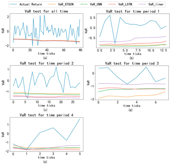
Figure 3.
Comparison of VaR and actual returns at different time periods. Note: This figure shows the comparison between the rolling VaR of four models and the actual returns. Both VaR and actual returns are averaged over 20 countries. (a–e) represent the full time period, the first time period, the second time period, the third time period, and the fourth time period, respectively. The time window size is the size of the training set, and the number of rolling times is the size of the test set. The confidence level of VaR is 95%. The horizontal axis represents the number of rolling times, and the vertical axis represents VaR.
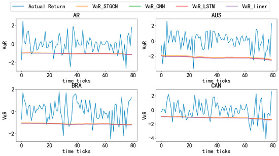
Figure 4.
Comparison of VaR and actual returns in different countries (1). Note: The figure shows the comparison of VaR and actual returns of different models in 20 countries over the entire time period, with a confidence level of 95%.
In the complete time period (a), the orange line surpasses the others, indicating that the STGCN-PDR-based VaR prediction method performs better due to its consideration of spatial correlation. During the first time period (b), the purple line aligns most closely with the actual values, suggesting that the other three neural network-based models perform worse than the general linear regression model. This finding aligns with Table 8, implying that insufficient data may cause neural network models to underperform compared to the general linear regression model. Additionally, the red line surpasses the orange and green lines, potentially because LSTM’s recurrent network structure enhances its performance in short-term prediction tasks (Van Houdt et al., 2020). During the second time period (c), the orange line remains at the top. In the third time period (d), all models’ VaR results deviate significantly from the actual values, consistent with the findings in Table 10. During the fourth time period (e), the orange line aligns most closely with the actual values.
Figure 4, Figure 5, Figure 6, Figure 7 and Figure 8 compare the actual logarithmic returns (blue line) and VaR (lines of other colors) of different countries’ stock markets based on various models at a 95% confidence level. As shown in the Figure 4, Figure 5, Figure 6, Figure 7 and Figure 8, the VaR of the STGCN-PDR model (orange line) surpasses that of other models in nearly all countries, demonstrating its superior performance in predicting stock market returns across different countries.
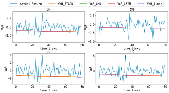
Figure 5.
Comparative analysis of VaR and actual returns across different countries (2). Note: This figure presents a detailed comparison of Value-at-Risk (VaR) and actual returns for various models across 20 countries over the entire time period, with a confidence level set at 95%.
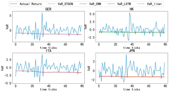
Figure 6.
Comparative analysis of VaR and actual returns across different countries (3). Note: This figure provides an in-depth analysis of Value-at-Risk (VaR) and actual returns for different models across 20 countries over the entire time period, maintaining a confidence level of 95%.
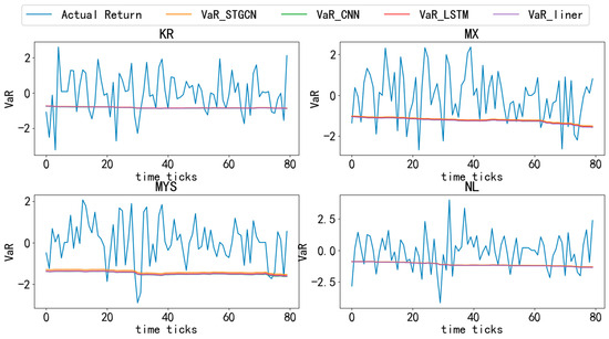
Figure 7.
Comparative analysis of VaR and actual returns across different countries (4). Note: This figure provides a comparative analysis of Value-at-Risk (VaR) and actual returns for various models across 20 countries over the entire time period, with a confidence level set at 95%.
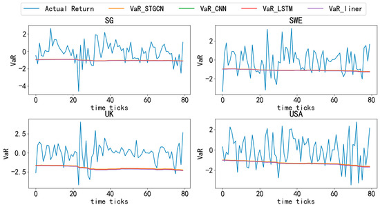
Figure 8.
Comparative analysis of VaR and actual returns across different countries (5). Note: This figure presents an in-depth comparison of Value-at-Risk (VaR) and actual returns for different models across 20 countries over the entire time period, maintaining a confidence level of 95%.
In summary, the STGCN-PDR model exhibits robust and accurate VaR predictions across different confidence levels. This may be attributed to its ability to effectively capture the spatio-temporal correlations of stock index data, enhancing the quality of VaR predictions. These findings validate the application value of the STGCN-PDR model in financial risk management.
Furthermore, (1) prediction lines tend to appear as relatively smooth straight lines, whereas actual investment returns exhibit more pronounced fluctuations. This occurs because, in the VaR prediction process, stock market index returns are primarily influenced by macroeconomic variables, which change minimally in the short term. Due to space constraints in this article, Figure 2 and Figure 4 only present VaR prediction results at the 95% confidence level. However, the prediction conclusions remain valid at the 90% and 99% confidence levels, as supported by the data in Table 7, Table 8, Table 9, Table 10 and Table 11.
5.4. Application Analysis of the STGCN-PDR Model
Regression coefficients vary across countries, potentially reflecting differences in economic environments, policies, and market structures. These variations directly influence the sensitivity of stock index returns to various economic indicators. Notably, the regression coefficients for CPI are consistently negative across all countries. This may be attributed to the fact that inflation (i.e., an increase in CPI) tends to lead to a decline in actual stock index returns. Conversely, an increase in economic activity (i.e., higher GDP) is associated with rising stock index returns, indicating a negative correlation between CPI and stock index returns. Furthermore, the day-of-market conditions (WRt, close, open, and low) exert the most significant impact on stock index returns, particularly the opening and closing prices. This suggests that immediate market dynamics have a stronger influence on stock index returns compared to long-term economic indicators. Collectively, these findings provide valuable insights into the relationship between stock index returns and various economic indicators across different countries.
Consequently, the STGCN-PDR model proposed in this study has been empirically validated as effective for coefficient regression and risk prediction on spatio-temporally correlated international equity index panel data, offering robust decision-making support for international investors.
This paper deliberately focuses on international equities to enable a deep, well-identified evaluation of STGCN-PDR under heterogeneous regimes and multi-country dependencies. The architecture, however, is market agnostic by construction: (i) the graph layer encodes cross-sectional linkages that can be rebuilt for each asset class; (ii) temporal convolutions capture regime-dependent dynamics shared by many financial markets (e.g., volatility clustering, heavy tails); and (iii) the embedded regression head preserves coefficient-level interpretability and uncertainty summaries across feature sets. Consistent with these design arguments, recent evidence shows that spatio-temporal GNNs and modern deep architectures improve forecasting outside equities—e.g., in commodities when inter-asset spillovers are explicitly modeled (Foroutan & Lahmiri, 2024) and in foreign exchange when multivariate cross-series information is fed to state-of-the-art sequence models (Fischer et al., 2024). In fixed income, graph-structured learning on bond networks has enhanced price/yield prediction, indicating that relational graphs are informative beyond equities (D. Zhou et al., 2022). Taken together, the structural commonalities in data-generating processes and the graph-based design of STGCN-PDR provide evidence-informed portability rather than a claim already tested here. We therefore frame multi-asset validation (bonds, FX) as a natural next step of the research agenda—implementing market-specific adjacency designs (e.g., maturity/issuer proximity for bonds, currency triangle consistency and macro linkages for FX) and decision-oriented backtests (e.g., VaR breaches and risk budgeting) to quantify portability (Foroutan & Lahmiri, 2024; Fischer et al., 2024; D. Zhou et al., 2022).
Thus, while this study primarily focuses on the stock market, the STGCN-PDR model demonstrates structural features that make it potentially extendable to the bond and foreign exchange markets. This provides a promising direction for future research, where the model could be further validated and applied to other spatio-temporally correlated financial markets.
5.5. Discussion
5.5.1. Testing of the Research Hypotheses
H1: On the full sample, STGCN-PDR attains the highest mean R2 after 2000 epochs (0.6981) and surpasses LSTM-PDR from approximately 1500 epochs onward (0.6898 vs. 0.6750; Table 2). The advantage persists across sub-period analyses (Table 3, Table 4, Table 5 and Table 6). In the second sub-period (110 days; Table 4), the R2 of STGCN-PDR at 1500 and 2000 epochs (0.6925, 0.7073) is materially higher than that of the competing models. The graphical diagnostics are consistent with these results: the VaR path in Figure 3a aligns most closely with realized returns, and cross-country prediction errors are comparatively smaller (Figure 4, Figure 5, Figure 6, Figure 7 and Figure 8). These findings indicate that the spatio-temporal graph convolutions effectively capture nonlinear inter-market dependence, thereby improving predictive accuracy relative to linear and deep learning baselines without explicit graph structure. Hence, H1 is supported.
H2: Statistical robustness is evidenced by the lowest coefficient of variation (CV) of R2 for STGCN-PDR in the full sample at 2000 epochs (CV = 0.0102; Table 2), compared with CNN-PDR (0.0183) and LSTM-PDR (0.0150). Sub-period results are consistent: in the second period (110 days), STGCN-PDR exhibits markedly lower CVs than CNN-PDR at both 1500 and 2000 epochs; in the third period (27 days), characterized by heightened volatility, the CV of CNN-PDR escalates to 2.8143, whereas STGCN-PDR remains in a moderate range (e.g., 0.0731 at 500 epochs; Table 5). Regarding interpretability, the embedded regression layer yields economically coherent coefficients (Table 12): CPI growth enters with a negative sign across countries, consistent with inflation compressing margins and raising discount rate uncertainty, while GDP growth enters positively, consistent with improved earnings prospects and confidence channels. Therefore, H2 is supported.
Table 12.
Coefficient regression results of the STGCN-PDR model for selected countries.
H3: With respect to efficiency, the average training time for STGCN-PDR is of the same order as CNN-PDR yet far below LSTM-PDR on the full sample (e.g., 67.1 s vs. 63.2 s vs. 248.8 s at 2000 epochs; Table 2). Sub-period evidence is concordant: at 2500 epochs, STGCN-PDR vs. LSTM-PDR training time equals 31.3530 s vs. 88.4740 s (first period, 52 days), 53.7250 s vs. 172.9782 s (second, 110 days), 18.6893 s vs. 49.2420 s (third, 27 days), and 15.0630 s vs. 33.5225 s (fourth, 22 days). In terms of stability across regimes, STGCN-PDR generally attains optimal or near optimal accuracy, with comparatively low CVs in most periods (Table 3, Table 4, Table 5 and Table 6), including under distributional stress (third period). Hence, H3 is supported.
5.5.2. Economic Interpretation and Practical Implications
The sign and magnitude patterns of the embedded regression coefficients (Table 12) are consistent with macro-financial mechanisms. A negative association between CPI growth and predicted risk aligns with the view that persistent inflation erodes real cash flows and increases discount rate uncertainty, thereby aggravating return volatility. Conversely, positive GDP growth coefficients indicate that improving macro conditions mitigate downside risk through stronger earnings prospects and confidence channels. Cross-country heterogeneity in coefficient magnitudes plausibly reflects differences in monetary policy stances, market depth, and trade linkages—dimensions parsimoniously encoded via the graph adjacency that mediates spillovers among markets.
For practitioners, two implications follow. First, the coefficient paths provide transparent signals for risk budgeting and dynamic hedging: when inflation factors dominate (more negative CPI coefficients), higher volatility target scaling or option overlays are warranted. Second, the graph-based propagation captured by STGCN-PDR permits early detection of regional stress transmission, informing cross-market allocation and overlay hedges.
5.5.3. Robustness and Sensitivity Analyses
Three aspects merit emphasis. (i) Run-to-run stability. Consistently lower CVs for STGCN-PDR across epochs and sub-periods indicate that its estimates are less sensitive to random initialization than those from CNN-PDR and LSTM-PDR (Table 2, Table 3, Table 4, Table 5 and Table 6). (ii) Regime sensitivity. Under the high-volatility third period (27 days; Table 5), dispersion increases sharply for CNN-PDR (CV = 2.8143), whereas STGCN-PDR remains comparatively contained (e.g., CV = 0.0731 at 500 epochs), suggesting greater resilience to distributional shifts. (iii) Computational sensitivity. Given the substantially reduced training time relative to LSTM-PDR (Table 2 and sub-period summaries), model selection and hyperparameter tuning can be performed more extensively for STGCN-PDR within the same computational budget, which further improves out-of-sample reliability.
5.5.4. Limitations and Directions for Future Research
This study has limitations. First, the adjacency specification is exogenously imposed; while the baseline captures salient cross-market linkages, alternative constructions (e.g., time-varying, partial-correlation, or information flow graphs) may refine propagation channels, especially during crises. Second, although repeated runs quantify parameter-estimation uncertainty, the treatment remains frequentist; a fully probabilistic formulation (e.g., Bayesian deep GNN) could yield interval-valued coefficient paths. Third, evaluation focuses on risk prediction accuracy (e.g., R2 and VaR curves); incorporating decision-oriented utility criteria (e.g., volatility-targeted portfolio outcomes or downside risk penalties) would strengthen economic validation. Finally, given potential structural breaks, extending the architecture with regime-switching or attention-based components may further enhance robustness.
6. Conclusions
This study develops a spatio-temporal graph convolutional regression framework (STGCN-PDR) for international equity risk prediction. By combining graph-based spatial convolutions and temporal convolutions with an embedded regression layer, the model jointly captures cross-market dependencies and time-varying dynamics while preserving coefficient-level interpretability. The framework, therefore, bridges the traditional trade-off between predictive performance and economic interpretability in high-dimensional financial settings.
Empirically, the evidence aligns with all three hypotheses. Accuracy (H1): on the full sample and across multiple sub-periods, STGCN-PDR attains higher R2 than linear and non-graph deep learning baselines, with particularly strong performance in the second sub-period and consistent graphical diagnostics (Figure 3; Table 3, Table 4, Table 5 and Table 6). Robustness and interpretability (H2): repeated-run analyses show lower coefficients of variation for R2 and economically coherent signs for country-level coefficients (negative CPI, positive GDP; Table 12). Efficiency and generalizability (H3): training times are materially lower than those of LSTM-based benchmarks, and performance remains comparatively stable under distributional stress (e.g., the third sub-period). Together, these results indicate that explicitly encoding cross-market linkages on a graph, coupled with a regression head, yields a favorable accuracy–robustness–efficiency profile.
From a practical perspective, the model provides operational VaR forecasts and transparent coefficient paths that support risk budgeting, dynamic hedging, and cross-border stress surveillance. The graph structure facilitates early detection of regional propagation, informing cross-market allocation and overlay hedges. These properties make STGCN-PDR a viable tool for investors and regulators seeking timely, interpretable, and scalable risk assessment.
The study also highlights avenues for continued improvement. First, complementing goodness-of-fit with error-based metrics (e.g., MAE, RMSE) would broaden evaluation. Second, allowing coefficients to evolve dynamically could better accommodate regime shifts. Third, modeling heavy-tailed return distributions—or adopting non-/semi-parametric approaches—may enhance tail-risk measurement. Fourth, extending the framework to high-frequency data would enable intraday surveillance and further test scalability. Finally, exploring time-varying or information flow graphs could refine how cross-market linkages are represented, especially during crises.
Author Contributions
Conceptualization, G.M. and C.T.; methodology, W.J.; software, W.J.; validation, G.M., W.Z. and J.R.; formal analysis, J.R.; investigation, G.M.; resources, G.M.; data curation, W.J.; writing—original draft preparation, W.J. All authors have read and agreed to the published version of the manuscript.
Funding
This research was funded by [the National Natural Science Foundation of China] grant numbers [72161001, 71963001, U1901223], Key Research Base of Humanities and Social Sciences in Guangxi Universities Guangxi Development Research Strategy Institute (2024GDSIYB10). And The APC was funded by [Chi-na-Asean School of Economics (No. 2024JK16)].
Institutional Review Board Statement
Not applicable.
Informed Consent Statement
Not applicable.
Data Availability Statement
No new data were created or analyzed in this study. Data sharing is not applicable to this article.
Acknowledgments
The authors thank the reviewers, Associate Editor, Copy Editor, and Editor for helpful comments and suggestions that improved the manuscript in a substantial way.
Conflicts of Interest
The authors declare no conflicts of interest.
References
- Akbari Asanjan, A., Yang, T., Hsu, K., Sorooshian, S., Lin, J., & Peng, Q. (2018). Short-term precipitation forecast based on the PERSIANN system and LSTM recurrent neural networks. Journal of Geophysical Research: Atmospheres, 123(22), 12543–12563. [Google Scholar] [CrossRef]
- Alzubaidi, L., Zhang, J., Humaidi, A. J., Al-Dujaili, A., Duan, Y., Al-Shamma, O., Santamaría, J., Fadhel, M. A., Al-Amidie, M., & Farhan, L. (2021). Review of deep learning: Concepts, CNN architectures, challenges, applications, future directions. Journal of Big Data, 8(1), 53. [Google Scholar] [CrossRef] [PubMed]
- Asgharian, H., Hess, W., & Liu, L. (2013). A spatial analysis of international stock market linkages. Journal of Banking & Finance, 37(12), 4738–4754. [Google Scholar] [CrossRef]
- Bollerslev, T. (1986). Generalized autoregressive conditional heteroscedasticity. Journal of Econometrics, 31(3), 307–327. [Google Scholar] [CrossRef]
- Box, G. E. P. (2013). Box and Jenkins: Time series analysis, forecasting and control. In A very British affair (pp. 123–156). Palgrave Advanced Texts in Econometrics. Palgrave Macmillan. [Google Scholar] [CrossRef]
- Breiman, L. (2001). Random forests. Machine Learning, 45(1), 5–32. [Google Scholar] [CrossRef]
- Candelon, B., Colletaz, G., Hurlin, C., & Tokpavi, S. (2011). Backtesting value-at-risk: A GMM duration-based test. Journal of Financial Econometrics, 9(2), 314–343. [Google Scholar] [CrossRef]
- Chen, Y., Jiang, H., Li, C., Jia, X., & Ghamisi, P. (2016). Deep feature extraction and classification of hyperspectral images based on convolutional neural networks. IEEE Transactions on Geoscience and Remote Sensing, 54(10), 6232–6251. [Google Scholar] [CrossRef]
- Chen, Y., Li, F., Deng, Z., Chen, X., & He, J. (2017). PM2.5 forecasting with hybrid LSE model-based approach. Software Practice and Experience, 47(3), 379–390. [Google Scholar] [CrossRef]
- Cortes, C., & Vapnik, V. (1995). Support-vector networks. Machine Learning, 20(3), 273–297. [Google Scholar] [CrossRef]
- Cui, F. L., Chai, Y. D., Jiang, Y. C., Qian, Y., Sun, J., & Liu, Y. (2025). Online doctor recommendation method considering uncertainty of deep learning models. Chinese Journal of Management Science. Advance online publication. [Google Scholar] [CrossRef]
- D’Amour, A., Heller, K., Moldovan, D., Adlam, B., Alipanahi, B., Beutel, A., Chen, C., Deaton, J., Eisenstein, J., Hoffman, M. D., Hormozdiari, F., Houlsby, N., Hou, S., Jerfel, G., Karthikesalingam, A., Lucic, M., Ma, Y., McLean, C., Mincu, D., … Sculley, D. (2022). Underspecification presents challenges for credibility in modern machine learning. Journal of Machine Learning Research, 23(226), 1–61. Available online: https://jmlr.org/papers/v23/20-1335.html (accessed on 25 August 2025).
- Dimitrakopoulos, R., & Luo, X. (1994). Spatiotemporal modelling: Covariances and ordinary Kriging systems. In Geostatistics for the next century (pp. 88–93). Springer. [Google Scholar]
- Dror, A. B., Zehngut, N., Raviv, A., Artyomov, E., Vitek, R., & Jevnisek, R. J. (2021). Layer folding: Neural network depth reduction using activation linearization. In Proceedings of the British machine vision conference (pp. 1–12). BMVA Press. [Google Scholar]
- Engle, R. F. (1982). Autoregressive conditional heteroscedasticity with estimates of the variance of United Kingdom inflation. Econometrica, 50, 987–1007. [Google Scholar] [CrossRef]
- Fan, G. F., Zhang, R. T., Cao, C. C., Peng, L. L., Yeh, Y. H., & Hong, W. C. (2024). The volatility mechanism and intelligent fusion forecast of new energy stock prices. Financial Innovation, 10(1), 84. [Google Scholar] [CrossRef]
- Farrell, M. H., Liang, T., & Misra, S. (2021). Deep neural networks for estimation and inference. Econometrica, 89(1), 181–213. [Google Scholar] [CrossRef]
- Fischer, T., Sterling, M., & Lessmann, S. (2024). FX-spot predictions with state-of-the-art transformer and time embeddings. Expert Systems with Applications, 249, 123538. [Google Scholar] [CrossRef]
- Foroutan, P., & Lahmiri, S. (2024). Deep learning-based spatial-temporal graph neural networks for price movement classification in crude oil and precious metal markets. Machine Learning with Applications, 16, 100552. [Google Scholar] [CrossRef]
- Gal, Y., & Ghahramani, Z. (2016). Dropout as a Bayesian approximation: Representing model uncertainty in deep learning. In Proceedings of the 33rd international conference on machine learning (pp. 1050–1059). JMLR.org. [Google Scholar]
- Glorot, X., Bordes, A., & Bengio, Y. (2011, April 11–13). Deep sparse rectifier neural networks (Proceedings of Machine Learning Research). Fourteenth International Conference on Artificial Intelligence and Statistics (Vol. 15, pp. 315–323), Fort Lauderdale, FL, USA. Available online: https://proceedings.mlr.press/v15/glorot11a.html (accessed on 25 August 2025).
- Gu, S., Kelly, B., & Xiu, D. (2020). Empirical asset pricing via machine learning. The Review of Financial Studies, 33(5), 2223–2273. [Google Scholar] [CrossRef]
- Hassoun, M. H. (1995). Fundamentals of artificial neural networks. MIT Press. [Google Scholar]
- Kingma, D. P., & Ba, J. L. (2014). Adam: A method for stochastic optimization. arXiv. arXiv:1412.6980. [Google Scholar]
- Kupiec, P. H. (1995). Techniques for verifying the accuracy of risk measurement models. The Journal of Derivatives, 3(2), 73–84. [Google Scholar] [CrossRef]
- Liao, H. C., & Xu, Z. S. (2015). Approaches to manage hesitant fuzzy linguistic information based on the cosine distance and similarity measures for HFLTSs and their application in qualitative decision making. Expert Systems with Applications, 42(12), 5328–5336. [Google Scholar] [CrossRef]
- Lu, J., Zhang, Q., Yang, Z., Tu, M., Lu, J., & Peng, H. (2019). Short-term load forecasting method based on CNN-LSTM hybrid neural network model. Automation of Electric Power Systems, 43(8), 131–137. [Google Scholar] [CrossRef]
- Martin, R. L., & Oeppen, J. (1975). The identification of regional forecasting models using space-time correlation functions. Transactions of the Institute of British Geographers, 66, 95–118. [Google Scholar] [CrossRef]
- Nayak, S. C., Dehuri, S., & Cho, S. B. (2024). Elitist-opposition-based artificial electric field algorithm for higher-order neural network optimization and financial time series forecasting. Financial Innovation, 10(1), 5. [Google Scholar] [CrossRef]
- Peng, B. Y., & Li, X. J. (2010). International research progress and implications of finance and regional development. Economic Geography, 30(1), 75–79+92. [Google Scholar] [CrossRef]
- Reichstein, M., Camps-Valls, G., Stevens, B., Jung, M., Denzler, J., & Carvalhais, N. (2019). Deep learning and process understanding for data-driven Earth system science. Nature, 566(7743), 195–204. [Google Scholar] [CrossRef]
- Sergio, I., & Wedemeier, J. (2025). Global surge: Exploring cryptocurrency adoption with evidence from spatial models. Financial Innovation, 11(1), 96. [Google Scholar] [CrossRef]
- Shalabi, L. A., Shaaban, Z., & Kasasbeh, B. (2006). Data mining: A preprocessing engine. Journal of Computer Science, 2(10), 735–739. [Google Scholar] [CrossRef]
- Shechtman, O. (2001). The coefficient of variation as a measure of sincerity of effort of grip strength, part I: The statistical principle. Journal of Hand Therapy, 14(3), 180–187. [Google Scholar] [CrossRef]
- Sheela, K. G., & Deepa, S. N. (2013). Review on methods to fix number of hidden neurons in neural networks. Mathematical Problems in Engineering, 2013, 425740. [Google Scholar] [CrossRef]
- Shi, X., Chen, Z., Wang, H., Yeung, D.-Y., Wong, W.-K., & Woo, W.-C. (2015). Convolutional LSTM network: A machine learning approach for precipitation nowcasting. Advances in Neural Information Processing Systems, 28, 802–810. [Google Scholar]
- Skilling, J. (2013). Maximum entropy and Bayesian methods: Cambridge, England, 1988 (Vol. 36). Springer Science & Business Media. [Google Scholar]
- Tamakoshi, G., & Hamori, S. (2014). Co-movements among major European exchange rates: A multivariate time-varying asymmetric approach. International Review of Economics and Finance, 31, 105–113. [Google Scholar] [CrossRef]
- Tran, K. M., Bisazza, A., & Monz, C. (2018). The importance of being recurrent for modeling hierarchical structure. In Proceedings of the conference on empirical methods in natural language processing (pp. 123–135). Association for Computational Linguistics. [Google Scholar]
- Van Houdt, G., Mosquera, C., & Napoles, G. (2020). A review on the long short-term memory model. Artificial Intelligence Review, 53(6), 5929–5955. [Google Scholar] [CrossRef]
- Wang, J., Wang, S., Lv, M., & Jiang, H. (2024). Forecasting VaR and ES by using deep quantile regression, GANs-based scenario generation, and heterogeneous market hypothesis. Financial Innovation, 10(1), 36. [Google Scholar] [CrossRef]
- Wu, Z., Pan, S., Long, G., Jiang, J., Chang, X., & Zhang, C. (2020). Connecting the dots: Multivariate time series forecasting with graph neural networks. In Proceedings of the 26th ACM SIGKDD international conference on knowledge discovery & data mining (pp. 753–763). ACM Press. [Google Scholar] [CrossRef]
- Xu, L., Chen, N., Chen, Z., Zhang, C., & Yu, H. (2021). Spatiotemporal forecasting in earth system science: Methods, uncertainties, predictability and future directions. Earth-Science Reviews, 222, 103828. [Google Scholar] [CrossRef]
- Yang, L. F., Liu, J. H., & Yang, W. X. (2023). Impacts of the sustainable development of Cross-Border E-Commerce Pilot Zones on regional economic growth. Sustainability, 15(18), 13876. [Google Scholar] [CrossRef]
- Yang, W., Yang, Y., Chen, Z., & Gu, Y. (2025). Systemic impacts of national civilized cities on sustainable development: A quasi-experimental analysis of economic and environmental outcomes in China. Systems, 13(1), 23. [Google Scholar] [CrossRef]
- Yang, W. X., Zheng, X., & Yang, Y. P. (2024). Impact of environmental regulation on export technological complexity of high-tech industries in Chinese manufacturing. Economies, 12(2), 50. [Google Scholar] [CrossRef]
- Yu, B., Yin, H., & Zhu, Z. X. (2018). Spatio-temporal graph convolutional networks: A deep learning framework for traffic forecasting. In Proceedings of the 27th international joint conference on artificial intelligence (pp. 3634–3640). AAAI Press. [Google Scholar]
- Zaheer, S., Anjum, N., Hussain, S., Algarni, A. D., Iqbal, J., Bourouis, S., & Ullah, S. S. (2023). A multi parameter forecasting for stock time series data using LSTM and deep learning model. Mathematics, 11(3), 590. [Google Scholar] [CrossRef]
- Zhang, D. B. (2017). A coefficient of determination for generalized linear models. The American Statistician, 71(4), 310–316. [Google Scholar] [CrossRef]
- Zhang, X., Yu, L., Yin, H., & Lai, K. K. (2022). Integrating data augmentation and hybrid feature selection for small sample credit risk assessment with high dimensionality. Computers & Operations Research, 146, 105937. [Google Scholar] [CrossRef]
- Zhang, X. G., & Mahadevan, S. (2020). Bayesian neural networks for flight trajectory prediction and safety assessment. Decision Support Systems, 131, 113246. [Google Scholar] [CrossRef]
- Zhou, D., Uddin, A., Tao, X., Shang, Z., & Yu, D. (2022). Temporal bipartite graph neural networks for bond prediction. In Proceedings of the ACM international conference on AI in finance (pp. 308–316). ACM. [Google Scholar] [CrossRef]
- Zhou, Y. G., Lin, S. S., & Hong, Y. M. (2020). The safe-haven hedging effect and its pricing mechanism between China’s stock and bond markets. Economic Research Journal, 55(9), 42–57. (In Chinese). [Google Scholar]


Disclaimer/Publisher’s Note: The statements, opinions and data contained in all publications are solely those of the individual author(s) and contributor(s) and not of MDPI and/or the editor(s). MDPI and/or the editor(s) disclaim responsibility for any injury to people or property resulting from any ideas, methods, instructions or products referred to in the content. |
© 2025 by the authors. Licensee MDPI, Basel, Switzerland. This article is an open access article distributed under the terms and conditions of the Creative Commons Attribution (CC BY) license (https://creativecommons.org/licenses/by/4.0/).