Deep Sequential Learning with Adaptive Sampling for Macro-Financial Yield Curve Prediction

Abstract

This paper develops a deep supervised learning framework for sequential prediction of macro-financial time series derived from the U.S. Treasury yield curve. Using daily data on the 10-year Treasury constant maturity rate and the 3-month Treasury bill rate from the Federal Reserve Economic Data (FRED) system, we construct a sequence-based representation that captures level effects, yield spreads, short-term dynamics, and local volatility. We formulate the problem as a supervised learning task for predicting one-step-ahead changes in the 10-year Treasury yield. To model temporal dependence, we employ a hybrid convolutional–recurrent neural network that integrates convolutional layers for local pattern extraction and LSTM layers for capturing longer-range temporal structure. To improve training efficiency and robustness under nonstationary financial conditions, we investigate three experience replay strategies: uniform sampling, entropy–variance-based sampling that incorporates predictive uncertainty, and prediction-error-based sampling that prioritizes high-residual observations. Empirical results show that the choice of sampling strategy significantly affects both learning stability and out-of-sample predictive performance. Uniform sampling yields the most stable and competitive performance. Entropy-based sampling achieves strong late-stage predictive accuracy, indicating the benefit of uncertainty-aware data selection. In contrast, prediction-error-based sampling accelerates early learning but exhibits higher variance and reduced stability under structural breaks and regime shifts in macro-financial dynamics. Overall, the findings highlight a trade-off between stability, convergence behavior, and sensitivity to informative but potentially noisy observations in sequential financial prediction problems. The results suggest that simpler sampling strategies can be highly competitive in macro-financial environments characterized by nonstationarity and heteroskedasticity, while uncertainty-aware sampling provides a promising direction for improving predictive performance under uncertainty.

1. Introduction

Sequential decision-making problems arise in many domains characterized by stochastic dynamics, high-dimensional state variables, and temporal dependence. Reinforcement learning (RL) provides a general framework for such problems by learning mappings from states to actions based on observed rewards (Bellman, 2010; Sutton & Barto, 2018). Among RL-inspired approaches, deep neural networks have been widely used to approximate value functions or predict outcome-related quantities in complex environments (Mnih et al., 2015).

A key component in many deep RL algorithms is experience replay, which improves learning efficiency by reusing past observations stored in a buffer (Lin, 1992). In standard formulations, transitions are sampled uniformly from the replay buffer. While simple and computationally efficient, uniform sampling may be suboptimal in environments where the data-generating process is nonstationary or exhibits heteroskedasticity. In such settings, informative observations may be rare, and uniform sampling can dilute their impact on model training.

To address this limitation, prioritized sampling strategies have been proposed. Prioritized Experience Replay (PER) assigns higher sampling probability to observations associated with larger prediction errors, thereby accelerating learning (Schaul et al., 2016). More recent work extends this idea by incorporating uncertainty-based and diversity-based criteria, aiming to improve robustness under distributional shifts and complex temporal dependencies (Fedus et al., 2020; Osband et al., 2016).

In many applied settings, particularly in economics and finance, the primary objective is not to learn a fully specified dynamic programming solution, but rather to predict short-horizon outcomes conditional on high-dimensional state variables. In these contexts, deep learning models are often trained in a supervised manner to predict reward-like quantities, while still leveraging replay-style data reuse and adaptive sampling mechanisms. This perspective provides a flexible alternative to full reinforcement learning formulations, especially when bootstrapping assumptions may be difficult to justify empirically.

Macro-financial systems provide a natural application of this framework. Interest rate dynamics, such as U.S. Treasury yields, are driven by a combination of macroeconomic fundamentals, monetary policy, and market expectations. These processes exhibit strong temporal dependence, regime changes, and time-varying volatility, posing significant challenges for predictive modeling. In particular, the presence of nonstationarity and heteroskedasticity motivates the use of adaptive data sampling strategies during model training.

Motivated by these challenges, we propose an uncertainty-aware replay sampling framework for supervised reward prediction in sequential environments. Rather than relying on uniform sampling or error-based prioritization alone, we construct sampling weights that combine two complementary measures of informativeness: (i) predictive uncertainty, captured via the entropy of the model’s action distribution, and (ii) value dispersion, measured through the variance of predicted outcomes across actions. This entropy–variance weighting scheme emphasizes observations where the model is both uncertain and exhibits heterogeneous predictions, thereby improving training efficiency under nonstationary conditions.

We implement this approach within a hybrid convolutional–recurrent neural network architecture. Convolutional layers extract local temporal patterns from sequential covariates, while long short-term memory (LSTM) layers capture longer-range dependencies in the state evolution. The model is trained to predict one-step reward signals derived from yield changes, and replay sampling is used to adaptively emphasize informative observations during training.

The main contributions of this paper are threefold. First, we develop a supervised learning framework for reward prediction in sequential macro-financial environments using deep neural networks. Second, we introduce an entropy–variance-based replay sampling strategy that improves robustness and sample efficiency under nonstationary dynamics. Third, we evaluate the proposed method on U.S. Treasury yield curve data obtained from the Federal Reserve Economic Data (FRED) system, demonstrating improved stability and competitive predictive performance relative to uniform and error-based sampling schemes.

The remainder of the paper is organized as follows. Section 2 presents the methodology, including the model architecture and replay sampling mechanism. Section 3 presents empirical results. Section 4 concludes the paper.

2. Methodology

2.1. Data Source and Preprocessing

We employ macroeconomic time series data obtained from the Federal Reserve Economic Data (FRED) database, maintained by the Federal Reserve Bank of St. Louis. Specifically, we consider the 10-year Treasury constant maturity yield (DGS10) and the 3-month Treasury bill rate (DTB3) over the period from 22 April 2021 to 22 April 2026. These series respectively represent long-term and short-term interest rates and are widely used to characterize the term structure of interest rates.

The raw datasets are first aligned by observation dates to ensure temporal consistency. Because financial time series may contain missing observations due to holidays or reporting gaps, we restrict attention to dates for which both series are simultaneously observed. All remaining missing entries are removed, resulting in a synchronized dataset of daily observations.

Let $y_t^{\left(10\right)}$ and $y_t^{\left(3\right)}$ denote the 10-year and 3-month yields observed at time index t, where $t=1,\dots ,T$ indexes ordered observation dates. The resulting dataset is defined as

$$\mathcal{D}={\left\{\left(y_t^{\left(10\right)},y_t^{\left(3\right)}\right)\right\}}_{t=1}^T,$$

where T denotes the total number of valid observations.

To improve numerical stability and facilitate learning, we construct derived features based on yield changes. In particular, we define the one-step differences

$$\Delta y_t^{\left(10\right)}=y_t^{\left(10\right)}-y_{t-1}^{\left(10\right)},\Delta y_t^{\left(3\right)}=y_t^{\left(3\right)}-y_{t-1}^{\left(3\right)}.$$

All input features are standardized using training-sample statistics to have zero mean and unit variance.

These processed time series are subsequently used to construct state representations and one-step reward variables for supervised learning, as described in the following subsection.

2.2. Feature Engineering

To enhance the predictive representation of the raw yield series, we construct a set of derived features capturing temporal dynamics, cross-sectional relationships, and market uncertainty.

First, we compute first differences of the yield series, which serve as proxies for short-term yield changes:

$$r_t^{\left(10\right)}=y_t^{\left(10\right)}-y_{t-1}^{\left(10\right)},r_t^{\left(3\right)}=y_t^{\left(3\right)}-y_{t-1}^{\left(3\right)}.$$

These transformations help mitigate non-stationarity in the level series and emphasize local fluctuations.

Second, we compute the term spread,

$$s_t=y_t^{\left(10\right)}-y_t^{\left(3\right)},$$

which captures the slope of the yield curve and is a widely used indicator of macroeconomic conditions.

Third, we incorporate a measure of local market volatility using a rolling sample standard deviation of the 10-year yield:

$${\sigma }_t^{\left(10\right)}=\sqrt{{\displaystyle \frac{1}{10}}\sum _{j=0}^9{\left(y_{t-j}^{\left(10\right)}-{\overline{y}}_t^{\left(10\right)}\right)}^2},$$

where ${\overline{y}}_t^{\left(10\right)}$ denotes the rolling mean over the same window. This feature reflects short-term variability and serves as a proxy for market uncertainty.

Combining these components, the feature vector at time t is defined as

$$x_t=\left(y_t^{\left(10\right)},y_t^{\left(3\right)},r_t^{\left(10\right)},r_t^{\left(3\right)},s_t,{\sigma }_t^{\left(10\right)}\right)\in {\mathbb{R}}^d.$$

2.3. Sequence Construction

To capture temporal dependence, we transform the feature sequence into overlapping fixed-length windows. For a chosen sequence length $L=5$, we define the state at decision time t as

$$S_t=\left(x_{t-L+1},x_{t-L+2},\dots ,x_t\right)\in {\mathbb{R}}^{L\times d}.$$

This formulation ensures that only information available up to time t is used for prediction, avoiding any look-ahead bias. The sequential structure allows the model to capture short-term temporal patterns such as momentum, mean reversion, and volatility clustering.

2.4. Action and Reward Design

We consider a discrete action space

$$\mathcal{A}=\{0,1,2\},$$

where

• $a=0$: neutral (no directional prediction);
• $a=1$: prediction of an increase in the 10-year yield;
• $a=2$: prediction of a decrease in the 10-year yield.

Given the state $S_t$, the model is trained to predict the one-step-ahead yield change

$$r_t=y_{t+1}^{\left(10\right)}-y_t^{\left(10\right)}.$$

For notational convenience, we define an action-dependent reward as

$$R_t\left(a\right)=\left\{\begin{array}{cc}0,\hfill & \mathrm{if}a=0,\hfill \\ r_t,\hfill & \mathrm{if}a=1,\hfill \\ -r_t,\hfill & \mathrm{if}a=2.\hfill \end{array}\right.$$

This formulation can be interpreted as a directional prediction problem, where the sign of the predicted outcome determines the action. Importantly, we do not model a fully specified trading system; rather, the reward reflects the correctness and magnitude of directional forecasts of yield changes.

Under this setup, the learning problem is formulated as a supervised prediction of the one-step reward $r_t$ conditional on the observed state $S_t$, while replay-based sampling is used to adaptively emphasize informative training examples.

2.5. Neural Network Architecture

We model the conditional relationship between the state $S_t$ and action-dependent rewards using a deep neural network parameterized by $\theta$. Given an input state $S_t\in {\mathbb{R}}^{L\times d}$, the network outputs a vector of predicted rewards for each action in the action space $\mathcal{A}=\{0,1,2\}$.

2.5.1. Network Structure

To capture both local and long-range temporal dependencies in the input sequences, we adopt a hybrid convolutional–recurrent architecture consisting of the following components:

• A one-dimensional convolutional layer with 32 filters and kernel size 2, which extracts local temporal patterns and short-term dependencies across adjacent time steps;
• A Long Short-Term Memory (LSTM) layer with 32 hidden units, designed to capture sequential dependencies and longer-term temporal structure;
• A fully connected (dense) layer with 64 neurons and ReLU activation, enabling nonlinear feature transformation;
• An output layer with 3 units, corresponding to predicted rewards for each action in $\mathcal{A}$.

The network defines a mapping

$$f_{\theta }\left(S_t\right)\in {\mathbb{R}}^{\left|\mathcal{A}\right|},$$

where the a-th component $f_{\theta }{\left(S_t\right)}_a$ represents the predicted one-step reward associated with action a.

2.5.2. Learning Objective

The model is trained in a supervised manner to predict the realized one-step reward. For each sample $(S_t,a_t,R_t)$, the target is defined as

$$y_t=R_t.$$

The loss function is given by

$$\mathcal{L}\left(\theta \right)=\mathbb{E}\left[{\left(f_{\theta }{\left(S_t\right)}_{a_t}-y_t\right)}^2\right],$$

which corresponds to the mean squared error between predicted and observed rewards.

In practice, the expectation is approximated using mini-batch stochastic gradient descent over samples drawn from the replay dataset.

2.5.3. Optimization

The network parameters are optimized using the Adam optimizer with a learning rate of $0.001$. Gradients are propagated through both convolutional and recurrent layers, enabling end-to-end learning of temporal representations.

2.5.4. Interpretation

The convolutional layer acts as a local feature extractor, identifying short-term patterns such as abrupt yield changes, while the LSTM layer captures longer-term dependencies such as persistence and regime dynamics. The final dense layers map these learned representations to action-dependent reward predictions, enabling directional inference based on the sign and magnitude of predicted outcomes.

Overall, the architecture combines convolutional and recurrent components to effectively model sequential financial data characterized by both local fluctuations and long-range temporal dependencies.

2.6. Experience Replay Buffer

To improve data efficiency and stabilize optimization, we maintain a finite dataset buffer $\mathcal{B}$ of capacity $N=2000$. The buffer stores supervised learning samples of the form

$$(S_i,a_i,r_i),i=1,\dots ,\left|\mathcal{B}\right|,$$

where $S_i$ is the input state, $a_i\in \mathcal{A}$ is the action label, and $r_i$ is the observed one-step reward.

As new observations become available, they are inserted into $\mathcal{B}$ in a first-in-first-out (FIFO) manner, replacing the oldest samples once the buffer reaches its maximum capacity. This ensures that the training dataset reflects recent market conditions while retaining a diverse set of historical observations.

At each optimization step, a mini-batch of size m is uniformly sampled from $\mathcal{B}$ to update the model parameters via stochastic gradient descent. This resampling procedure improves training stability by reducing correlation within minibatches and allows repeated reuse of informative observations under limited data availability.

2.7. Sampling Strategies

The performance of the learning algorithm depends critically on how samples are drawn from the replay buffer $\mathcal{B}$. We consider three sampling strategies that assign different importance weights to stored observations.

2.7.1. Uniform Sampling

The baseline approach samples observations uniformly at random:

$$P\left(i\right)={\displaystyle \frac{1}{\left|\mathcal{B}\right|}},i\in \{1,\dots ,|\mathcal{B}\left|\right\}.$$

This method is simple and unbiased but does not distinguish between informative and uninformative samples.

2.7.2. Entropy–Variance Sampling

To prioritize informative observations, we define sampling weights based on predictive uncertainty. Specifically, we combine (i) the entropy of the predicted action distribution and (ii) the dispersion of predicted outcomes across actions.

For each sample $S_i$, the model outputs

$$f_{\theta }\left(S_i\right)={\left(f_{\theta }{\left(S_i\right)}_a\right)}_{a\in \mathcal{A}},$$

which are converted into a softmax distribution:

$$p_i\left(a\right)={\displaystyle \frac{\exp \left(f_{\theta }{\left(S_i\right)}_a\right)}{{\sum }_{a^{\prime }\in \mathcal{A}}\exp \left(f_{\theta }{\left(S_i\right)}_{a^{\prime }}\right)}}.$$

The entropy term is defined as

$$H\left(S_i\right)=-\sum _{a\in \mathcal{A}}{p}_i\left(a\right)log{p}_i\left(a\right).$$

We also define the prediction variance across actions as

$$V\left(S_i\right)=\mathrm{Var}\left(f_{\theta }{\left(S_i\right)}_a:a\in \mathcal{A}\right).$$

The sampling weight is given by a normalized convex combination:

$$w_i=\alpha \tilde{H}\left(S_i\right)+(1-\alpha )\tilde{V}\left(S_i\right),\alpha \in [0,1],$$

where $\tilde{H}$ and $\tilde{V}$ denote min–max normalized entropy and variance values across the buffer. Sampling probabilities are then defined as

$$P\left(i\right)={\displaystyle \frac{w_i}{{\sum }_{j=1}^{\left|\mathcal{B}\right|}{w}_j}}.$$

2.7.3. Prediction-Error-Based Sampling

As an alternative baseline, we consider sampling proportional to the supervised prediction error. For each sample $(S_i,a_i,r_i)$, we define the residual

$$e_i=\left|r_i-f_{\theta }{\left(S_i\right)}_{a_i}\right|.$$

The corresponding sampling weight is

$$w_i={(e_i+ϵ)}^{\beta },\beta >0,ϵ>0,$$

with normalized sampling probability

$$P\left(i\right)={\displaystyle \frac{w_i}{{\sum }_{j=1}^{\left|\mathcal{B}\right|}{w}_j}}.$$

2.7.4. Discussion

Uniform sampling provides a non-adaptive baseline. Entropy–variance sampling prioritizes observations with high predictive uncertainty and heterogeneous action responses. In contrast, prediction-error-based sampling focuses on samples where the model exhibits large deviations from observed outcomes. This comparison allows us to evaluate uncertainty-driven versus error-driven sampling strategies in supervised learning with sequential financial data.

2.8. Training Procedure

The model is trained for $K=30$ passes over the dataset using stochastic optimization. To improve robustness and reduce overfitting to recent observations, we incorporate a randomized action perturbation mechanism during training, which plays a role analogous to exploration in reinforcement learning formulations.

At each training step, the procedure is as follows:

• Sample selection: A mini-batch of size m is drawn from the replay buffer $\mathcal{B}$ according to one of the sampling strategies: uniform sampling, entropy–variance sampling, or prediction-error-based sampling.
• Forward computation: For each sample $(S_t,a_t,r_t)$ in the mini-batch, the model produces action-dependent predictions $f_{\theta }\left(S_t\right)$, and the predicted value corresponding to action $a_t$ is extracted.
• Loss computation: The model is trained to minimize the mean squared prediction error:

  $$\mathcal{L}\left(\theta \right)={\displaystyle \frac{1}{m}}{\displaystyle \sum _{i=1}^m}{\left(f_{\theta }{\left(S_i\right)}_{a_i}-r_i\right)}^2.$$
• Parameter update: The parameters $\theta$ are updated using stochastic gradient descent with the Adam optimizer.

This training procedure repeatedly reuses stored observations and leverages adaptive sampling strategies to improve learning efficiency under nonstationary and heterogeneous financial time series.

2.9. Evaluation Protocol

The dataset is partitioned into a training set (70%) and a hold-out test set (30%) using chronological ordering to avoid look-ahead bias. All models are trained exclusively on the training set and evaluated on the test set.

During evaluation, the model produces action-conditional predictions $f_{\theta }\left(S_i\right)$ for each test sample $S_i$. A deterministic decision rule is then applied:

$$a_i^{*}=arg\underset{a\in \mathcal{A}}{max}{f}_{\theta }{\left(S_i\right)}_a,$$

which selects the action with the highest predicted reward.

The corresponding realized performance is computed using the observed reward:

$$\mathrm{Performance}={\displaystyle \frac{1}{N}}{\displaystyle \sum _{i=1}^N}{r}_i\left(a_i^{*}\right),$$

where $r_i\left(a_i^{*}\right)$ denotes the realized one-step reward associated with the selected action, and N is the number of test observations.

This metric evaluates how well the learned predictor aligns with observed outcomes under a deterministic decision rule.

2.10. Performance Metrics

To assess predictive accuracy and stability, we report the following metrics:

• Mean realized reward: Average outcome of the decision rule applied to test samples, measuring overall predictive effectiveness.
• Reward volatility: Standard deviation of realized rewards, capturing variability in predictive performance.
• Temporal performance variation: Difference between early and late test-period performance:

  $$\mathrm{Improvement}={\overline{r}}_{\mathrm{late}}-{\overline{r}}_{\mathrm{early}},$$

  where ${\overline{r}}_{\mathrm{early}}$ and ${\overline{r}}_{\mathrm{late}}$ denote average realized rewards over the first and last portions of the test set.
• Learning curves: Evolution of training loss and test performance over training iterations.

Together, these metrics evaluate the predictive accuracy, stability, and temporal robustness of the proposed supervised learning framework under sequential financial data.

3. Real Data Analysis

3.1. Data Description and Feature Engineering

The dataset is constructed from publicly available macroeconomic time series obtained from the Federal Reserve Economic Data (FRED) database (Federal Reserve Bank of St. Louis, 1991). We use the 10-Year Treasury Constant Maturity Rate and the 3-Month Treasury Bill Secondary Market Rate, denoted respectively by $y_t^{\left(10\right)}$ and $y_t^{\left(3\right)}$, covering the period from 22 April 2021 to 22 April 2026. The index $t=1,\dots ,T$ represents aligned daily observations after merging on the observation date and removing missing values.

The two series ${\{y_t^{\left(10\right)},y_t^{\left(3\right)}\}}_{t=1}^T$ characterize the term structure of interest rates and provide a compact representation of macro-financial conditions over time. Yield curve dynamics have been widely studied as predictors of economic activity and financial conditions (Ang & Piazzesi, 2003; Estrella & Hardouvelis, 1991).

We define the yield spread as

$$s_t=y_t^{\left(10\right)}-y_t^{\left(3\right)},$$

which captures the slope of the yield curve and is commonly used as a leading indicator of macroeconomic conditions and recession risk (Fama, 1986; Rudebusch & Williams, 2009; Stock & Watson, 2003).

To construct predictive features, we use first differences and a rolling volatility measure. The first differences are defined as

$$r_t^{\left(10\right)}=y_t^{\left(10\right)}-y_{t-1}^{\left(10\right)},r_t^{\left(3\right)}=y_t^{\left(3\right)}-y_{t-1}^{\left(3\right)},$$

and the rolling volatility of the 10-year yield is given by

$${\sigma }_t=\sqrt{{\displaystyle \frac{1}{10}}\sum _{j=0}^9{\left(y_{t-j}^{\left(10\right)}-{\overline{y}}_t^{\left(10\right)}\right)}^2},{\overline{y}}_t^{\left(10\right)}={\displaystyle \frac{1}{10}}{\displaystyle \sum _{j=0}^9}{y}_{t-j}^{\left(10\right)}.$$

The final feature vector is defined as

$${\mathbf{x}}_t=\left(y_t^{\left(10\right)},y_t^{\left(3\right)},r_t^{\left(10\right)},r_t^{\left(3\right)},s_t,{\sigma }_t\right).$$

These features are used to construct sequential inputs for the predictive model described in Section 2.

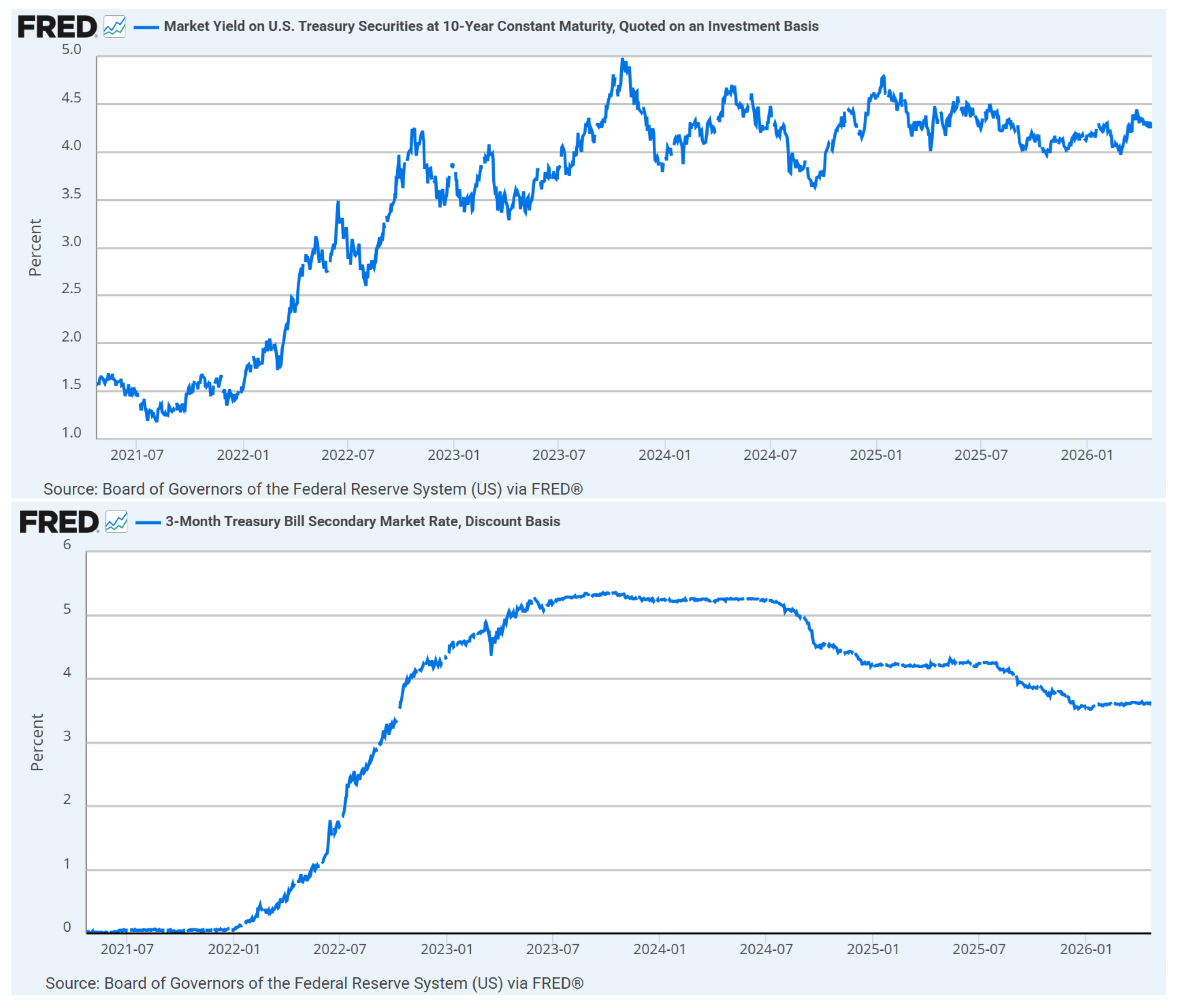
Figure 1 illustrates the evolution of long-term and short-term interest rates over the sample period. The data are obtained from the FRED database and reflect a period of substantial macroeconomic variation.

The 10-year yield exhibits gradual changes over the sample period, while the 3-month yield shows more responsive movement consistent with short-term monetary conditions. The yield spread $s_t$ varies over time and reflects changes in the slope of the yield curve.

These dynamics motivate the use of sequential predictive models that can capture both short-term fluctuations and longer-term temporal dependencies in macro-financial variables. In this study, these features are used as inputs to a supervised learning framework for predicting one-step-ahead yield changes.

3.2. Sequential State Representation

To incorporate temporal dependence, we construct a sequence-based state representation using a rolling window of length $T_{\mathrm{steps}}=5$. Let ${\mathbf{x}}_t\in {\mathbb{R}}^p$ denote the feature vector at time t. The state is defined as

$$S_t=\left({\mathbf{x}}_{t-T_{\mathrm{steps}}+1},\dots ,{\mathbf{x}}_t\right)\in {\mathbb{R}}^{T_{\mathrm{steps}}\times p}.$$

(1)

This representation embeds a short-horizon temporal structure of macro-financial variables into a fixed-dimensional input suitable for supervised learning.

Action Space and Prediction Target

We consider a discrete action space $\mathcal{A}=\{0,1,2\}$ corresponding to hold, up, and down directional predictions on the 10-year Treasury yield.

We define the one-step-ahead target:

$$r_t=y_{t+1}^{\left(10\right)}-y_t^{\left(10\right)}.$$

(2)

The action-dependent realized outcome is defined as

$$Y_t\left(a\right)=\left\{\begin{array}{cc}0,\hfill & a=0,\hfill \\ r_t,\hfill & a=1,\hfill \\ -r_t,\hfill & a=2.\hfill \end{array}\right.$$

(3)

3.3. Empirical Results

Table 1. Performance under Alternative Sampling Strategies.

Model	Mean Outcome	SD Outcome	Final Outcome	Early Outcome	Late Outcome	Improvement
Entropy	−0.000452	0.00188	0.00169	−0.000686	−0.000482	0.000203
Prediction-error (PER)	−0.000116	0.00214	0.000277	−0.00108	−0.000601	0.000479
Uniform	0.000106	0.00169	0.00110	0.000587	0.000480	−0.000108

summarizes the performance of the proposed supervised sequential prediction model under three alternative sampling strategies in a macro-financial environment constructed from Treasury yield curve dynamics.

Overall, the results reveal distinct performance profiles across sampling strategies.

Uniform sampling achieves the highest mean outcome (0.000106) and the lowest variance (0.00169), indicating the most stable predictive performance across heterogeneous macro-financial conditions. This suggests that unbiased sampling provides robustness under nonstationary yield dynamics.

Entropy-based sampling attains the highest final outcome (0.00169), indicating stronger late-stage predictive performance. This reflects the effectiveness of prioritizing regions of high predictive uncertainty and feature dispersion, which enhances learning under complex and noisy dynamics.

Prediction-error-based sampling yields the largest improvement (0.000479) from early to late training stages, indicating faster learning driven by high-residual observations. However, its higher variance suggests reduced robustness under regime shifts.

3.3.1. Macro-Financial Interpretation

The underlying state space is constructed from Treasury yield curve variables, which exhibit pronounced nonstationarity, heteroskedasticity, and regime shifts driven by macroeconomic and monetary policy dynamics. These properties strongly influence sampling effectiveness.

Uniform sampling mitigates regime sensitivity by treating all observations equally, ensuring stable coverage across market conditions. Entropy-based sampling adaptively emphasizes uncertain regions of the feature space, improving robustness under distributional shifts. Prediction-error-based sampling focuses on high-residual observations, accelerating learning but increasing sensitivity to structural changes in the yield curve process.

3.3.2. Overall Findings

The empirical evidence highlights a fundamental trade-off between stability, learning efficiency, and sensitivity to informative but potentially noisy observations. Uniform sampling yields the most stable performance, entropy-based sampling achieves strong late-stage accuracy, and prediction-error-based sampling provides the fastest learning progression.

Importantly, no single sampling strategy dominates across all evaluation criteria. In macro-financial environments characterized by nonstationarity, volatility clustering, and structural breaks, robustness and stability remain as important as learning speed.

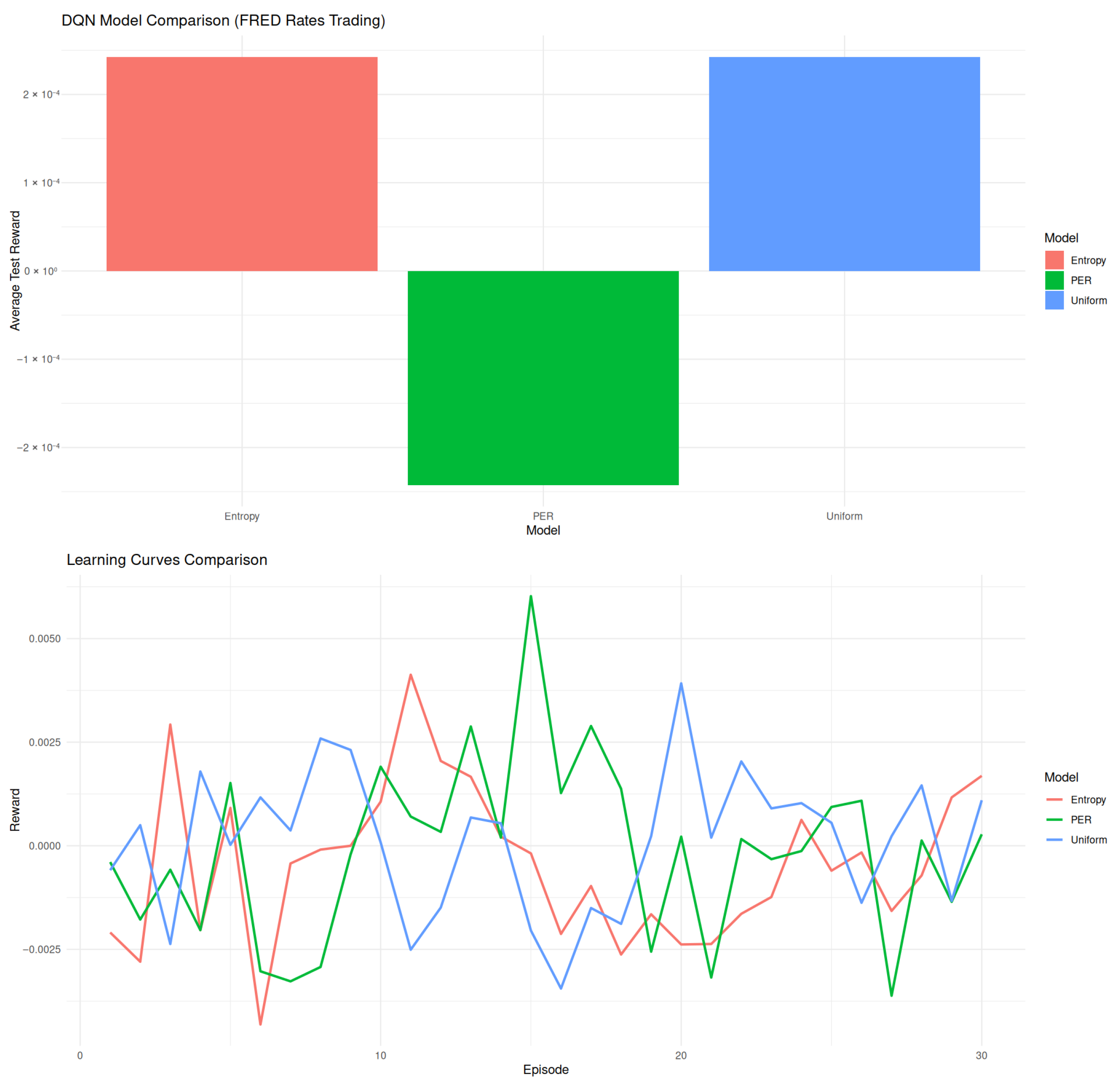
Figure 2 presents an empirical comparison of the proposed supervised sequential prediction model trained on macro-financial variables derived from U.S. Treasury yield curve data obtained from the Federal Reserve Economic Data (FRED) system. The analysis evaluates three sampling strategies within a unified learning framework.

The considered sampling mechanisms are:

• Entropy-based sampling: selects observations using predictive entropy and output dispersion, emphasizing uncertain regions of the feature space.
• Prediction-error-based sampling: prioritizes observations with large prediction residuals.
• Uniform sampling: samples observations uniformly without weighting.

The top panel shows out-of-sample performance measured by average realized outcome. Uniform and entropy-based sampling both achieve small positive test outcomes on the order of ${10}^{-4}$, with uniform sampling performing slightly better. Prediction-error-based sampling yields a marginally negative outcome, indicating weaker generalization in this setting.

The bottom panel shows training dynamics over 30 optimization passes. Uniform and entropy-based sampling produce smoother trajectories, while prediction-error-based sampling exhibits higher volatility due to its emphasis on high-residual observations.

Overall, uniform sampling demonstrates the most stable and robust behavior, entropy-based sampling provides competitive performance with moderate variability, and prediction-error-based sampling accelerates early learning but is less stable under structural changes.

These findings suggest that in macro-financial sequential prediction problems characterized by nonstationarity and regime shifts, simpler sampling mechanisms can be highly competitive, while adaptive strategies require careful calibration to avoid overfitting to noisy or transient observations.

4. Conclusions

This study develops a deep supervised learning framework for macro-financial sequential prediction using U.S. Treasury yield curve dynamics. By constructing a sequence-based state representation from 10-year and 3-month Treasury rates, we model short-horizon movements in interest rates as a predictive learning problem over temporally dependent financial features.

We propose a hybrid convolutional–recurrent neural network that integrates convolutional layers for local temporal pattern extraction and LSTM layers for capturing longer-term dependencies in macroeconomic time series. The model is trained to predict one-step-ahead yield changes under a supervised learning objective.

A key contribution of this work is the introduction of adaptive replay sampling strategies for sequential financial data. We systematically compare uniform sampling, entropy–variance-based sampling, and prediction-error-based sampling. These mechanisms determine how past observations are reused during training and directly influence learning stability and predictive performance.

Empirical results demonstrate that the choice of sampling strategy significantly affects both training dynamics and out-of-sample predictive accuracy. Uniform sampling yields the most stable performance and competitive test outcomes, suggesting robustness under nonstationary macro-financial conditions. Entropy-based sampling achieves strong late-stage performance, indicating the benefit of prioritizing uncertain and information-rich observations. In contrast, prediction-error-based sampling accelerates early learning but exhibits higher variance and reduced stability under structural shifts in interest rate dynamics.

The analysis highlights a fundamental trade-off between stability, convergence behavior, and sensitivity to informative but potentially noisy observations in sequential financial learning problems. In macro-financial environments characterized by nonstationarity, heteroskedasticity, and regime changes, overly aggressive prioritization may reduce robustness unless carefully regularized.

Overall, the results suggest that simple uniform sampling remains highly competitive, while entropy-aware strategies provide a balanced improvement in performance under uncertainty. This study contributes to the literature on deep learning for financial time series by demonstrating that the design of data sampling strategies plays a critical role in sequential predictive modeling under real macro-financial dynamics.