Abstract
The statistical distribution of financial returns plays a key role in evaluating Value-at-Risk using parametric methods. Traditionally, when evaluating parametric Value-at-Risk, the statistical distribution of the financial returns is assumed to be normally distributed. However, though simple to implement, the Normal distribution underestimates the kurtosis and skewness of the observed financial returns. This article focuses on the evaluation of the South African equity markets in a Value-at-Risk framework. Value-at-Risk is estimated on four equity stocks listed on the Johannesburg Stock Exchange, including the FTSE/JSE TOP40 index and the S & P 500 index. The statistical distribution of the financial returns is modelled using the Normal Inverse Gaussian and is compared to the financial returns modelled using the Normal, Skew t-distribution and Student t-distribution. We then estimate Value-at-Risk under the assumption that financial returns follow the Normal Inverse Gaussian, Normal, Skew t-distribution and Student t-distribution and backtesting was performed under each distribution assumption. The results of these distributions are compared and discussed.
1. Introduction
Value-at-Risk (VaR) is defined as the worst expected loss over a given period at a specified confidence level [1]. Jorion [2] describe VaR as the quantile1 of the projected distribution of losses and gains of an investment over a target horizon. VaR answers the question, “How much can I lose with probability over a certain holding period?” [1]. The risk metric VaR, has become a widely used risk measure by financial institutions and regulatory authorities2, as it attempts to provide a single number that summarizes the overall market risk in individual stocks and for portfolios [4].
VaR is a tool used to measure market risk, where market risk is the potential for change in the value of an investment due to change in market risk factors [1]. Market risk factors are interest rates, commodity prices, foreign exchange rates and stock and bond prices [1]. Historically, market risk was measured by the standard deviation of unexpected outcomes or by simple indicators of the notional-amount of the individual stock [5]. McNeil et al., in [5], provide the pros and cons of each traditional measures of market risk.
When evaluating VaR for financial assets the distribution of the returns of the underlying asset play an important role. Methodology of estimating VaR can be classified into two groups, i.e., the parametric VaR and non-parametric VaR. The classification of VaR methodology is based on how the financial return distribution is modelled. Parametric VaR assumes that financial returns are modelled using a statistical distribution (e.g., Normal and Student t-distribution). Whereas non-parametric VaR assumes that financial returns are modelled using the empirical distribution. The statistical distribution that is commonly assumed in parametric VaR is the Normal distribution, which is easy to implement as it depends on two parameters, i.e., the mean and standard deviation of historical returns. However, a number of studies have shown that daily financial returns are non-normal, they display a leptokurtic and skewed distribution as noted by Mandelbrot [6] and Fama [7]. A leptokurtic distribution has a higher peak and heavier tails than the Normal distribution [8]. In other words, the frequency of financial returns near the mean will be higher and extreme movements are more likely than the Normal distribution would predict. For example, if we consider South African FTSE/JSE TOP40 Index the largest decrease was roughly , which occurred in 1997. The decrease deviates by ten standard deviations from the mean and by modelling financial returns with the Normal distribution this decrease is practically impossible.
The quality of VaR is dependent on how well the statistical distribution captures the leptokurtic behaviour of the financial returns [9]. Shortcoming of statistical distribution can result in incorrect estimation of risk and lead to serious mismanagement of risk, for example insufficient capital invested to limit the probability of extreme losses. Hence, finding a statistical distribution that represents the leptokurtic behaviour of financial returns in VaR estimation remains an important research topic. The introduction of VaR as the market risk measure has seen a number of empirical studies being done to find alternative distributions to the Normal distribution. These studies include application of the Student t-distribution (t-distribution in VaR estimation for returns on US equities and bonds by Huisman, Koedijk, and Pownall [10]. Application of the t-distribution in VaR estimation within the South African equity market was done by Milwidsky and Maré [11]. The t-distribution is also used by McNeil and Frey in [12] and Platen and Rendek [13]. Although the t-distribution addresses the issue of heavy tails, it fails to address the skewness present in financial returns because it is symmetrical about zero. The lack of skewness in the t-distribution was first addressed by Hansen in [14], when he first proposed a skew extension to the t-distribution for modelling financial returns. Since then, several authors have studied the application of the Skew Student t-distribution (Skew t) to modelling financial returns, see for example, Azzalini and Capitanio [15], Aas and Haff [16], Jones and Faddy [17]. The other proposed distribution is the Extreme Value Theory, which only models the behaviour of losses and not the entire returns distribution. For application of the Extreme Value Theory refer to: Longin [18], Danielsson and De Vries [19], McNeil and Frey [12], Embrechts, Klüppelberg and Mikosch [20], Gençay, Selçuk, and Ulugülyağci [21] and Wentzel and Maré [22]. Other methods used include, modelling the returns and volatility process by the ARMA (1,1)-GARCH (1,1) time series and then fitting the residuals with the selected distribution, which this article will not be pursing, see for example Bhattachariya and Madhav [23], Schaumburg [24] and Kuester et al. [25].
The focal point of this article is to apply the NIG distribution to the evaluation of the South African equity markets in a Value-at-Risk framework. This study is based on the work of Bølviken and Benth [26], who investigated the NIG distribution as a tool to evaluate the uncertainty in future prices of the shares listed on the Norwegian Stock Exchange in Oslo. At the time of writing this article, we became aware of the work on VaR by Huang et al. [27]. In their work, they utilized the NIG, Skew t and Generalised Hyperbolic for modelling the South African Mining Index returns. The NIG distribution is able to capture the skewness and kurtosis present in the financial returns. The tails of the NIG distribution are described as “semi-heavy”. Dependent on four parameters that affect the shape of the density function, with the NIG distribution one is able to create different shapes of the density function by adjusting the parameters, making the NIG distribution very flexible. Most of the authors have report an excellent fit to the financial returns. Application and reviews of the NIG distribution is given by Lillestøl [28], Rydberg [9], Prause [29], Barndorff-Nielsen [30], Venter and de Jongh [31] and Bølviken and Benth [26]. The NIG distribution has an important property of being closed under convolution i.e., the sum of independent NIG random variables is also NIG distributed. This property is useful when working with a portfolio of shares and for time scaling of VaR.
The goal of the article is to implement the NIG distribution and compare the fitting to that of the Skew t, t-distribution and Normal distribution over four sample periods defined in Section 2. Lastly, we estimate Value-at-Risk under the NIG assumption and compare the numbers to those under the Normal, t-distribution, Skew t and the Extreme Value Theory. This study is restricted to market risk associated with price changes of equity stocks listed on the Johannesburg Stock Exchange in South Africa over 1-day time horizon. Therefore, VaR is estimated in linear positions in the underlying equity stocks. In Section 2 we give a summary of the listed companies and indices that we will be using to evaluate Value-at-Risk. In Section 3 we fit the NIG, Skew t, t-distribution and Normal distribution to the chosen stocks and indices and compare the fit using the Kolmogorov-Smirnov distance between the empirical distribution and the fitted distribution. In Section 4 we evaluate Value-at-Risk and ES for the chosen equity stocks and indices assuming that the underlying distribution is NIG, t-distribution and Skew t and conclude the section with the backtesting results. Finally, in Section 5 we discuss our findings and draw some conclusions. The graphs and some of the tables are presented in the last five pages of this article.
2. Empirical Study
In this section, we consider the listed equity data and give a brief insight into our data.
2.1. Empirical Data
The empirical study is done using four South African equity stocks, FTSE/JSE TOP40 (J200) index and the S & P 500 index. The four shares (Standard Bank (SBK), African Bank (ABL), Merafe Resource (MRF) and Anglo American (AGL)) are listed on the Johannesburg Stock Exchange. Maximum available daily closing prices for the equity stocks were obtained resulting in varying periods ending 31 July 2014. The S & P 500 data is from 2 January 1991 to 28 March 2014, totalling 5831 daily returns, while the FTSE/JSE TOP40 index data is from 30 June 1995 to 31 July 2014. These equity stocks were randomly selected and they reflect different but not the entire sub-sectors of the JSE main board. Standard Bank and Anglo American have large market capitalization and we expect them to mimic the FTSE/JSE TOP40, while Merafe and African Bank are small and therefore would have an element of jump risk.
- Merafe Resources is listed on the JSE under the General Mining sector. Merafe mines chrome, which they use to produce ferrochrome. The historical daily closing prices used for our analysis was for the period from 17 December 1999 to 1 July 2013.
- Standard Bank is listed under the Banking sector. The company provides services in personal, corporate, merchant and commercial banking, mutual fund and property fund management among other services. The daily closing prices used for analysis Standard Bank data was over the period 1 September 1997 to 31 July 2014.
- African Bank is listed under Consumer Finance. The bank provides unsecured credit, retail and financial services. We use daily closing prices over the period 29 September 1997 to 31 July 2014.
- Anglo American is listed under the General Mining sector and they mine platinum, diamonds, iron ore and thermal coal. The daily closing prices over the period from 1 September 1999 to 31 July 2014 were used.
We included the FTSE/JSE TOP40 index, which consists of the 40 largest companies listed on the JSE in terms of market capitalization. The Index gives reasonable reflection of the entire South African stock market as these 40 top companies represent over 80% of the total market capitalization of all the companies listed on the JSE [32]. The daily log returns defined by were obtained totalling a series of observations for South African listed shares, where N is the total number of closing prices observed for each share and is the closing price/index level at day t. We assume the share prices and index level to follow a random walk and exclude dividends.
The sample period has been split into three sub-samples, that is:
- Pre-crisis (from 1991 January–December 2007),
- Crisis period (from January 2008–December 2009),
- Post-crisis (from January 2010–July 2014).

Table 1.
Statistical data for each stock and indices.
| Statistical Data of the Empirical Distribution over the Period January 1991–July 2014. | |||||
| Mean | Variance | Skewness | Excess Kurtosis | No. OBS3 | |
| S & P 500 | 6170 | ||||
| FTSE/JSE TOP40 | 4770 | ||||
| Standard Bank | 4090 | ||||
| African Bank | 3944 | ||||
| Anglo American | 4162 | ||||
| Merafe Resource | 2806 | ||||
| Pre-Crisis (from January 1991–December 2007) Statistical Data. | |||||
| Mean | Variance | Skewness | Kurtosis | No. OBS | |
| S & P 500 | 0.0004 | 0.0001 | –0.0746 | 3.8997 | 4262 |
| FTSE/JSE TOP40 | 0.0006 | 0.0002 | –0.6571 | 8.1379 | 3124 |
| Standard Bank | 0.0006 | 0.0006 | –0.3163 | 4.9000 | 2463 |
| African Bank | 0.0007 | 0.0009 | –0.4599 | 7.9791 | 2338 |
| Anglo American | 0.0008 | 0.0006 | –0.0394 | 3.0429 | 2520 |
| Merafe Resources | 0.0014 | 0.0014 | 0.4452 | 1.3903 | 1485 |
| Crisis Period (from January 2008–December 2009) Statistical Data. | |||||
| Mean | Variance | Skewness | Kurtosis | No. OBS | |
| S & P 500 | –0.0005 | 0.0005 | –0.0963 | 4.3544 | 505 |
| FTSE/JSE TOP40 | –0.0001 | 0.0005 | 0.0408 | 1.3969 | 501 |
| Standard Bank | 0.0000 | 0.0007 | 0.1997 | 1.3906 | 490 |
| African Bank | –0.0002 | 0.0009 | 0.0418 | 0.4575 | 491 |
| Anglo American | –0.0005 | 0.0016 | –0.1295 | 1.8202 | 499 |
| Merafe Resources | –0.0011 | 0.0022 | –0.6017 | 2.7368 | 457 |
| Post-Crisis (from January 2010–July 2014) Statistical Data. | |||||
| Mean | Variance | Skewness | Kurtosis | No. OBS | |
| S & P 500 | 0.0004 | 0.0001 | –3.2713 | 49.1255 | 1403 |
| FTSE/JSE TOP40 | 0.0005 | 0.0001 | –0.1593 | 1.3757 | 1145 |
| Standard Bank | 0.0003 | 0.0002 | –0.1336 | 1.1070 | 1137 |
| African Bank | –0.0014 | 0.0006 | –2.5109 | 29.7154 | 1115 |
| Anglo American | –0.0001 | 0.0003 | 0.1624 | 0.5933 | 1143 |
| Merafe Resources | –0.0000 | 0.0008 | 0.1183 | 1.8172 | 864 |
Most of the analysis is performed using the entire sample period and the three sub-samples. We start off with a statistical summary of the data for each share and the indices over varying periods ending 31 July 2014. Table 1 above shows the statistical summary of the data for each share, computed using the daily log returns. Based on the statistical results of the empirical data in Table 1 the mean of the each stock and the index is relatively small; compared to the variance it is almost insignificant. The excess kurtosis for each stock and the index is greater than zero. This indicates a higher peak and heavier tails meaning extreme loss and profit are more likely to occur than what the Normal distributed would predict.
The Indices, Standard Bank, African Bank and Anglo American have negative skewness that is the left tail is longer, indicating that losses occur more frequently than profits over the entire sample period. While Merafe has positive skewness implying more profits than losses were realised over the period. In general each stock and the indices display fatter tails and skewness in comparison to the Normal distribution as noted in literature [7].
3. Fitting the Distribution
3.1. Normal Inverse Gaussian Distribution
The NIG distribution is a special case of the generalised hyperbolic distributions introduced by Barndorff-Nielsen in 1977 [30]. It is a continuous distribution defined on the entire real line.
Definition 1. [33] The random variable X follows a NIG distribution with parameters α, β, μ and δ, if its probability density function, defined for all real , is given by:
where the function is a modified Bessel function of third order and index 1. In addition the parameters must satisfy , , and . If a random variable x follows a NIG distribution it can be denoted in short as .
The NIG distribution is characterized by four parameters and δ, each relating to the overall shape of the density distribution. These parameters are usually categorized in one of the two groups. The first group of parameters affecting the scaling and location of the distribution are μ and δ. The second group of parameters affecting the shape of the distribution are α and β.
The parameter α measures the tail heaviness of the distribution, the larger α the thinner the tails and the smaller α the fatter the tails. The skewness of NIG distribution is measured by β. When , the distribution is symmetric around μ. If , then the distribution is skewed to the right, whereas negative β gives skewness to the left [26]. The parameter μ and δ have the same interpretation as the mean and standard deviation on the Normal distribution. The parameter μ describes the location of the peak of the distribution or were the distribution is centered on the real number line [26], while δ describes the spread of the returns.
One of the important properties of the NIG distribution is that it is closed under convolution. This means, the sum of independent and identical random variables which are NIG distributed is also NIG distributed. The NIG distribution has semi-heavy tail. In particular by using the following asymptotic formula of the Bessel function:
Barndorff-Nielsen [30] found that the tail of the NIG behaves as:
for , where and the constant A is given by:
This means, the tails of the NIG distribution are always heavier than those of the Normal distribution. In addition, a clever selection of parameters can create a wide range of density shapes, making the NIG distribution a very flexible tool to use for modelling financial returns.
3.2. The Student’s t-Distribution
The t-distribution suggested by Blattberg and Gonedes [34] as an alternative distribution to model financial returns, it is characterized by the shape-defining parameter known as the degree of freedom . The density function is given by:
where x is the random variable, k is the degree of freedom and Γ is the gamma function. The t-distribution is similar to Normal distribution, it is symmetrically about the mean except it exhibit fatter tails. The variance is given by . The degree of freedom k controls the fat tails of the distribution, the smaller the value of k the fatter the tails of the distribution. When k increases the variance approaches 1 and therefore the t-distribution converges the Normal distribution.
3.3. The Skew t-Distribution
The Skew t is the skew extension of the t-distribution. It was first proposed by Hansen in [14] as an alternative distribution to model financial returns. There are several definitions of the density function of the Skew t given in literature. We apply the one proposed by Azzalini and Capitanio in [15] and it is given by
where is the density function of the t-distribution given in Equation (2) with degrees of freedom k and β is the skewness parameter. When , the Equation (3) reduces to the t-distribution. The Skew t has heavy tails, which mean that it should model data with heavy tails well but may not handle extensive skewness [16].
We fit the NIG model to the empirical data described in Section 2 and compare the fit of the NIG to the fit of the Skew t, Normal and t-distribution. Fitting the NIG distribution is straightforward using the statistical program R with the package fBasics [35] because the program has a predefined function for the maximum likelihood estimation (MLE) of the NIG distribution. Table 2 shows the maximum likelihood parameter estimates results for the fitted distributions and the graphical representation of the parameters is presented in Figure 1, where for example alpha, beta, delta and mu are the NIG parameter estimates of the entire sample period and alpha1, beta1, delta1 and mu1 represent the NIG parameter estimates of the Pre-crisis period.
Table 2.
Maximum likelihood parameter estimates.
| Parameter Estimates over the Period January 1991–July 2014 | |||||||
| NIG | t-Dist. | Skew t | |||||
| S & P 500 | 58.3541 | –5.0934 | 0.0075 | 0.0009 | 2.7962 | 2.8038 | 0.9519 |
| FTSE/JSE TOP 40 | 67.8875 | –5.109 | 0.0123 | 0.0014 | 4.0000 | 3.8419 | 0.9533 |
| Standard Bank | 44.7345 | 0.3524 | 0.0208 | 0.0003 | 4.0000 | 4.0006 | 1.0145 |
| African Bank | 32.372 | –0.6613 | 0.025 | 0.0005 | 3.8414 | 4.0000 | 1.0000 |
| Anglo American | 43.1323 | 0.9557 | 0.027 | –0.0002 | 4.6143 | 4.6127 | 1.0208 |
| Merafe Resources | 41.3981 | 4.5965 | 0.0527 | –0.0054 | 6.5225 | 6.2649 | 1.1460 |
| Pre-crisis (from January 1991–December 2007) Parameter Estimates | |||||||
| NIG | t-Dist. | Skew t | |||||
| S & P 500 | 82.3073 | –2.7308 | 0.0084 | 0.0006 | 4.0000 | 3.5163 | 0.9765 |
| FTSE/JSE TOP40 | 77.3477 | –5.8151 | 0.0128 | 0.0015 | 4.0000 | 4.2290 | 0.9605 |
| Standard Bank | 44.1135 | –0.1645 | 0.0238 | 0.0007 | 4.0000 | 4.3920 | 1.0121 |
| African Bank | 32.4499 | 0.9420 | 0.0274 | –0.0001 | 4.0105 | 4.0001 | 1.0373 |
| Anglo American | 53.2541 | 0.9913 | 0.0306 | 0.0002 | 5.6917 | 5.6988 | 1.0134 |
| Merafe Resources | 58.7370 | 15.7660 | 0.0737 | –0.0192 | 9.2786 | 9.2746 | 1.2459 |
| Crisis Period (from January 2008–December 2009) Parameter Estimates | |||||||
| NIG | t-Dist. | Skew t | |||||
| S & P 500 | 27.9336 | –3.9019 | 0.0137 | 0.0014 | 2.5545 | 2.5254 | 0.9124 |
| FTSE/JSE TOP40 | 59.4900 | –0.3225 | 0.0270 | 0.0000 | 5.7367 | 5.7149 | 0.9874 |
| Standard Bank | 45.3549 | 4.4290 | 0.0323 | –0.0031 | 5.5645 | 5.6319 | 1.0618 |
| African Bank | 78.1936 | 5.9075 | 0.0715 | –0.0056 | 14.7400 | 14.4505 | 1.0546 |
| Anglo American | 29.5059 | –0.0252 | 0.0474 | –0.0005 | 5.2692 | 5.2457 | 1.0149 |
| Merafe Resources | 29.4521 | –4.0030 | 0.0611 | 0.0073 | 5.6407 | 5.8777 | 0.9300 |
| Post-Crisis (from January 2010–July 2014) Parameter Estimates | |||||||
| NIG | t-Dist. | Skew t | |||||
| S & P 500 | 70.5049 | –13.0538 | 0.0070 | 0.0017 | 2.9116 | 2.9563 | 0.9094 |
| FTSE/JSE TOP40 | 122.4542 | –13.7630 | 0.0132 | 0.0020 | 5.6707 | 5.7635 | 0.9264 |
| Standard Bank | 128.9099 | –7.2170 | 0.0251 | 0.0017 | 8.8356 | 4.0000 | 1.0000 |
| African Bank | 34.4911 | –7.7071 | 0.0175 | 0.0026 | 3.3022 | 3.3084 | 0.8747 |
| Anglo American | 123.3751 | 11.4136 | 0.0420 | –0.0040 | 12.8391 | 13.2898 | 1.0454 |
| Merafe Resources | 72.0322 | 11.2690 | 0.0558 | -0.0088 | 10.1389 | 8.8798 | 1.2196 |

Figure 1.
Graphical representation of the NIG, t-distribution and Skew t-distribution maximum likelihood parameters estimates.
Figure 1.
Graphical representation of the NIG, t-distribution and Skew t-distribution maximum likelihood parameters estimates.
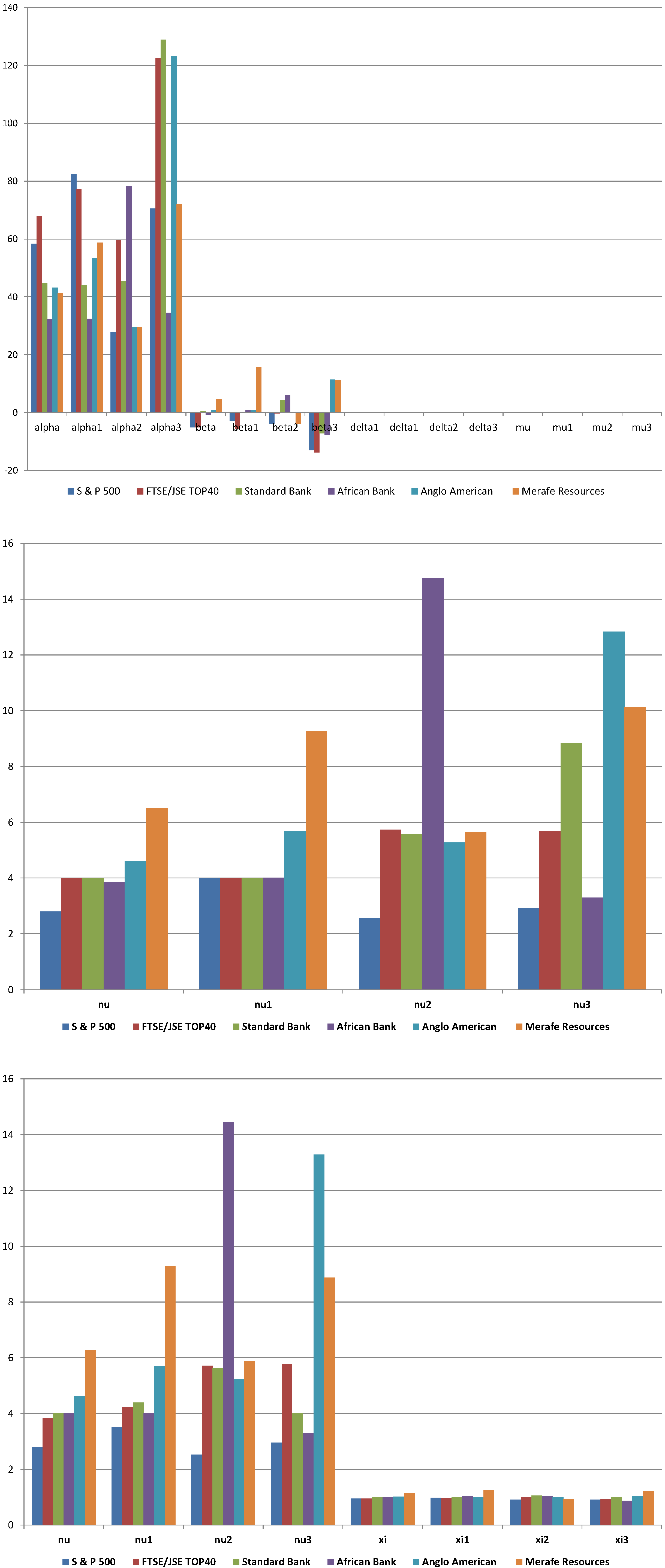
Table 3.
Kolmogorov-Smirnov test statistics and estimated critical values for the fitted distributions.
| Parameter Estimates for the Period January 1991–July 2014 | ||||||||
| Kolmogorov-Smirnov | Critical Value | |||||||
| NIG | t-Dist. | Skew t | Normal | |||||
| S & P 500 | 0.0058 | 0.0135 | 0.0113 | 0.0875 | 0.0156 | 0.0173 | 0.0188 | 0.0207 |
| FTSE/JSE TOP40 | 0.0081 | 0.0082 | 0.0046 | 0.0580 | 0.0177 | 0.0197 | 0.0214 | 0.0236 |
| Standard Bank | 0.0201 | 0.0190 | 0.0184 | 0.0560 | 0.0191 | 0.0212 | 0.0231 | 0.0255 |
| African Bank | 0.0173 | 0.0150 | 0.0149 | 0.0657 | 0.0195 | 0.0216 | 0.0236 | 0.0259 |
| Anglo American | 0.0114 | 0.0101 | 0.0088 | 0.0443 | 0.0190 | 0.0211 | 0.0229 | 0.0252 |
| Merafe Resources | 0.0809 | 0.0862 | 0.0828 | 0.0765 | 0.0232 | 0.0257 | 0.0280 | 0.0308 |
| Pre-Crisis (from January 1991–December 2007) Parameter Estimates | ||||||||
| Kolmogorov-Smirnov | Critical Value | |||||||
| NIG | t-Dist. | Skew t | Normal | |||||
| S & P 500 | 0.0117 | 0.0187 | 0.0163 | 0.0626 | 0.0187 | 0.0208 | 0.0227 | 0.0249 |
| FTSE/JSE TOP40 | 0.0116 | 0.0103 | 0.0092 | 0.0535 | 0.0219 | 0.0243 | 0.0265 | 0.0291 |
| Standard Bank | 0.1934 | 0.0288 | 0.0272 | 0.0546 | 0.0247 | 0.0274 | 0.0298 | 0.0328 |
| African Bank | 0.0245 | 0.0247 | 0.0224 | 0.0641 | 0.0253 | 0.0281 | 0.0306 | 0.0337 |
| Anglo American | 0.0112 | 0.0104 | 0.0105 | 0.0349 | 0.0244 | 0.0271 | 0.0295 | 0.0324 |
| Merafe Resources | 0.0885 | 0.0994 | 0.0968 | 0.0982 | 0.0318 | 0.0352 | 0.0384 | 0.0422 |
| Crisis Period (from January 2008–December 2009) Parameter Estimates | ||||||||
| Kolmogorov-Smirnov | Critical Value | |||||||
| NIG | t-Dist. | Skew t | Normal | |||||
| S & P 500 | 0.0278 | 0.0369 | 0.0288 | 0.0860 | 0.0545 | 0.0604 | 0.0659 | 0.0724 |
| FTSE/JSE TOP40 | 0.0162 | 0.0177 | 0.0181 | 0.0410 | 0.0547 | 0.0607 | 0.0661 | 0.0727 |
| Standard Bank | 0.0235 | 0.0285 | 0.0287 | 0.0618 | 0.0553 | 0.0614 | 0.0669 | 0.0735 |
| African Bank | 0.0261 | 0.0297 | 0.0237 | 0.0279 | 0.0552 | 0.0613 | 0.0668 | 0.0735 |
| Anglo American | 0.0322 | 0.0342 | 0.0336 | 0.0676 | 0.0548 | 0.0608 | 0.0663 | 0.0729 |
| Merafe Resources | 0.0596 | 0.0557 | 0.0606 | 0.0594 | 0.0573 | 0.0635 | 0.0692 | 0.0761 |
| Post-Crisis (from January 2010–July 2014) Parameter Estimates | ||||||||
| Kolmogorov-Smirnov | Critical Value | |||||||
| NIG | t-Dist. | Skew t | Normal | |||||
| S & P 500 | 0.0160 | 0.0212 | 0.0165 | 0.1066 | 0.0327 | 0.0363 | 0.0395 | 0.0435 |
| FTSE/JSE TOP40 | 0.0135 | 0.0166 | 0.0171 | 0.0504 | 0.0362 | 0.0401 | 0.0437 | 0.0481 |
| Standard Bank | 0.0175 | 0.0160 | 0.0254 | 0.0293 | 0.0363 | 0.0403 | 0.0439 | 0.0483 |
| African Bank | 0.0279 | 0.0236 | 0.0152 | 0.0942 | 0.0367 | 0.0407 | 0.0443 | 0.0487 |
| Anglo American | 0.0150 | 0.0138 | 0.0142 | 0.0266 | 0.0362 | 0.0402 | 0.0438 | 0.0481 |
| Merafe Resources | 0.0945 | 0.0932 | 0.1072 | 0.0899 | 0.0416 | 0.0462 | 0.0504 | 0.0554 |
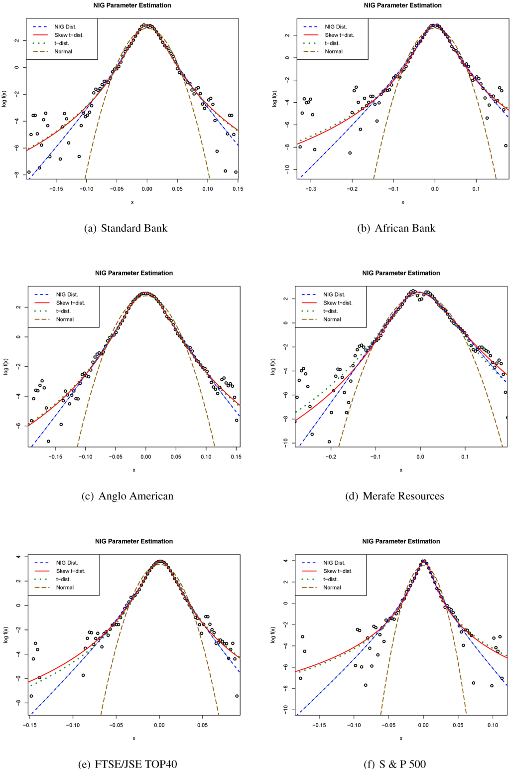
Figure 2.
The log-density of the empirical data with the fitted NIG, Normal, Skew t and t-distribution.
Figure 2.
The log-density of the empirical data with the fitted NIG, Normal, Skew t and t-distribution.
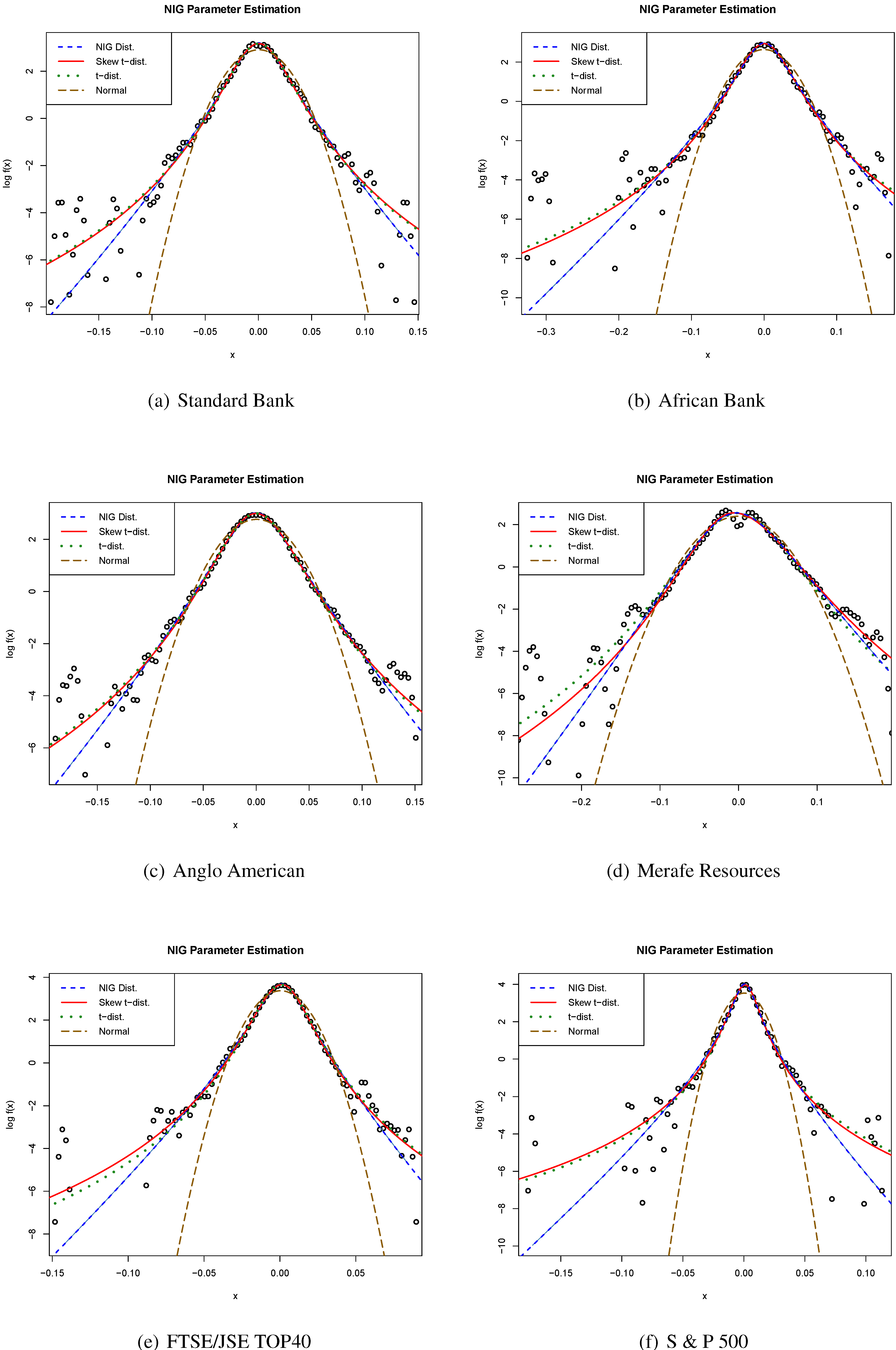
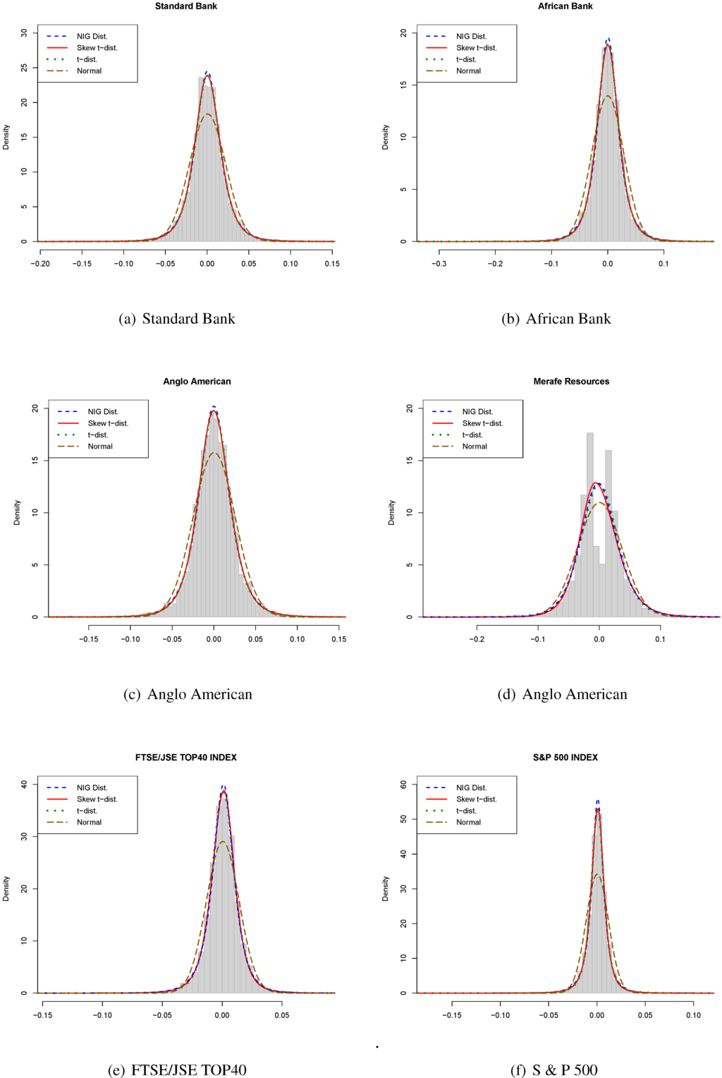
Figure 3.
Comparison of each stock and the indices histograms with the fitted NIG, Skew t, t-distribution and Normal distribution.
Figure 3.
Comparison of each stock and the indices histograms with the fitted NIG, Skew t, t-distribution and Normal distribution.

Table 3 shows the Kolmogorov-Smirnov test statistic values and critical values for different confidence levels. The test statistic values are the distance between the empirical cumulative distribution and the fitted cumulative distribution. The results of the table shows that we do not reject the null hypothesis for the NIG, Skew t and t-distribution. However, the null hypothesis is rejected for the Normal distribution for all the shares with exception of Merafe Resources and in some cases the other three distributions are rejected for Merafe Resources as well. Figure 2 compares the log-density of the NIG, Normal, Skew t and t-distribution to the empirical data, the overall observation is that the Skew t and t-distribution have fatter tailed compared to the NIG distribution. In addition, the NIG, Skew t and t-distribution seem to adequately fit the center of the empirical distribution quite well compared to the Normal distribution. The Normal distribution has a shape of a parabola and deviates from the tails of the empirical log-density.
From Figure 3, it is observed that the NIG, Skew t and t-distribution fits the empirical histogram better than that of the Normal distribution. These three distributions also match the empirical distribution better with respect to the skewness and the peak compared to the Normal distribution, while the NIG show a slightly higher peak.
4. Value-at-Risk
In this section we present the comparison of Value-at-Risk estimates under the NIG, Skew t, Normal and t-distribution to the empirical distribution of the stocks and indices. We further verify the correctness of the VaR models using the backtesting technique.
4.1. Value-at-Risk Estimates
The VaR and ES estimates obtained under the NIG, Skew t, Normal and t-distribution assumption for a one-day holding period at confidence level are shown in Table 4 and Table 5, respectively. The VaR and ES estimates under the NIG, Normal, Skew t and t-distribution assumption were calculated using the Monte Carlo simulation. The results for these two tables shows that the VaR estimates under the Normal distribution underestimates the VaR and ES values, as it is well known in literature. The VaR estimates under the NIG, Skew t and t-distribution better values when compared to the Historical VaR and ES values.
4.2. Backtesting the Model
To verify the correctness of the VaR models we perform backtesting method. This is to check how often the daily losses exceed the daily VaR estimate. The number of daily losses exceeding VaR estimate are referred to as violations. The verification of the VaR model’s accuracy is fundamental to the Basel Committee so as to prevent financial institutions understating their risk and the framework of backtesting is set out in [36]. The regulatory backtesting procedure is performed over the last 250 trading days with the one-day VaR compared to the observed daily profits and losses over the period. For example, over 250 trading days, a daily VaR model should have on average violations out of 250. The backtesting results are classified into three zones which are green, yellow and red zones, these zones are linked to the capital requirement scaling factor. See Table 6.
Table 4.
Comparison of the Value-at-Risk estimates, the non-parametric estimates are calculated using the Historical Simulation approach.
| VaR Estimates over the Period January 1991–July 2014 | |||||
| Historical | NIG | t-Dist. | Skew t | Normal | |
| S & P 500 | 3.15% | 3.31% | 3.04% | 3.45% | 2.68% |
| FTSE/JSE TOP 40 | 3.79% | 3.75% | 3.56% | 3.84% | 3.11% |
| Standard Bank | 5.81% | 5.81% | 5.65% | 5.86% | 4.87% |
| African Bank | 7.35% | 7.53% | 7.73% | 7.54% | 6.37% |
| Anglo American | 6.60% | 6.38% | 6.73% | 6.46% | 5.97% |
| Merafe Resources | 9.02% | 8.98% | 9.36% | 8.13% | 8.36% |
| Pre-Crisis (from January 1991–December 2007) VaR Estimates | |||||
| Historical | NIG | t-Dist. | Skew t | Normal | |
| S & P 500 | 2.6213% | 2.8307% | 2.5053% | 2.8592% | 2.3426% |
| FTSE/JSE TOP40 | 3.7136% | 3.5412% | 3.5011% | 3.6038% | 2.9309% |
| Standard Bank | 6.4264% | 6.1871% | 6.0822% | 6.2585% | 5.2607% |
| African Bank | 7.6811% | 8.2170% | 7.9237% | 7.7267% | 7.0160% |
| Anglo American | 6.1856% | 6.2482% | 6.0138% | 5.9658% | 5.5577% |
| Merafe Resources | 8.0043% | 8.3464% | 9.2559% | 7.9108% | 8.3902% |
| Crisis Period (from January 2008–December 2009) VaR Estimates | |||||
| Historical | NIG | t-Dist. | Skew t | Normal | |
| S & P 500 | 6.2799% | 7.2567% | 6.3789% | 8.4283% | 5.1633% |
| FTSE/JSE TOP40 | 5.3725% | 5.6579% | 5.4216% | 5.5736% | 4.8682% |
| Standard Bank | 6.5636% | 6.6214% | 6.9057% | 6.3490% | 6.1787% |
| African Bank | 6.8522% | 7.2559% | 7.6928% | 7.2836% | 6.9659% |
| Anglo American | 9.9742% | 10.5935% | 10.9597% | 10.1201% | 9.4863% |
| Merafe Resources | 13.5510% | 12.4084% | 11.6611% | 12.8104% | 10.9410% |
| Post-Crisis (from January 2010–July 2014) VaR Estimates | |||||
| Historical | NIG | t-Dist. | Skew t | Normal | |
| S & P 500 | 2.8858% | 2.8198% | 2.9767% | 3.2944% | 2.5355% |
| FTSE/JSE TOP40 | 2.8897% | 2.7751% | 2.8675% | 2.8675% | 2.3807% |
| Standard Bank | 3.6093% | 3.6265% | 3.3549% | 4.1969% | 3.1541% |
| African Bank | 6.8760% | 7.7128% | 6.5781% | 7.1226% | 6.1529% |
| Anglo American | 4.3435% | 4.4079% | 4.5477% | 4.4322% | 4.2903% |
| Merafe Resources | 6.4198% | 6.6560% | 7.0918% | 6.3123% | 6.3751% |
Table 5.
Comparison of the one-day Expected Shortfall estimates. The non-parametric estimates are calculated using the Historical Simulation approach.
| Estimates of One-Day Expected Shortfall. | |||||
| Historical | NIG | t-Dist. | Skew t | Normal | |
| FTSE/JSE TOP 40 | |||||
| S & P 500 | |||||
| Standard Bank | |||||
| African Bank | |||||
| Anglo American | |||||
| Merafe Resources | |||||
| Pre-crisis (from January 1991–December 2007) Expected Shortfall Estimates. | |||||
| Historical | NIG | t-Dist. | Skew t | Normal | |
| S & P 500 | 3.47% | 3.64% | 3.39% | 4.19% | 2.67% |
| FTSE/JSE TOP40 | 5.21% | 4.57% | 4.85% | 4.94% | 3.39% |
| Standard Bank | 8.76% | 7.99% | 8.20% | 8.25% | 5.99% |
| African Bank | 11.35% | 10.28% | 11.17% | 10.22% | 8.01% |
| Anglo American | 7.96% | 7.79% | 8.04% | 7.44% | 6.35% |
| Merafe Resources | 9.77% | 10.01% | 11.37% | 9.51% | 9.67% |
| Crisis Period (from January 2008–December 2009) Expected Shortfall Estimates. | |||||
| Historical | NIG | t-Dist. | Skew t | Normal | |
| S & P 500 | 8.20% | 9.49% | 11.42% | 21.09% | 5.88% |
| FTSE/JSE TOP40 | 6.58% | 6.80% | 7.06% | 7.26% | 5.49% |
| Standard Bank | 7.96% | 8.20% | 8.94% | 8.20% | 7.11% |
| African Bank | 8.86% | 8.47% | 8.99% | 8.51% | 7.95% |
| Anglo American | 14.01% | 13.35% | 14.02% | 13.44% | 10.78% |
| Merafe Resources | 17.44% | 15.43% | 14.84% | 16.01% | 12.50% |
| Post-Crisis (from January 2010–July 2014) Expected Shortfall Estimates. | |||||
| Historical | NIG | t-Dist. | Skew t | Normal | |
| S & P 500 | 4.74% | 3.91% | 4.72% | 5.17% | 2.90% |
| FTSE/JSE TOP40 | 3.29% | 3.69% | 3.62% | 3.69% | 2.71% |
| Standard Bank | 4.37% | 4.37% | 4.06% | 6.01% | 3.64% |
| African Bank | 12.55% | 10.28% | 9.82% | 10.50% | 7.06% |
| Anglo American | 4.95% | 5.08% | 5.53% | 5.13% | 4.93% |
| Merafe Resources | 9.10% | 8.00% | 8.61% | 7.78% | 7.43% |
We compare the VaR estimates obtained on the 31 July 2014 to the actual observed returns over the period 1 August 2013 to 31 July 2014, the results are presented in Table 7. We record the number of times the VaR estimates on 31 July 2014 exceeds the observed returns over the period 1 August 2013 to 31 July 2014 and classified the results into the three zones defined by the Basel Committee. For example, the results in Table 7 show that African Bank is the only stock that had a higher number of exceptions with the VaR estimates for NIG, Skew t and t-distribution recording 6 violations. Under the same example the VaR estimate for the Normal distribution recorded 11 violations.
Table 6.
The Basel Committee [36] classification of backtesting outcomes with corresponding number of violations and their scaling factor.
| Zone | Number of Violations | Scaling Violations |
|---|---|---|
| Green | 0 to 4 | 3 |
| Yellow | 5 | |
| 6 | ||
| 7 | ||
| 8 | ||
| 9 | ||
| Red | 10 or more | 4 |
Table 7.
Backtesting results for one-day VaR at 99% a confidence level over the most recent 250 days of our data.
| Backtesting Results for 99% Daily-VaR over the Most Recent 250 Days of Our Data. | ||||||
|---|---|---|---|---|---|---|
| Historical | NIG | Skew t | t-Dist. | Normal | ||
| Standard Bank | No. of ex | 0 | 0 | 0 | 0 | 0 |
| Zone | Green | Green | Green | Green | Green | |
| African Bank | No. of ex | 6 | 6 | 6 | 6 | 11 |
| Zone | Yellow | Yellow | Yellow | Yellow | Red | |
| Anglo American | No. of ex | 0 | 0 | 0 | 0 | 0 |
| Zone | Green | Green | Green | Green | Green | |
| Merafe Resource | No. of ex | 0 | 0 | 0 | 0 | 0 |
| Zone | Green | Green | Green | Green | Green | |
| FTSE/JSE Top40 | No. of ex | 0 | 0 | 0 | 0 | 0 |
| Zone | Green | Green | Green | Green | Green | |
| S & P 500 | No. of ex | 1 | 1 | 1 | 1 | 1 |
| Zone | Green | Green | Green | Green | Green | |
Table 8 shows the number of violations and expected number of violations over the different sample periods. Table 9 shows the test statistic values according to Kupiec likelihood ratio (LR) test [37]. The Kupiec LR test is given by:
where p is the probability under the VaR model, x is the number of violations and n the sample period. Under the null hypothesis the Kupiec LR test follows a chi-square distribution with one degree of freedom. The values of Kupiec LR test are high for either very low or very high numbers of violations [4]. The null hypothesis is not reject when the Kupiec LR test is less than the critical values. At a 5% significance level the critical value is given by 3.8415, the null hypothesis is rejected for S & P 500 index under the Skew t and t-distribution VaR model during the pre-crisis period. Standard Bank Kupiec LR test is rejected during the post-crisis period, the number of violations is to low compared to the expected number of violations. The null hypothesis is rejected under the Normal VaR model for most of the different sample periods. The null hypothesis is not reject for all sample periods and for all shares and indices at the 5% significance level, this seems to be a better model for risk managers, given the results of the Kupiec LR test.
Table 8.
Number of violations for each VaR model and the expected violations at the 99% confidence level.
| Number of Violations for 99% Daily-VaR. | ||||||
| Historical | NIG | t-Dist. | Skew t | Normal | Expected Violations | |
| S & P 500 | 63 | 54 | 72 | 51 | 102 | 62 |
| FTSE/JSE TOP 40 | 49 | 51 | 56 | 43 | 98 | 48 |
| Standard Bank | 41 | 41 | 46 | 39 | 72 | 41 |
| African Bank | 40 | 37 | 37 | 37 | 60 | 39 |
| Anglo American | 42 | 48 | 38 | 45 | 63 | 42 |
| Merafe Resources | 28 | 30 | 25 | 36 | 34 | 28 |
| Pre-Crisis (from January 1991–December 2007) Number of Violations. | ||||||
| Historical | NIG | t-Dist. | Skew t | Normal | Expected Violations | |
| S & P 500 | 43 | 32 | 56 | 30 | 74 | 43 |
| FTSE/JSE TOP40 | 32 | 35 | 36 | 34 | 63 | 31 |
| Standard Bank | 25 | 27 | 28 | 27 | 45 | 25 |
| African Bank | 24 | 17 | 22 | 24 | 29 | 23 |
| Anglo American | 26 | 24 | 28 | 28 | 37 | 25 |
| Merafe Resources | 17 | 13 | 8 | 18 | 13 | 15 |
| Crisis Period (from January 2008–December 2009) Number of Violations. | ||||||
| Historical | NIG | t-Dist. | Skew t | Normal | Expected Violations | |
| S & P 500 | 6 | 4 | 5 | 3 | 11 | 5 |
| FTSE/JSE TOP40 | 6 | 5 | 5 | 5 | 9 | 5 |
| Standard Bank | 5 | 5 | 4 | 6 | 7 | 5 |
| African Bank | 5 | 5 | 4 | 4 | 5 | 5 |
| Anglo American | 5 | 4 | 4 | 5 | 7 | 5 |
| Merafe Resources | 5 | 8 | 9 | 7 | 9 | 5 |
| Post-Crisis (from January 2010–July 2014) Number of Violations. | ||||||
| Historical | NIG | t-Dist. | Skew t | Normal | Expected Violations | |
| S & P 500 | 15 | 17 | 13 | 8 | 20 | 14 |
| FTSE/JSE TOP40 | 12 | 15 | 12 | 12 | 26 | 11 |
| Standard Bank | 12 | 12 | 17 | 5 | 23 | 11 |
| African Bank | 12 | 9 | 14 | 10 | 17 | 11 |
| Anglo American | 12 | 10 | 8 | 10 | 12 | 11 |
| Merafe Resources | 9 | 8 | 7 | 9 | 9 | 9 |
Table 9.
Kupiec likelihood ration test statistic results.
| Kupiec LR Test Statistic. | |||||
| Historical | NIG | t-Dist. | Skew t | Normal | |
| S & P 500 | 0.0275 | 1.0133 | 1.6484 | 1.9920 | 22.2150 |
| FTSE/JSE TOP 40 | 0.0355 | 0.2255 | 1.3817 | 0.4838 | 41.0648 |
| Standard Bank | 0.0002 | 0.0002 | 0.6175 | 0.0906 | 19.4767 |
| African Bank | 0.0080 | 0.1557 | 0.1557 | 0.1557 | 9.3361 |
| Anglo American | 0.0035 | 0.9414 | 0.3276 | 0.2701 | 9.5849 |
| Merafe Resources | 0.0001 | 0.1325 | 0.3499 | 2.0832 | 1.1898 |
| Pre-Crisis (from January 1991–December 2007) Kupiec LR Test Statistic. | |||||
| Historical | NIG | t-Dist. | Skew t | Normal | |
| S & P 500 | 0.0034 | 2.9251 | 3.8616 | 4.2101 | 19.1317 |
| FTSE/JSE TOP40 | 0.0185 | 0.4400 | 0.6983 | 0.2394 | 25.1881 |
| Standard Bank | 0.0056 | 0.2234 | 0.4461 | 0.2234 | 13.6734 |
| African Bank | 0.0165 | 1.9429 | 0.0839 | 0.0165 | 1.2677 |
| Anglo American | 0.0254 | 0.0586 | 0.3033 | 0.3033 | 4.8774 |
| Merafe Resources | 0.3004 | 0.2430 | 3.8349 | 0.6321 | 0.2430 |
| Crisis Period (from January 2008–December 2009) Kupiec LR Test Statistic. | |||||
| Historical | NIG | t-Dist. | Skew t | Normal | |
| S & P 500 | 0.1703 | 0.2375 | 0.0005 | 0.9837 | 5.2982 |
| FTSE/JSE TOP40 | 0.1859 | 0.0000 | 0.0000 | 0.0000 | 2.5964 |
| Standard Bank | 0.0020 | 0.0020 | 0.1781 | 0.2328 | 0.8026 |
| African Bank | 0.0017 | 0.0017 | 0.1819 | 0.1819 | 0.0017 |
| Anglo American | 0.0000 | 0.2129 | 0.2129 | 0.0000 | 0.7268 |
| Merafe Resources | 0.0397 | 2.1249 | 3.3823 | 1.1226 | 3.3823 |
| Post-Crisis (from January 2010–July 2014) Kupiec LR Test Statistic. | |||||
| Historical | NIG | t-Dist. | Skew t | Normal | |
| S & P 500 | 0.0662 | 0.5949 | 0.0783 | 3.0980 | 2.2671 |
| FTSE/JSE TOP40 | 0.0263 | 1.0129 | 0.0263 | 0.0263 | 13.7331 |
| Standard Bank | 0.0346 | 0.0346 | 2.4442 | 4.5606 | 9.2683 |
| African Bank | 0.0639 | 0.4483 | 0.6807 | 0.1241 | 2.6714 |
| Anglo American | 0.0283 | 0.1887 | 1.1616 | 0.1887 | 0.0283 |
| Merafe Resources | 0.0149 | 0.0491 | 0.3362 | 0.0149 | 0.0149 |
Table 10.
Comparison between observed likelihood of decreases on the given interval likely to occur once every number of years to the likelihoods calculated under the Skew t, t-distribution, NIG and Normal distribution for the ending 31 July 2014.
| Interval (Decreases) | The Likelihood of Decreases on the Given Interval Likely to Be Realised Once Every Number of Years for the Period Ending 31 July 2014 | ||||
|---|---|---|---|---|---|
| FTSE/JSE Top40 | Observed | NIG | Skew t | t-Dist. | Normal |
| 0 to 2.5% | 0.0084 | 0.0091 | 0.0091 | 0.0090 | 0.0084 |
| 2.5% to 5% | 0.1176 | 0.1267 | 0.1411 | 0.1564 | 0.1010 |
| 5% to 10% | 18.9286 | 38.2812 | 17.8197 | 24.2281 | 1.68E+07 |
| 10% to 15% | 18.9286 | 63.0238 | 14.3920 | 20.4024 | 7.44E+09 |
| 15% to 20% | - | 2.51E+03 | 76.3979 | 115.7666 | - |
| S & P 500 | Observed | NIG | Skew t | t-Dist. | Normal |
| 0 to 2.5% | 0.0109 | 0.0089 | 0.0089 | 0.0088 | 0.0081 |
| 2.5% to 5% | 0.1521 | 0.1905 | 0.2246 | 0.2507 | 0.2335 |
| 5% to 10% | 24.4841 | 37.6071 | 15.2851 | 17.7828 | 1.08E+11 |
| 10% to 15% | 24.4841 | 51.8338 | 10.0172 | 11.6906 | - |
| 15% to 20% | - | 1.30E+03 | 37.5097 | 4.39E+1 | - |
| Standard Bank | Observed | NIG | Skew t | t-Dist. | Normal |
| 0 to 2.5% | 0.0081 | 0.0100 | 0.0099 | 0.0100 | 0.0105 |
| 2.5% to 5% | 0.0434 | 0.0524 | 0.0543 | 0.0536 | 0.0335 |
| 5% to 10% | 2.7050 | 4.6775 | 4.3308 | 4.1112 | 136.4962 |
| 10% to 15% | 4.0575 | 5.3219 | 3.4828 | 3.2886 | 1.68E+03 |
| 15% to 20% | 8.1151 | 85.8005 | 18.8816 | 17.7106 | - |
| African Bank | Observed | NIG | Skew t | t-Dist. | Normal |
| 0 to 2.5% | 0.0080 | 0.0111 | 0.0110 | 0.0110 | 0.0125 |
| 2.5% to 5% | 0.0293 | 0.0387 | 0.0378 | 0.0381 | 0.0269 |
| 5% to 10% | 0.6260 | 1.4867 | 1.8286 | 1.7623 | 6.1621 |
| 10% to 15% | 1.0434 | 1.2498 | 1.3973 | 1.3133 | 25.6393 |
| 15% to 20% | 3.1302 | 10.2350 | 7.1777 | 6.4388 | 1.26E+05 |
| Anglo American | Observed | NIG | Skew t | t-Dist. | Normal |
| 0 to 2.5% | 0.0080 | 0.0107 | 0.0106 | 0.0107 | 0.0116 |
| 2.5% to 5% | 0.0341 | 0.0404 | 0.0405 | 0.0402 | 0.0283 |
| 5% to 10% | 1.2705 | 2.7994 | 2.8792 | 2.6915 | 16.2080 |
| 10% to 15% | 2.0645 | 3.0635 | 2.4844 | 2.2990 | 97.0204 |
| 15% to 20% | 5.5053 | 45.9263 | 15.7555 | 14.3929 | 2.41E+06 |
| Merafe Resources | Observed | NIG | Skew t | t-Dist. | Normal |
| 0 to 2.5% | 0.0079 | 0.0137 | 0.0132 | 0.0140 | 0.0157 |
| 2.5% to 5% | 0.0184 | 0.0265 | 0.0255 | 0.0272 | 0.0242 |
| 5% to 10% | 0.3840 | 0.8528 | 1.0562 | 0.7564 | 0.7074 |
| 10% to 15% | 0.5302 | 0.8699 | 1.0229 | 0.6556 | 1.1668 |
| 15% to 20% | 11.1349 | 12.3783 | 9.2258 | 5.0981 | 164.3330 |
Table 11.
Comparison between observed likelihood of decreases on the given interval likely to occur once every number of years to the likelihood calculated under the Skew t, t-distribution, NIG and Normal distribution for the ending 31 July 2014.
| Interval (Decreases) | The Likelihood of Decreases on the Given Interval Likely to be Realised Once Every Number of Years for the Period Ending 31 July 2014, Using Half the Original Data. | ||||
|---|---|---|---|---|---|
| FTSE/JSE Top40 | Observed | NIG | Skew t | t-Dist. | Normal |
| 0 to 2.5% | 0.0086 | 0.0088 | 0.0087 | 0.0087 | 0.0083 |
| 2.5% to 5% | 0.0977 | 0.1423 | 0.1769 | 0.1664 | 0.1221 |
| 5% to 10% | - | 65.4568 | 29.6196 | 26.6067 | 1.16E+8 |
| 10% to 15% | - | 122.7782 | 25.0948 | 22.3691 | 9.14E+10 |
| 15% to 20% | - | 6.90E+03 | 143.3808 | 126.2540 | - |
| S & P 500 | Observed | NIG | Skew t | t-Dist. | Normal |
| 0 to 2.5% | 0.0112 | 0.0086 | 0.0085 | 0.0085 | 0.0079 |
| 2.5% to 5% | 0.1262 | 0.2335 | 0.2824 | 0.2927 | 0.3526 |
| 5% to 10% | - | 148.6019 | 55.9240 | 58.3445 | - |
| 10% to 15% | - | 301.0705 | 47.8661 | 4.99E+01 | - |
| 15% to 20% | - | 2.07E+04 | 276.4179 | 2.88E+02 | - |
| Standard Bank | Observed | NIG | Skew t | t-Dist. | Normal |
| 0 to 2.5% | 0.0080 | 0.0106 | 0.0104 | 0.0105 | 0.0111 |
| 2.5% to 5% | 0.0511 | 0.0460 | 0.0476 | 0.0473 | 0.0293 |
| 5% to 10% | 8.1230 | 3.1012 | 3.4007 | 2.9952 | 30.1740 |
| 10% to 15% | 8.1230 | 3.2491 | 2.7744 | 2.3480 | 226.2969 |
| 15% to 20% | - | 43.5798 | 15.6583 | 12.3680 | - |
| African Bank | Observed | NIG | Skew t | t-Dist. | Normal |
| 0 to 2.5% | 0.0080 | 0.0116 | 0.0114 | 0.0117 | 0.0135 |
| 2.5% to 5% | 0.0303 | 0.0362 | 0.0361 | 0.0355 | 0.0247 |
| 5% to 10% | 0.7825 | 1.2700 | 1.5678 | 1.3555 | 2.1725 |
| 10% to 15% | 1.9563 | 1.0481 | 1.1645 | 0.9859 | 6.0698 |
| 15% to 20% | 2.6085 | 8.2802 | 5.6955 | 4.7072 | 5.88E+03 |
| Anglo American | Observed | NIG | Skew t | t-Dist. | Normal |
| 0 to 2.5% | 0.0079 | 0.0108 | 0.0106 | 0.0108 | 0.0113 |
| 2.5% to 5% | 0.0336 | 0.0402 | 0.0414 | 0.0400 | 0.0287 |
| 5% to 10% | 0.9175 | 3.7993 | 4.1050 | 3.4787 | 23.3041 |
| 10% to 15% | 1.6516 | 4.8608 | 4.0876 | 3.3942 | 159.6729 |
| 15% to 20% | 4.1290 | 107.7421 | 34.2507 | 27.6963 | 7.42E+06 |
| Merafe Resources | Observed | NIG | Skew t | t-Dist. | Normal |
| 0 to 2.5% | 0.0079 | 0.0146 | 0.0140 | 0.0152 | 0.0161 |
| 2.5% to 5% | 0.0199 | 0.0238 | 0.0228 | 0.0261 | 0.0239 |
| 5% to 10% | 0.3095 | 0.9944 | 1.1995 | 0.6216 | 0.5675 |
| 10% to 15% | 0.3980 | 1.4715 | 1.5565 | 0.5916 | 0.8433 |
| 15% to 20% | 5.5714 | 65.5644 | 29.7320 | 6.5581 | 84.4776 |
In Table 10 and Table 11 we show the likelihood of decreases on the given interval likely to be realised once every number of years, calculated under the NIG, Normal, Skew t, t-distribution and EVT assumptions of decrease in a given interval. The results in Table 10 were calculated by fitting the NIG, Normal, Skew t, t-distribution and EVT over the period 1 September 1997 to 31 July 2014 for Standard Bank and Anglo American. For African Bank the period is 29 September to 31 July 2014, Merafe the period is 17 December 1999, for the FTSE/JSE Top 40 is 30 June 1995 to 31 July 2014 and S & P 500 is 2 January 1991. These results under the NIG, Normal, Skew t, t-distribution and EVT assumptions are compared to the actual observed returns. For example in the case of Standard Bank a decrease in the interval to was observed once every 2.7 years over the period 1 September 1997 to 31 July 2014, the NIG estimates that such decrease would occur once every 4.7 years, the Skew t and t-distribution estimates 4.3 years and 4.1 years respectively. The EVT estimates the losses in the interval to to occur once every 3.3 years, while the Normal distribution estimates the losses to occur once every 136 years.
Table 11 shows the likelihood of decreases on the given interval likely to be realised once every number of years by fitting the NIG, Normal, Skew t, t-distribution and EVT using the empirical data over the first half of the original period for each stock and indices. e.g., for African Bank the distributions were fitted using data over the period 29 September 1997 to 29 June 2006. These results were compared to the actual observed returns over the second half of the data, i.e., 30 June 2006 to 31 July 2014 for African Bank. The results in Table 11 shows that the losses in the interval to for African Bank were realised once every 2.6 years over the period 30 June 2006 to 31 July 2014. The NIG predicts that losses in the interval to will occur once every 8.3 years, the Skew t and t-distribution predicts that losses for the same interval will occur once every 5.7 years and 4.7 years respectively.
5. Conclusions
In this article we modelled selected equity stocks listed in the Johannesburg Stock Exchange, the FTSE/JSE TOP40 and S & P 500 indices using the NIG, t-distribution, Skew t and Normal distribution. Each of these statistical distributions captures different features of the financial returns. For example the NIG distribution has four parameters that capture characteristics like semi-heavy tails and skewness as observed in financial data. The Normal and t-distribution have similar characteristics such as symmetry about the mean, with the t-distribution providing the kurtosis displayed in financial data. The Skew t captures the heavy tails and skewness of the financial returns. The NIG, Skew t and t-distribution fitted the financial returns better both in the center and tails as compared to the classic Normal distribution, with the Skew t and t-distribution showing heavier tails then the NIG semi-heavy tails. We failed to reject the null hypothesis for the NIG, Skew t and t-distribution for the stocks and the indices with exception to Merafe Resources. We calculated VaR under the NIG, Normal, Skew t and t-distribution assumptions. The results obtained showed that the VaR calculated under the three distributions outperformed those under the Normal distribution. The Kupiec LR test further showed that the NIG provided better VaR estimates over different sample periods as the null hypothesis was not rejected at the 5% significant level over the different sample period. However, the t-distribution VaR estimates were rejected for the S & P 500 over the pre-crisis period and the Skew t VaR estimates were rejected for the S & P 500 and Standard Bank during the pre-crisis and post-crisis period respectively. Further research could be done in incorporating the ARMA (1,1)-GARCH (1,1) time series to the returns and volatility over the different sample periods and estimating VaR.
Acknowledgments
This work is fully sponsored by the University of Pretoria and the NRF Grant No. 90313.
Author Contributions
Lesedi Mabitsela did the empirical study of the listed companies, normality tests, backtesting of the models and run the statistical software to produce some of the tables and figures. She also prepared the draft. Rodwell kufakunesu brought in the expertise on the NIG distribution, fitting the distributions and result analysis. Eben Maré brought in the expertise on the t-distribution, Skew-t, the Extreme Value Theory and the results analysis. Each author supplied and critically evaluated the literature reviewed in the Introduction section.
Conflicts of Interest
The authors declare no conflict of interest.
References
- RiskMetrics. Technical Report, 4th ed. New York, NY, USA: J.P. Morgan/Reuters, 1996. [Google Scholar]
- P. Jorion. Value at Risk: The New Benchmark for Measuring Financial Risk, 2nd ed. New York, NY, USA: McGraw-Hill, 2001. [Google Scholar]
- Basel Committee on Bank Supervision. Amendment to the Capital Accord to Incorporate Market Risks. Basel, Switzerland, 1996. [Google Scholar]
- J. Hull. Risk Management and Financial Institutions, 2nd ed. Upper Saddle River, NJ, USA: Pearson Education, 2010. [Google Scholar]
- A.J. McNeil, P. Embrechts, and R. Frey. Quantitative Risk Management: Concepts, Techniques and Tools. Princeton, NJ, USA: Princeton University Press, 2005. [Google Scholar]
- B. Mandelbrot. “The variation of certain speculative prices.” J. Bus. 36 (1963): 394–419. [Google Scholar] [CrossRef]
- F.E. Fama. “THe Behavior of Stock-Market Prices.” J. Bus. 38 (1965): 34–105. [Google Scholar] [CrossRef]
- C. Alexander. Market Risk Analysis Value-at-Risk Models. Volume IV, Hoboken, NJ, USA: John Wiley & Sons Ltd, England, 2008. [Google Scholar]
- T.H. Rydberg. “Realistic Statistical Modelling of Financial Data.” Int. Stat. Rev. 68 (2000): 233–258. [Google Scholar] [CrossRef]
- R. Huisman, K. Koedijk, and R. Pownall. “VaR-x: Fat tails in financial risk management.” J. Risk 1 (1998): 47–60. [Google Scholar]
- C. Milwidsky, and E. Maré. “Value-at-Risk in the South African Equity Market: A view from the tails.” SAJEMS NS 13 (2010): 345–361. [Google Scholar]
- A.J. McNeil, and R. Frey. “Estimation of tail-related risk measures for heteroscedastic finance time series: An extreme value approach.” J. Empir. Financ. 7 (2000): 271–300. [Google Scholar] [CrossRef]
- E. Platen, and R. Rendek. “Empirical Evidence on Student-t Log-Returns of Diversified World Stock Indices.” J. Stat. Theory Pract. 2 (2008): 233–251. [Google Scholar] [CrossRef]
- B.E. Hansen. “Autoregressive conditional density estimation.” Int. Econ. Rev. 35 (1994): 705–730. [Google Scholar] [CrossRef]
- A. Azzalini, and A. Capitanio. “Distributions generated by pertubation of symmetry with emphasis on a multivariate skew t distribution.” J. R. Stat. Soc. 65 (2003): 367–389. [Google Scholar] [CrossRef]
- K. Aas, and D.H. Haff. “The generalised hyperbolic skew Student’s t-distribution.” J. Financ. Econ. 4 (2006): 275–309. [Google Scholar]
- C.M. Jones, and M.J. Faddy. “A skew extension of the t-distribution, with applications.” J. R. Stat. Soc. 65 (2003): 159–174. [Google Scholar] [CrossRef]
- F. Longin. “The choice of the distribution of asset returns: How extreme value theory can help? ” J. Bank. Financ. 29 (2005): 1017–1035. [Google Scholar] [CrossRef]
- J. Danielsson, and C.G. de Vries. “Value-at-risk and extreme returns.” Ann. Econ. Stat. 60 (2000): 239–270. [Google Scholar]
- P. Embrechts, C. Klüppelberg, and T. Mikosch. Modelling Extremal Events for Insurance and Finance. Berlin/Heidelberg, Germany: Springer, 1997. [Google Scholar]
- R. Gençay, F. Selçuk, and A. Ulugülyağci. “High volatility, thick tails and extreme value theory in value-at-risk estimation.” Insur. Math. Econ. 33 (2003): 337–356. [Google Scholar] [CrossRef]
- C. Wentzel, and E. Maré. “Extreme value theory—An application to the South African Equity Market.” Invest. Anal. J. 66 (2007): 73–77. [Google Scholar]
- M. Bhattachariya, and S. Madhav. “A Comparison of VaR Estimation Procedures for Leptokurtic Equity Index Returns.” J. Math. Financ. 3 (2012): 13–30. [Google Scholar] [CrossRef]
- J. Schaumburg. “Predicting extreme value at risk: Nonparametric quantile-regression with refinements from extreme value theory.” Comput. Stat. Data Anal. 56 (2012): 4081–4096. [Google Scholar] [CrossRef]
- K. Kuester, S. Mittnik, and M.S. Paolella. “Value-at-Risk Prediction: A Comparison of Alternative Strategies.” J. Financ. Econo. 4 (2006): 53–89. [Google Scholar] [CrossRef]
- E. Bølviken, and F.E. Benth. “Quantification of risk in Norwegian stocks via the Normal Inverse Gaussian Distribution.” In Proceedings of the 10th AFIR Colloquium, Tromso, Norway; 2000, pp. 87–98. [Google Scholar]
- C.K. Huang, K. Chinhamu, C.-S. Huang, and J. Hammujuddy. “Generalized Hyperbolic Distributions and Value-at-Risk Estimation for The South African Mining Index.” Int. Bus. Econ. Res. J. 13 (2014): 320–328. [Google Scholar]
- J. Lillestøl. “Risk analysis and the NIG distribution.” J. Risk 2 (2000): 41–56. [Google Scholar]
- K. Prause. “The Generalized Hyperbolic Model: Estimation, Financial Derivatives, and Risk Measures.” PhD Thesis, University of Freiburg, 1999. [Google Scholar]
- O.E. Barndorff-Nielsen. “Normal Inverse Gaussian Processes and the Modelling of Stock Returns.” Res. Rep. 300, Department of Theoretical Statistics, Aarhus University, 1995. [Google Scholar]
- J.H. Venter, and P.J. de Jongh. “Risk estimation using the normal inverse Gaussian distribution.” J. Risk 4 (2001): 1–24. [Google Scholar]
- C. Capital. “Jse Top 40 shares.” Available online: www.courtneycapital.co.za/jse-top-40-shares/ (accessed on 12 February 2014).
- O.E. Barndorff-Nielsen. “Normal Inverse Gaussian Distributions and Stochastic Volatility Modelling.” Board Found. Scand. J. Stat. 24 (1997): 1–13. [Google Scholar] [CrossRef]
- R.C. Blattberg, and N.J. Gonedes. “A Comparison of the Stable and Student Distribution as Statistical Models for Stock Prices.” J. Bus. 47 (1974): 244–280. [Google Scholar] [CrossRef]
- D. Wuertz, and et al. THE fBasics Package: Rmetrics–Markets and Basic Statistics. 1996-2006. [Google Scholar]
- Basel Committe on Bank Supervision. Supervisory Framework for the Use of “Backtesting” in Conjunction with the Internal Models Approach to Market Risk Capital Requirements. Basel, Switzerland, 1996. [Google Scholar]
- P.H. Kupiec. “Techniques for verifying the accuracy of risk measurement models.” J. Deriv. 3 (1995): 73–84. [Google Scholar] [CrossRef]
- 1Also referred to as percentile.
- 2The Basel Committee imposing minimum capital requirements for market risk in the “1996 Amendment" [3].
© 2015 by the authors; licensee MDPI, Basel, Switzerland. This article is an open access article distributed under the terms and conditions of the Creative Commons Attribution license (http://creativecommons.org/licenses/by/4.0/).