State Prices and Implementation of the Recovery Theorem

Abstract

It is generally held that derivative prices do not contain useful predictive information, that is, information relating to the distribution of future financial variables under the real-world measure. This is because the market’s implicit forecast of the future becomes entangled with market risk preferences during derivative price formation. A result derived by Ross [1], however, recovers the real-world distribution of an equity index, requiring only current prices and mild restrictions on risk preferences. In addition to being of great interest to the theorist, the potential practical value of the result is considerable. This paper addresses implementation of the Ross Recovery Theorem. The theorem is formalised, extended, proved and discussed. Obstacles to application are identified and a workable implementation methodology is developed.

1. Introduction

Financial derivatives are forward-looking in nature, and therefore one may ask whether inferences about the future can be made from liquid derivative prices. In particular, one may aim to make deductions about the real-world, or natural, probability measure. This opposes standard financial modelling, which entails postulating real-world dynamics, and then, to the extent that is possible, restricting derivative prices with replication arguments. The opposite problem is more difficult, and it is generally held that derivative prices are silent with regard to the market-aggregate view of the underlying’s (real-world) probability distribution. This is because a derivative price is simultaneously a function of this view and of the market-aggregate risk attitude. For the observer of prices, the probability distribution and market risk preferences seem inextricable.

Consider, for example, an out-of-the-money call option. If the price of this security drops, one may be tempted to conclude that the market has adopted a more pessimistic view of the underlying’s future evolution. However, the decrease might have been caused by heightened risk aversion, or indeed some combination of an altered distributional outlook and changed risk attitude.

The Recovery Theorem, due to Ross [1], challenges this paradigm: it recovers the real-world probability dynamics of an equity index for a particular time horizon, requiring only mild—what we will call metastructural—restrictions on risk preferences. Such a result is interesting, firstly because it challenges the conventional wisdom regarding probability inference from derivative price information, and secondly because, to the extent that it is viewed by practitioners as compelling, the theorem is germane to a panoply of applications.

In Section 2, the essential theory and main result are developed in a concise and rigorous way—this is motivated by the discursive and informal nature of [1]. Section 3 addresses practical application of the theorem. This will illuminate the challenges to applying the result. Section 4 concludes.

2. Model and Theorem

The aim of this section is to develop and prove the Recovery Theorem. Ross [1] is credited for the ideas of this section, but his derivation is informal and incomplete. We seek to make the assumptions explicit and the proofs rigorous. We do not delve into the many analogue and ancillary results, but aim for a lucid and parsimonious extraction.

Instead of stating the result upfront, we take a constructive approach to introducing the model. Assumptions are written in bold, and a full summary is given towards the end. In addition to the theory, some commentary and critique is given in separate remark sections.

The model uses a discrete and bounded state space. Defining $\Psi :=\{{\omega }_1,{\omega }_2,...,{\omega }_n\}$ for some fixed $n\in {\mathbb{N}}^{+}$, we can think of the uncertainty of the model as the state variable randomly assuming an element of Ψ for each cross-section in time.

The components of a filtered probability space $(\Omega ,\mathcal{F},{\left\{{\mathcal{F}}_t\right\}}_{t\in \{0,T\}},\mathbb{F})$ are defined as follows:

• $\Omega :=\Psi \times \Psi {\left\{{\omega }_{ij}\right\}}_{i,j=1,2,...,n}$—as indicated by the filtration index set, the model has only two time periods, and the full state space is simply the set of possible combinations of state realisations over the initial and terminal time.
• $\mathcal{F}={\mathcal{F}}_T:=2^{\Omega }$—the use of the power set ensures that the terminal sigma-algebra measures the state space entirely.
• ${\mathcal{F}}_0:=\sigma \left({\left\{{\left\{{\omega }_{ij}\right\}}_{j=1}^n\right\}}_{i=1}^n\right)$—this specification has the simple interpretation that the initial state is measurable at the initial time, so that the only remaining uncertainty is the revelation of the future T-state.
• $\mathbb{F}$ is thought of as the real-world probability measure, which we will attempt to recover.

The above is the formalism of one transition of a discrete-time Markov chain. The Markov nature results from the fact that there is no history (besides that contained in ${\mathcal{F}}_0$, i.e., the initial condition) on which the single transition can depend.

We now require the notion of an Arrow–Debreu security: a contract that pays one unit of numéraire currency if and only if the state variable takes on a particular state. The discrete state space allows these to be defined naturally, and we will use them to characterise our market, which is assumed to be complete and free from arbitrage. This is to assume that, in all initial states, a full set of Arrow–Debreu securities is available, with non-negative and unique prices. This full availability allows all uncertainty in the model to be hedged. Define an $n\times n$ matrix $P:=\left(p_{ij}\right)$, where we think of $p_{ij}$ as an Arrow–Debreu price, or state price, available in initial state ${\omega }_i$ and expiring in-the-money at T if the state variable takes on some particular ${\omega }_j$. Treating prices as exogenous, we take P as given in this section and we estimate it in the next.

Remark 1. A number of modelling simplifications have already been made. The discrete state space, along with the assumed Markov property, gives rise to a tractable model. The implications of the Markovian nature, as well as the idealisation of completeness, are examined in Section 3.

The one-period nature aids tractability, and it is not conceptually problematic to focus on a particular horizon of interest. However, this simplifies the preference aspect of the model significantly (the market agent is introduced shortly): decision-making becomes myopic, as there is no future beyond time T for a market agent to consider.

An interesting aspect of the model is the boundedness of the state space. Dubynskiy and Goldstein [2] have criticised this, adducing a specific and quite restricted example. They are correct that the insertion of boundaries is artificial and, in a sense, arbitrary. However, we detect no conceptual problem with this issue, provided that the boundaries are wide enough for the state space to speak to the agent’s potential landscape of utility, and that the application is robust to small changes in the boundaries.

We assume the existence of a representative agent with time-additive intertemporal Expected Utility Theory (EUT) preferences over consumption. Because the model is complete, we can posit a single agent whose behaviour gives rise to the unique prices. We concern ourselves directly with this representative agent, instead of considering the individual inhabitants of the economy. The agent is assumed to conform to EUT: the statistical expectation of utility is the relevant metric for maximisation. EUT only applies to a cross-section in time, and we employ the simple intertemporal extension (originally from [3]) of time-additivity: the expected utilities for each relevant time point are added, with discounting, to get the total utility. Consumption enters the picture as the carrier of utility. Economic theory holds that this is appropriate as investors do not care about the value of their investments or the state of the world as such, but about how this affects consumption. By its nature, consumption competes with investment—the agent must choose between consuming now and investing to consume later. Applying this assumption, we assume the system is in a generic initial state ${\omega }_i$. The initial consumption is then denoted by $c_i^0$, and the consumption at T by $c_{ij}^T$ (contingent on the future state, generically indexed by j). The agent faces this optimisation problem:

$$\begin{array}{c}\hfill \underset{\mathcal{C}}{max}U\left(c_i^0\right)+\delta \sum _{j=1}^n{f}_{ij}U\left(c_{ij}^T\right)\text{such}\text{that}W=c_i^0+\sum _{j=1}^n{p}_{ij}{c}_{ij}^T,\end{array}$$

where

• $\mathcal{C}$$:=\{c_i^0,c_{i1}^T,c_{i2}^T,...,c_{in}^T\}$—the agent is free to choose current and anticipated future consumption, to the end of maximising the global utility expression,
• $W\in {\mathbb{R}}^{+}$ is the initial wealth—we are not interested in this level per se, but it plays the important role of restricting the sum of current consumption and investment in Arrow–Debreu securities for future consumption (in the absence of such a constraint, indefinite consumption would be optimal),
• $\delta \in {\mathbb{R}}^{+}$ is the utility discount factor—endogenous to the problem, this adjustment is in line with the economic tenet that future consumption is generally regarded with impatience,
• $\left(f_{ij}\right):=F$ is an $n\times n$ matrix of real-world transition probabilities—formally, we define $f_{ij}:=\mathbb{F}\left[\left\{{\omega }_{ij}\right\}\right]/\mathbb{F}\left[{\left\{{\omega }_{ik}\right\}}_{k=1}^n\right]$. These are invoked in the utility expression, comprised of current utility (where the expectation is degenerate) and discounted expected T-utility.

It is useful to keep our somewhat atypical goal in mind: we are trying to find the consumption, investment and real-world probabilities implicit in the exogenous prices.

Remark 2. EUT is a prevalent model for risk decision-making. It can be rigorously derived from a simple and reasonable set of axioms (developed in [4]), and it captures, via the utility function, the essence of non-trivial risk preferences (risk aversion is reflected by a concave function). However, EUT has significant empirical shortcomings, which have given rise to a whole body of research. Prospect theory, developed in [5], is considered superior as a descriptive model. EUT is nevertheless of great theoretical importance and is considered the canonical “normative”, rather than descriptive, utility model.

The time-additive extension is also imperfect; in particular, it fails to capture any interaction between the two time points. An intuitive and prominent example of this is the phenomenon of habit formation. Whether effects of this kind are operative at an aggregate level is not obvious.

This preference assumption is surely the most vulnerable aspect of the model, as it is comprised of a few independent simplifications (recall the myopia described above). However, it is critical to note a key difference to most utility-based modelling: we do not assume a parametric form for the utility function—we simply need to assume that the function exists. Because of this categorical difference, we refer to the preference assumptions as metastructural.

Carr and Yu [6] examine the Recovery Theorem and derive a simple analogue of the result in a continuous setting. They point out an important caveat to the Recovery Theorem: even if one grants the metastructure above, the model can only pertain to a reasonable proxy for the holdings of a representative agent. We will consider broad stock indices, which fit this requirement. Assets not tightly related to aggregate consumption are ruled out, because states pertaining to such assets cannot dictate aggregate consumption in a reasonable way.

The Lagrangian for the constrained optimisation problem is given by

$$\begin{array}{cc}\hfill {\mathcal{L}}_i& =U\left(c_i^0\right)+\delta \sum _{j=1}^n{f}_{ij}U\left(c_{ij}^T\right)+{\lambda }_i[W-c_i^0-\sum _{j=1}^n{p}_{ij}{c}_{ij}^T],\hfill \\ \hfill \Rightarrow \frac{\partial {\mathcal{L}}_i}{\partial c_i^0}& =U^{\prime }\left(c_i^0\right)-{\lambda }_i\hfill \\ \hfill \Rightarrow \frac{\partial {\mathcal{L}}_i}{\partial c_{ij}^T}& =\delta f_{ij}{U}^{\prime }\left(c_{ij}^T\right)-{\lambda }_i{p}_{ij}\forall j.\hfill \end{array}$$

Setting partial derivatives to zero and substituting for ${\lambda }_i$, we obtain

$$\begin{array}{c}\hfill \delta f_{ij}{U}^{\prime }\left(c_{ij}^T\right)=U^{\prime }\left(c_i^0\right)p_{ij}\forall j.\end{array}$$

Finally, we assume an equilibrium condition on consumption—for all $i,j$, we suppose that

$$\begin{array}{c}\hfill c_i^0=c_{ji}^T{c}_i.\end{array}$$

(1)

Remark 3. Consumption is assumed to be dictated by the state only, not by time or previous state. This technical condition is needed to obtain the desired result (it is not made explicit in [1], however). Because we are setting the model’s consumption equilibrium, it is not an entirely arbitrary restriction.

Applying the equilibrium condition to Equation (1) yields

$$\begin{array}{cc}\hfill \delta f_{ij}{U}^{\prime }\left(c_j\right)& =U^{\prime }\left(c_i\right)p_{ij}\hfill \end{array}$$

(2)

$$\begin{array}{cc}\hfill \iff \frac{p_{ij}}{f_{ij}}& =\delta \frac{U^{\prime }\left(c_j\right)}{U^{\prime }\left(c_i\right)}.\hfill \end{array}$$

(3)

Equation (3) reveals the implications of our assumptions at the level of the pricing kernel. We arrive at a standard form in economic theory (see Chapter 1 in [7]), despite the potential fragility of the preference restrictions. Other authors have directly assumed that the pricing kernel is of the form in Equation (3)—sometimes called transition-independent. While it does obviate the need to make preference assumptions at all, this approach is opaque.

The initial state ${\omega }_i$ was generic, so Equation (2) applies for all i as well as for all j. To capture the whole system in a matrix equation, define an $n\times n$ diagonal matrix $D:=\text{diag}\left(U^{\prime }\left(c_j\right)\right)$, so that

$$\begin{array}{c}\hfill \delta FD=DP.\end{array}$$

In [6], the requirement of state-independent preferences is criticised—we have $U=U\left(c_i\right)$ rather than $U=U(c_i,i)$. Indeed, we might expect some state dependence; in particular, one would probably expect a more risk-averse utility function in worse states of the world. This paper makes the theoretical contribution of relaxing this assumption: by subscripting the utility functions according to the state in which they apply, the modified Lagrangian becomes

$$\begin{array}{c}\hfill {\tilde{\mathcal{L}}}_i=U_i\left(c_i^0\right)+\delta \sum _{j=1}^n{f}_{ij}{U}_j\left(c_{ij}^T\right)+{\lambda }_i[W-c_i^0-\sum _{j=1}^n{p}_{ij}{c}_{ij}^T],\end{array}$$

which, in the same way, yields

$$\begin{array}{cc}\hfill \delta f_{ij}{U}_j^{\prime }\left(c_j\right)& =U_i^{\prime }\left(c_i\right)p_{ij}\forall i,j.\hfill \end{array}$$

After generalising $D:=\text{diag}\left(U_j^{\prime }\left(c_j\right)\right)$, this can still be written as

$$\begin{array}{cc}\hfill \delta FD& =DP.\hfill \end{array}$$

(4)

Theorem 1. Assuming

• the basic model—a discrete and bounded state variable that makes one (Markovian) transition in an arbitrage-free, complete market,
• the consumption condition (viz. $c_i^0=c_{ji}^T$ for all i and j),
• the existence of a representative agent with time-additive intertemporal EUT preferences $({\left\{U_k(·)\right\}}_{k=1}^n,\delta )$ over consumption,

then, given an irreducible state-price matrix P, we can uniquely recover the real-world transition matrix F.

Note that we have not paid attention to the technical condition of irreducibility because, as will be explained in Section 3, it is extremely likely to hold in cases of interest. In our context, irreducibility is best defined as there being a non-zero probability of moving from any given state to any given state in some finite number of transitions, i.e., for any i and j there exists $n\in {\mathbb{N}}^{+}$ such that ${\left(P^n\right)}_{ij}\ne 0$. Hence a positive matrix is irreducible.

Proof. Note that $Fe=e$, where we write e for a column vector of ones. Continuing from Equation (4), we have

$$\begin{array}{ll}\hfill \Rightarrow & F=\frac{1}{\delta }DP{D}^{-1}\hfill \\ \hfill \Rightarrow & Fe=e=\frac{1}{\delta }DP{D}^{-1}e\hfill \\ \hfill \Rightarrow & \delta D^{-1}e=P{D}^{-1}e\hfill \\ \hfill \iff & Pz=\delta z,\hfill \end{array}$$

(5)

where $z{D}^{-1}e$, assuming that D is invertible. Strictly, we require the agent to be non-satiated; that is, the marginal utilities on the diagonal are strictly positive. This is such a standard and natural condition that we do not include it in the theorem. D is then trivially invertible, and z (as well as δ, the discount factor) is positive. Since P is non-negative and irreducible, we can invoke the Perron–Frobenius Theorem (for which [8] is the standard reference): all of the positive eigenvectors of P form a one-dimensional eigenspace associated with a particular positive and real eigenvalue. We simply need to find an eigenvalue of P with an associated positive eigenvector—the Perron–Frobenius Theorem assures us this eigenvalue exists and is unique, and, according to Equation (5), is exactly δ. The positive eigenvector identifies z up to a positive scaling factor (because this vector and z are both elements of a one-dimensional positive eigenspace). Hence, z yields D up to scaling, and, in a way that is invariant to the scalar, we can recover the real-world probabilities by computing

$$\begin{array}{cc}\hfill F& =\frac{1}{\delta }DP{D}^{-1}.☐\hfill \end{array}$$

Remark 4. Recovery for a fully specified preference structure (e.g., a fully parameterised utility function) would be trivial, in principle at least. Section 1 argues that without a precise specification, there appears to be too much freedom for recovery. Ross confronts this impasse by constructing a model with powerful consistency relations: the theorem is best thought of as the significant expansion of the class of preferences for which recovery is possible, i.e., for which a one-to-one correspondence between prices and probabilities can be identified. On the technical side, one might notice that we had more unknowns than equations when beginning the proof. The Perron–Frobenius Theorem informs us that the no-arbitrage positivity constraints are sufficient to close the system.

We end the section by deriving an interesting property of the model. Note that the sum of a row of P is the price of a riskless T-bond (available in the state corresponding to the row), as the full set of Arrow–Debreu securities will pay out one unit in all states of the world.

Proposition 2. If the implied riskless bond prices are state-independent, pricing is risk neutral.

Proof. Writing γ for the assumed state-independent discount factor, we have

$$\begin{array}{cc}& Pe=\gamma e\hfill \\ \hfill \Rightarrow (\frac{1}{\gamma }& \hfill P)e=e.\end{array}$$

(6)

Defining $Q\frac{1}{\gamma }P$, interpreted as the risk neutral transition probability matrix, and noting that non-negativity and irreducibility are preserved from P, we can again apply the Perron–Frobenius Theorem: the positive eigenvectors of Q are associated with one particular (positive and real) eigenvalue, which, from Equation (6), we can see is 1. Moreover, the associated positive eigenspace is simply $\{\alpha e:\alpha \in {\mathbb{R}}^{+}$}. Multiplying Equation (5) by $\frac{1}{\gamma }$, we have

$$\begin{array}{cc}& \left(\frac{1}{\gamma }P\right)z=\frac{\delta }{\gamma }z\hfill \\ \hfill \iff & Qz=\frac{\delta }{\gamma }z.\hfill \end{array}$$

Thus z is a positive eigenvector; we must have that $z=\alpha e$ for some $\alpha \in {\mathbb{R}}^{+}$, and therefore that $D=\text{diag}\left(\frac{1}{\alpha }\right)$. Here z is associated with eigenvalue $\frac{\delta }{\gamma }$, but we have deduced that this must be equal to 1, so $\delta =\gamma$, and therefore

$$\begin{array}{cc}\hfill \Rightarrow & F=\frac{1}{\delta }DP{D}^{-1}=\frac{1}{\delta }P=\frac{1}{\gamma }P=Q.☐\hfill \end{array}$$

Remark 5. State-independent bond prices mathematically force the marginal utilities in D to be equal. The marginal utilities in D are the only way that the utility functions affect the price–probability relationship. The simple nature of the model causes this relationship to inherit a state invariance if it is present in the bond prices. Prices are then set simply with probability and (constant) impatience taken into account, rather than the typically more complex interaction with the whole spectrum of states. Note also that authors might characterise risk neutrality by linear utility functions—the latter implies the former in general, in this context by causing D to be a scaled identity matrix.

3. Application

This section applies the Recovery Theorem to FTSE/JSE Top40 data. The goal of this section is to highlight the obstacles to application, as well as to develop solutions.

While the theorem in the preceding section is self-contained and interesting, two obstacles arise if one attempts to apply the result. Firstly, the state space—up till now an abstract mechanism to model uncertainty—needs explicit definition. Secondly, the state-price matrix P—taken as given in Section 2—needs to be estimated. As one needs a state to be defined before one can estimate the prices of concomitant securities, these two matters are related and cannot be treated in isolation.

The state space of a typical financial model is part and parcel of the model itself; in our context, the states have no explicit content. The obvious first consideration, recalling that we are interested in stock indices, is that the states must speak to the level of the index, in a discretised and bounded way. The state space would then be ranges of index levels; this is, after all, the support over which we want to recover a distribution.

However, this raises the problem that financial price processes (and therefore indices) are not Markov. (Strictly speaking, the Markov property refers to a specific probability space. Here we need only note that we refer to the natural filtration of a price process. This is how $\{{\mathcal{F}}_0,{\mathcal{F}}_T\}$ is defined, and therefore there is a potential problem in simply defining states across the index.) The well-established stylised fact of volatility persistence (or volatility clustering, see [9] p. 230) demonstrates this. Suppose we are in a high volatility state—because volatility persists, this information is relevant to future price distributions, though not contained in current prices.

Taleb [10], in a short paper commenting on the Recovery Theorem, argues, in a similar fashion, that prices are non-Markov. However, dismissing the Recovery Theorem altogether on these grounds, as is done in [10], seems premature—either the state definition needs to be enriched to make a reasonable approximation to a Markov process (discussed below), or the implications of ignoring this structure must be explored. We first consider employing a simple discretised-index state space, as no pernicious implications arise until one particular point (highlighted below) in the state-price matrix estimation. Estimating a state-price matrix involves two sub-problems. The initial state corresponds to a single row of the matrix, which needs to be populated, after which the more difficult problem of populating the other rows remains.

The financial literature provides many methods of going from option prices to state prices. These methods are mostly in a continuous setting—often employing the canonical Breeden and Litzenberger [11] result—and vary greatly in their degree of sophistication. We now introduce a version of the method outlined in [12] and [13]—it is in a discrete setting and is germane to our context. Consider an $n\times 1$ vector of t-dated state prices $p^{\left(t\right)}$, over a state space vector S (simply n possible price levels). Supposing we can see the t-bond price (with continuous yield $r^{\left(t\right)}$), futures price ($F^{\left(t\right)}$) and m t-dated option prices ($\left\{H_i^{\left(t\right)}\right\}$ with strikes $\left\{X_i\right\}$), it must hold that

$$\begin{array}{cc}& \sum _{j=1}^n{p}_j^{\left(t\right)}=e^{-r^{\left(t\right)}t},\hfill \end{array}$$

(7)

$$\begin{array}{cc}& \sum _{j=1}^n{p}_j^{\left(t\right)}{S}_j=F^{\left(t\right)}{e}^{-r^{\left(t\right)}t},\hfill \end{array}$$

(8)

$$\begin{array}{cc}& \sum _{j=1}^n{p}_j^{\left(t\right)}max(S_j-X_k,0)=H_k^{\left(t\right)}\text{for}k=1,2,...,m.\hfill \end{array}$$

(9)

Typically $p^{\left(t\right)}$ will be underdetermined by these constraints. The method involves using the remaining freedom to maximise the smoothness of the discrete distribution. Letting $p_0^{\left(t\right)}=p_{n+1}^{\left(t\right)}=0$, we use squared second differences to compute a smoothness (or, rather, jaggedness) metric and write

$$\begin{array}{c}\hfill p^{\left(t\right)}=\underset{p\ge 0}{arg\; min}\sum _{j=1}^n{(p_{j-1}-2p_j+p_{j+1})}^2\text{such}\text{that}\text{(}7\text{),}\text{(}8\text{)}\text{and}\text{(}9\text{)}\text{hold}.\end{array}$$

We will see that this parsimonious method solves the first sub-problem well. The use of the futures price allows us to avoid the complications of dividends, which cause problems in the simple application attempted by Ross [1]. When tackling the second sub-problem, Ross suggests writing

$$\begin{array}{c}\hfill {\left(p^{\left(\right(i+1\left)T\right)}\right)}^{\text{tr}}={\left(p^{\left(iT\right)}\right)}^{\text{tr}}P\text{for}i=0,1,2,...,\end{array}$$

where $p^{\left(0\right)}$ is simply a column of zeros with a one at the current state. The equation makes sense if we consider P to be time-homogeneous; that is, it applies over $[7T,8T]$, say, as it applies over $[0,T]$. Note that Section 2 only required a one-period model, but because it was described in such a way to correspond to a discrete-time Markov chain, thinking of the model over many periods is straightforward, and, as we shall see, useful. The suggestion from Ross involves determining state prices for many time horizons, and applying these time-homogeneity equations far enough into the future to determine P (or perhaps go further and determine it with least squares).

Because the second sub-problem (analysing the system given that it is in some other state) is difficult, this suggestion is quite useful. A few issues arise though. We will introduce specific data shortly, but there is unlikely to be sufficient liquidity to determine a reasonably large state-price matrix in this way, except perhaps in the deepest markets. Secondly, the Markov concern (discussed above) manifests itself as we increase maturity. It is in fact the non-Markovian nature that makes the time-homogeneity assumption fragile. To illustrate this, suppose we are in a very low volatility state. We could not then think that P, which pertains to $[0,T]$ by definition, can hold over $[7T,8T]$, when the volatility state may well not be low.

In light of these concerns, we propose using the time-homogeneity equations for a few periods (so that the Markov concern is not aggravated, as the latent state variables, such as volatility, are not likely to change a great deal), and then employing aspects of the method described above on all rows of P (each row is a state-price vector in its own right).

Remark 6. Including volatility in the state space would make a much better approximation to a Markov process, in which case the time-homogeneity method would be more robust. However, including discretised volatility states on top of the price discretisation would raise difficulties, particularly in estimating P.

This highlights the fact that this section is attempting an application that is, in a sense, model-free—we are putting data directly into the model of Section 2, as opposed to using the Recovery Theorem to view another model. One could assume a pricing model and simply populate P analytically. This would save a lot of trouble, but would also entail some challenges. It would be difficult to apply the model over different states of the world (when populating the whole matrix) with confidence, and the model would need to be kept complete (which might be awkward for sophisticated models).

While we do not pursue it, an idea for a richer state space that can be populated in a model-free way would be to include the previous state in the state description. The previous state is a good proxy for volatility and could allow for a realistic Markovian model.

If one chooses to use the Recovery Theorem to view an independent model, the matter of irreducibility of P might be consequential in a few contexts, for example if one considered a discrete model with absorbing states. (Ross [1] shows that the case of one absorbing state can be handled, despite the fact that it breaks irreducibility.) Irreducibility is not a problem in the model-free approach attempted here, as there are no structural restrictions to the possible transitions.

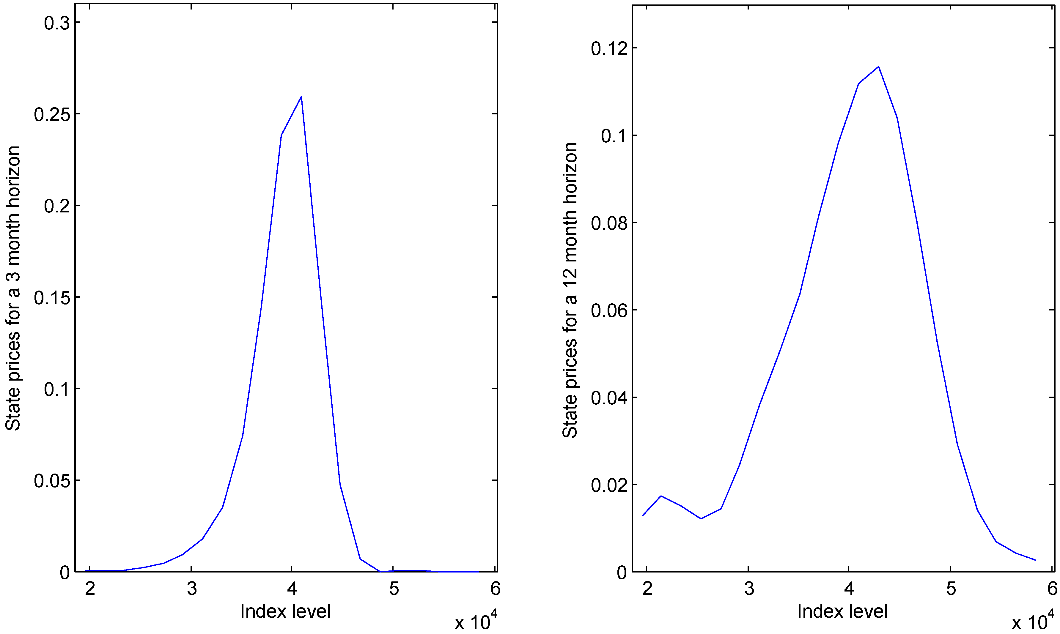
The specifics of the application are as follows. We work with a snapshot of data on 18 September 2013, when the FTSE/JSE Top40 was at 38,981.4. (Note that this is slightly different from the published value as the options were valued before the close of the day.) This becomes the eleventh entry $S_{11}$ of a $21\times 1$ column vector S, the entries of which we think of as the states. The intervals between the states are $5\%$ of $S_{11}$, so that $S_1=\frac{S_{11}}{2}$ and $S_{21}=\frac{3S_{11}}{2}$. We set $T=0.25$—this horizon of interest allows a few liquid derivatives to be relevant: for 3, 6, 9, 12 and 15 month expiries, we have nine call option premiums $H_i$ with the corresponding strikes $K_i$.

The smoothness-maximising method works well on this data—we obtain $p^{\left(0\right)}$, $p^{\left(T\right)}$, $p^{\left(2T\right)}$, $p^{\left(3T\right)}$, $p^{\left(4T\right)}$ and $p^{\left(5T\right)}$, two of which are shown in Figure 1. The bimodality seen in the longer-dated distribution is a typical feature, but in the absence of a recovery-type result, we cannot fully understand it: the market might assign significant probability to a crash, or it could be especially averse to this small risk.

In a similar vein, we begin the second sub-problem by writing restrictions on P. Consequently, $p^{\left(T\right)}$ becomes the middle row of P, i.e.,

$$\begin{array}{cc}& {\left(p^{\left(T\right)}\right)}^{\text{tr}}={\left(p^{\left(0\right)}\right)}^{\text{tr}}P.\hfill \end{array}$$

(10)

As we can only see the bond price relating to the current state, we cannot write a direct analogue to Equation (7). We enforce interest rate positivity though, and bond prices become endogenous to the problem. We can write an analogue to Equation (8), if we import the implied dividend yield from the current state. (Being a yield rather than an absolute amount, this seems a reasonable simplification.) These amount to, for each row $i=1,2,...,21$, enforcing

$$\begin{array}{cc}& \sum _{j=1}^{21}{p}_{ij}\le 1,\hfill \end{array}$$

(11)

$$\begin{array}{cc}& \sum _{j=1}^{21}{p}_{ij}{S}_j=S_i{e}^{-q^{\left(T\right)}T}.\hfill \end{array}$$

(12)

Setting $p_{i,0}=p_{i,22}=0$ for all i, define a smoothness function and a distance function by

$$\begin{array}{cc}& \mathcal{S}\left(P\right):=\sum _{i=1}^{21}\sum _{j=1}^{21}{(p_{i,j-1}-2p_{i,j}+p_{i,j+1})}^2,\hfill \\ & \mathcal{D}\left(P\right):=\sum _{k=1}^4(p^{\left(\right(k+1\left)T\right)}-p^{\left(kT\right)}P){(p^{\left(\right(k+1\left)T\right)}-p^{\left(kT\right)}P)}^{\text{tr}}.\hfill \end{array}$$

The state-price matrix is then determined with

$$\begin{array}{c}\hfill P=\underset{P\ge 0}{arg\; min}\left(\mathcal{S}\left(P\right)+\mathcal{D}\left(P\right)\right)\text{such}\text{that}\text{(}10\text{),}\text{(}11\text{)}\text{and}\text{(}12\text{)}\text{hold}.\end{array}$$

Note that we have minimised the squared errors in the few time-homogeneity equations, rather than enforce them strictly. There are many other ways that similar ideas could be applied, for example, by combining $\mathcal{S}$ and $\mathcal{P}$ differently.

Figure 1. Option-implied state prices for two horizons.

Figure 1. Option-implied state prices for two horizons.

The method turns out to work well (see two generic rows in Figure 2). Examining the left hand panel reveals a fragility though: because we set $p_{i,0}=p_{i,22}=0$, the smoothness metric pins the function down at zero on either side. As the bond price is not bounded below, pushing the peak towards the centre increases smoothness while maintaining Equation (12), causing high interest rates in the lower states. Adjusting the method to mitigate this causes other problems such as instability in the numerical optimisation, and it turns out to have a very small impact on the recovered distribution. In fact, rows farther from the middle are harder to determine, but are also less influential on the final result.

Figure 2. Two rows of the estimated state-price matrix.

Figure 2. Two rows of the estimated state-price matrix.

Here P satisfies the internal no-arbitrage condition, identified in ([6] p. 45), that the net carrying cost (interest minus dividends) must be positive in the lowest state, and negative in the highest (lest there be no downside in holding the index in the lowest state, or there be no upside in holding the index in the highest state).

As the Perron–Frobenius Theorem guarantees, F can be uniquely determined from P. Only the middle row is of direct interest and is shown in Figure 3. While our ability to derive this distribution is remarkable, it is quite difficult to test it or make concrete statements about its veracity. The realisation of the Top40 in 3 months’ time is the only relevant datum. One could look to come up with a hypothesis testing framework by repeating this exercise over many cross-sections in time, but it would be very difficult to avoid a test of low statistical power. We can take confidence in noting that the recovered distribution compares to the moment-matched log-normal density as we would expect: there is a heavier left tail and a sharper peak.

Figure 3. Recovered distribution and parametric comparison.

Figure 3. Recovered distribution and parametric comparison.

4. Conclusions

One may well ask about the extent to which Ross [1] should change our world view. The content of Remark 4 best summarises the revelatory nature of the Recovery Theorem—in this important sense, it does indeed change the world view of the author. However, whether the theorem is useful to the practitioner is a more difficult question. The assumptions, particularly the preference metastructure, are surely vast simplifications of reality, but, a priori at least, we cannot say whether this vitiates the result.

The curious reader might benefit from a few more references in addition to the papers mentioned so far. Of particular interest is the only thorough empirical study published at the time of writing: Audrino et al. [14], with a much bigger dataset than used here, assess the viability of simple market-timing strategies based on moments of a recovered distribution. Their implementation of the Recovery Theorem is not very different to that in Section 3. They employ a neural network technique, developed in [15], to translate available traded prices to appropriate sets of state prices—while this is not truly nonparametric like the smoothness method above, it is similar at a high level. Unlike Section 3, they rely solely on the time-homogeneity equations (embellished with a regularisation penalty) to populate the state-price matrix. Section 3 concentrated on implementation methodology, and therefore applied the Recovery Theorem at one particular, arbitrarily-chosen, point in time. We can gain insight from the recovery of distributions over a stretch of time in [14], firstly by noting that recovery appears to work in a fairly stable and regular manner. After some robustness checks, it is found that their strategies outperform the index on a risk-adjusted basis. With regard to the practical value of the Recovery Theorem, this analysis over a series of dates is encouraging.

While [6] derives a very simple continuous recovery result, Walden [16] and Qin and Linetsky [17] have done so with more sophistication. Walden [16] considers the recovery of real-world parameters from option prices where the stochastic driver is a one-dimensional time-homogeneous diffusion (with mild technical restrictions). The assumption of a transition-independent pricing kernel is made, but is stronger than in the context of this paper because the particular transition-independent form must hold for all future times t. By deriving a fundamental differential equation, a particular condition—which can be interpreted as the diffusion not being allowed to drift to positive or negative infinity too quickly—is found to be necessary and sufficient for recovery. Mean-reversion of the diffusion, or the existence of a stationary distribution, is sufficient but not necessary. Implementation of the method will be numerically intensive, in both calibrating the model to option prices and eliciting the solution. Qin and Linetsky [17] generalise this result by considering continuous-time Markov processes with general state spaces. Transition independence is similarly assumed, and the technical condition of recurrence of the driving process is found to be sufficient for recovery. A reader seeking full mathematical rigour might find this paper the appropriate next step.

In an interesting paper, Martin and Ross [18] examine long-dated bonds through the lens of the Recovery Theorem. This work is partially motivated by the difficulty of estimating P, and the authors find they can make some theoretical statements about long bonds independently of P. This work is related to the paper by Borovička et al. [19], which interrogates the Recovery Theorem from an econometric point of view and might interest readers looking for a deeper theoretical analysis.

In conclusion, this paper has, on the theoretical front, formalised, proved and discussed the Recovery Theorem, and added the extension of relaxation of state-independent preferences. The obstacles to application were then identified, which include definition of the state space and estimation of the state-price matrix. In the face of these, an implementation methodology was developed and executed. While the recovered distribution is subject to the model assumptions and application method, we conclude by noting that our ability to recover a distribution in this way is remarkable and represents an advancement in mathematical finance.