On a Discrete Interaction Risk Model with Delayed Claims

Abstract

We study a discrete-time interaction risk model with delayed claims within the framework of the compound binomial model. Using the technique of generating functions, we derive both a recursive formula and a defective renewal equation for the expected discounted penalty function. As applications, the probabilities of ruin and the joint distributions of the surplus one period to ruin and the deficit at ruin are investigated. Numerical illustrations are also given.

1. Introduction

In the last decade, risk models with time-correlated claims have been extensively studied in insurance and actuarial literature. For instance, see [1,2,3,4,5,6] and the reference therein. Among them, risk models with delayed claims (incurred, but not reported or reported, but not settled claims) have received considerable attention. Yuen and Guo [1] study a delayed claims risk model within the framework of the compound binomial model and obtain recursive formulas for the finite time ruin probabilities. Xiao and Guo [7] further investigate the aforementioned risk model and derive a recursive equation for the joint distribution of the surplus immediately prior to ruin and deficit at ruin. Bao and Liu [8] generalize the model in [1] by considering random premium income; both the probability of ultimate ruin and the joint distribution of the surplus prior to and at ruin are studied. When dividend payments are ruled by a constant dividend barrier in the model studied by [1], Wu and Li [9] investigate the expected present value of total dividends. Meanwhile, attention has also been paid to risk models whose aggregate claim process is a book of insurance business. For instance, see [10,11,12,13,14,15], among many others. In the case of two classes of business, Wu and Yuen [16] consider an interaction risk model with delayed claims and derive a recursive equation for the finite time survival probabilities. More results about risk models with delayed claim settlements can be found in [17,18,19].

In this paper, we propose a discrete-time interaction risk model that involves two classes of insurance claims, namely Class 1 and Class 2. In each time period, the probability of having a main claim in Class $i(i=1,2)$ is $p_i(0<p_i<1)$ and the probability of no main claim is $q_i=1-p_i$. Thus, the number of main claims in Class $i(i=1,2)$ is a binomial process $\{N_i\left(t\right),t\in \mathbb{N}\}$ with parameter $p_i$. Independence is assumed between $\{N_1\left(t\right),t\in \mathbb{N}\}$ and $\{N_2\left(t\right),t\in \mathbb{N}\}$. The claim amount random variables (r.v.s) in Class 1 and Class 2 are denoted by $\{X_j,j\in {\mathbb{N}}^{+}\}$ and $\{Y_j,j\in {\mathbb{N}}^{+}\}$, which are two sequences of independent and identically distributed (i.i.d.) positive and integer valued r.v.s. For $i,j\in \mathbb{N}$, we define

$$f_{ij}\left(k\right)=\mathrm{Pr}\left(\sum _{m=1}^i{X}_m+\sum _{n=1}^j{Y}_n=k\right),k\in \mathbb{N}.$$

(1)

The genetic r.v.s of $\{X_j,j\in {\mathbb{N}}^{+}\}$ and $\{Y_j,j\in {\mathbb{N}}^{+}\}$ are denoted by X and Y with mean ${\mu }_X$ and ${\mu }_Y$, respectively. It is assumed that each main claim in one class induces a by-claim in the other class. Each main claim in Class $i(i=1,2)$ and its associated by-claim in the other class may occur simultaneously with probability ${\rho }_i(0\le {\rho }_i\le 1)$ or the occurrence of the by-claim may be delayed to the next time period with probability ${\varrho }_i=1-{\rho }_i$.

Under the above assumptions, claims in each of the classes can be classified into two groups, one for main claims in the current class and one for by-claims induced by the main claims occurring in the other class. Note that the interaction comes from the assumption that main claims and by-claims within the same class are identically distributed. Although this assumption seems to be barely satisfactory, we imagine it could make sense in some special circumstances. For example, an insurer provides warehousing companies with a type of “full coverage” insurance. More precisely, risk management services are provided for: (i) the goods stored; and (ii) the warehouses of the company. In this case, a spontaneous fire of the goods might lead to an explosion and destroy the warehouses. On the other hand, a destruction of the warehouses would probably cause severe damage to the goods.

The total claim amount process is given by

$$S\left(t\right)=S_1\left(t\right)+S_2\left(t\right),t\in {\mathbb{N}}^{+},$$

where $S_i\left(t\right)(i=1,2)$ is the total claims (including main claims and by-claims) in Class i in the first t time period. If we suppose that the insurance company collects a unit amount of premium in each time period, then the surplus process can be written as

$$U_1\left(t\right)=u+t-S\left(t\right),t\in \mathbb{N},$$

(2)

where $U_1\left(0\right)=u$ is the initial surplus. This leads to the definition of the time of ruin

$$T=\left\{\begin{array}{ll}\min \left\{t>0,U_1\left(t\right)<0\right\},\hfill & \mathrm{if}\mathrm{such}\mathrm{a}t\mathrm{exists},\hfill \\ \infty ,\hfill & \mathrm{otherwise}.\hfill \end{array}\right.$$

It is obvious that $U_1(T-1)$ is the surplus one period prior to ruin, and $|U_1\left(T\right)|$ is the deficit at ruin. The expected discounted penalty function is defined as

$$m_1\left(u\right)=\mathrm{E}\left[v^{T}w\left(U_1(T-1),\left|U_1\left(T\right)\right|\right){\mathbf{1}}_{\{T<\infty \}}|U_1\left(0\right)=u\right].$$

Here, $v\in (0,1]$ is the one-period discount factor, $w:\mathbb{N}\times {\mathbb{N}}^{+}\to {\mathbb{R}}^{+}$ is the so-called penalty function and ${\mathbf{1}}_{\{·\}}$ is the indicator function.

It is not difficult to verify that $\mathrm{E}S\left(1\right)=\left(p_1+p_2{\rho }_2\right){\mu }_X+\left(p_1{\rho }_1+p_2\right){\mu }_Y$. Additionally, for $t=2,3,\dots$, it holds that

$$\begin{array}{cc}\hfill \mathrm{E}S\left(t\right)& =\mathrm{E}S(t-1)+(p_1+p_2)\left({\mu }_X+{\mu }_Y\right)\hfill \\ & =\left(p_1+p_2{\rho }_2\right){\mu }_X+\left(p_1{\rho }_1+p_2\right){\mu }_Y+\left(t-1\right)\left(p_1+p_2\right)\left({\mu }_X+{\mu }_Y\right).\hfill \end{array}$$

To guarantee that Equation (2) has a positive drift, we further assume

$$\left(p_1+p_2\right)\left({\mu }_X+{\mu }_Y\right)=1-\lambda ,$$

(3)

where $\lambda >0$ is the relative safety loading parameter.

The rest of paper is structured as follows. In Section 2, the explicit expression for the generating function of $m_1\left(u\right)$ is derived by introducing three supplementary surplus processes. In Section 3, we derive not only the recursive formula, but also the defective renewal equation for $m_1\left(u\right)$. Based on these results, the joint distributions of the surplus one period prior to ruin and the deficit at ruin, as well as the probabilities of ruin are studied in Section 4. Numerical illustrations are also given in Section 4.

2. The Generating Function of the Expected Discounted Penalty Function

To deal with $m_1\left(u\right)$ in detail, we need to define the following supplementary surplus processes

$$\begin{array}{cc}& U_2\left(t\right)=u+t-S\left(t\right)-\tilde{X},\hfill \end{array}$$

(4)

$$\begin{array}{cc}& U_3\left(t\right)=u+t-S\left(t\right)-\tilde{Y},\hfill \end{array}$$

(5)

$$\begin{array}{cc}& U_4\left(t\right)=u+t-S\left(t\right)-\tilde{X}-\tilde{Y},\hfill \end{array}$$

(6)

where $\tilde{X}$ and $\tilde{Y}$ are independent r.v.s having the same distribution function with X and Y, respectively. The expected discounted penalty function associated with the surplus process $\{U_i\left(t\right),t\in \mathbb{N}\}$ is denote by $m_i\left(u\right)$ for $1\le i\le 4$.

By conditioning on the occurrence (or not) of claims and their amounts (if necessary) in the next period in risk process Equation (2), one finds, for $u\in {\mathbb{N}}^{+}$,

$$\begin{array}{cc}\hfill m_1(u-1)& =v{q}_1{q}_2{m}_1\left(u\right)+v{p}_1{q}_2\left\{{\varrho }_1(m_3*f_{10}\left(u\right)+w_{10}\left(u\right))+{\rho }_1(m_1*f_{11}\left(u\right)+w_{11}\left(u\right))\right\}\hfill \\ & +v{q}_1{p}_2\left\{{\varrho }_2(m_2*f_{01}\left(u\right)+w_{01}\left(u\right))+{\rho }_2(m_1*f_{11}\left(u\right)+w_{11}\left(u\right))\right\}\hfill \\ & +v{p}_1{p}_2\{{\varrho }_1{\varrho }_2(m_4*f_{11}\left(u\right)+w_{11}\left(u\right))+{\varrho }_1{\rho }_2(m_3*f_{21}\left(u\right)+w_{21}\left(u\right))\hfill \\ & +{\rho }_1{\varrho }_2(m_2*f_{12}\left(u\right)+w_{12}\left(u\right))+{\rho }_1{\rho }_2(m_1*f_{22}\left(u\right)+w_{22}\left(u\right))\},\hfill \end{array}$$

(7)

where * is the convolution factor, $f_{ij}$ is the probability mass function defined by Equation (1) and

$$w_{ij}\left(u\right)=\left\{\begin{array}{cc}0,\hfill & u=0,\hfill \\ \sum _{k=u+1}^{\infty }w(u-1,k-u)f_{ij}\left(k\right),\hfill & u=1,2,\dots ,\hfill \end{array}\right.$$

For $k\in \mathbb{N}$, we define

$$\begin{array}{cc}\hfill {\gamma }_1\left(k\right)& =\left(p_1{q}_2{\rho }_1+q_1{p}_2{\rho }_2\right)f_{11}(k+1)+p_1{p}_2{\rho }_1{\rho }_2{f}_{22}(k+1),\hfill \\ \hfill {\gamma }_2\left(k\right)& =p_2{\varrho }_2\left(q_1{f}_{01}(k+1)+p_1{\rho }_1{f}_{12}(k+1)\right),\hfill \\ \hfill {\gamma }_3\left(k\right)& =p_1{\varrho }_1\left(q_2{f}_{10}(k+1)+p_2{\rho }_2{f}_{21}(k+1)\right),\hfill \\ \hfill {\gamma }_4\left(k\right)& =p_1{p}_2{\varrho }_1{\varrho }_2{f}_{11}(k+1),\hfill \end{array}$$

then Equation (7) can be rewritten as

$$\begin{array}{cc}\hfill \frac{1}{v}{m}_1(u-1)=& q_1{q}_2{m}_1\left(u\right)+\sum _{i=1}^4{m}_i*{\gamma }_i(u-1)+{\mathit{\sigma }}_1\left(u\right)\mathit{p},\hfill \end{array}$$

(8)

where

$$\begin{array}{c}{\mathit{\sigma }}_1\left(u\right)=\left(0,w_{10}\left(u\right),w_{01}\left(u\right),w_{11}\left(u\right),w_{21}\left(u\right),w_{12}\left(u\right),w_{22}\left(u\right)\right),\\ \mathit{p}={\left(q_1{q}_2,p_1{q}_2{\varrho }_1,q_1{p}_2{\varrho }_2,p_1{q}_2{\rho }_1+q_1{p}_2{\rho }_2+p_1{p}_2{\varrho }_1{\varrho }_2,p_1{p}_2{\varrho }_1{\rho }_2,p_1{p}_2{\rho }_1{\varrho }_2,p_1{p}_2{\rho }_1{\rho }_2\right)}^{\text{T}}.\end{array}$$

We use the technique of generating functions to investigate the expected discounted penalty function. The generating function of a function f is denoted by adding a hat on the corresponding letter, i.e., $\widehat{f}\left(z\right)={\sum }_{k=0}^{\infty }{z}^{k}f\left(k\right)$. Moreover, if $\mathit{A}\left(k\right)={\left(a_{ij}\left(k\right)\right)}_{m\times n}$ is a $m\times n$ matrix with $a_{ij}\left(k\right)$ $(1\le i\le m,1\le j\le n)$ being its elements, then $\widehat{\mathit{A}}\left(z\right)={\sum }_{k=0}^{\infty }{z}^k\mathit{A}\left(k\right)={\left({\widehat{a}}_{ij}\left(z\right)\right)}_{m\times n}$.

Multiplying both sides of Equation (8) by $z^u$ and summing over u from 1 to ∞ yields

$$\frac{z}{v}{\widehat{m}}_1\left(z\right)=q_1{q}_2\left({\widehat{m}}_1\left(z\right)-m_1\left(0\right)\right)+z{\widehat{\gamma }}_{14}\left(z\right){\widehat{\mathit{m}}}_{14}\left(z\right)+{\widehat{\mathit{\sigma }}}_1\left(z\right)\mathit{p},$$

(9)

where ${\mathit{m}}_{ij}\left(k\right)={\left(m_i\left(k\right),\dots ,m_j\left(k\right)\right)}^{\text{T}}$ and ${\gamma }_{ij}\left(k\right)=\left({\gamma }_i\left(k\right),\dots ,{\gamma }_j\left(k\right)\right)$ for $1\le i\le j\le 4$.

Similar to the derivation of Equation (9), it can be obtained from the supplementary surplus processes Equations (4)–(6) that

$$\frac{z}{v}{\widehat{\mathit{m}}}_{24}\left(z\right)=\left(q_1{q}_2{\widehat{m}}_1\left(z\right)+z{\widehat{\gamma }}_{14}\left(z\right){\widehat{\mathit{m}}}_{14}\left(z\right)\right)\left(\begin{array}{c}{\widehat{f}}_{10}\left(z\right)\\ {\widehat{f}}_{01}\left(z\right)\\ {\widehat{f}}_{11}\left(z\right)\end{array}\right)+\left(\begin{array}{c}{\widehat{\mathit{\sigma }}}_2\left(z\right)\\ {\widehat{\mathit{\sigma }}}_3\left(z\right)\\ {\widehat{\mathit{\sigma }}}_4\left(z\right)\end{array}\right)\mathit{p},$$

(10)

where

$$\begin{array}{c}\hfill {\mathit{\sigma }}_2\left(k\right)=\left(w_{10}\left(k\right),w_{20}\left(z\right),w_{11}\left(k\right),w_{21}\left(k\right),w_{31}\left(k\right),w_{22}\left(k\right),w_{32}\left(k\right)\right),\\ \hfill {\mathit{\sigma }}_3\left(k\right)=\left(w_{01}\left(k\right),w_{11}\left(z\right),w_{02}\left(k\right),w_{12}\left(k\right),w_{22}\left(k\right),w_{13}\left(k\right),w_{23}\left(k\right)\right),\\ \hfill {\mathit{\sigma }}_4\left(k\right)=\left(w_{11}\left(k\right),w_{21}\left(z\right),w_{12}\left(k\right),w_{22}\left(k\right),w_{32}\left(k\right),w_{23}\left(k\right),w_{33}\left(k\right)\right).\end{array}$$

On the other hand, it is known from Equation (9) that

$$q_1{q}_2{\widehat{m}}_1\left(z\right)+z{\widehat{\gamma }}_{14}\left(z\right){\widehat{\mathit{m}}}_{14}\left(z\right)=\frac{z}{v}{\widehat{m}}_1\left(z\right)+q_1{q}_2{m}_1\left(0\right)-{\widehat{\mathit{\sigma }}}_1\left(z\right)\mathit{p}.$$

(11)

Substituting Equation (11) into Equation (10) yields

$$\frac{z}{v}{\widehat{\mathit{m}}}_{24}\left(z\right)=\left(\frac{z}{v}{\widehat{m}}_1\left(z\right)+q_1{q}_2{m}_1\left(0\right)-{\widehat{\mathit{\sigma }}}_1\left(z\right)\mathit{p}\right)\widehat{\mathit{f}}\left(z\right)+{\widehat{\mathit{\sigma }}}_{24}\left(z\right)\mathit{p},$$

(12)

where $\mathit{f}\left(k\right)={\left(f_{10}\left(k\right),f_{01}\left(k\right),f_{11}\left(k\right)\right)}^{\text{T}}$ and ${\mathit{\sigma }}_{ij}\left(k\right)={\left({\mathit{\sigma }}_i\left(k\right),\dots ,{\mathit{\sigma }}_j\left(k\right)\right)}^{\text{T}}$ for $1\le i\le j\le 4$.

To give the explicit expression for the generating function of the expected discounted penalty function, we define

$$\begin{array}{c}g\left(k\right)=(p_1{q}_2+q_1{p}_2)f_{11}(k+1)+p_1{p}_2{f}_{22}(k+1),\\ h\left(k\right)=(p_1{q}_2{\varrho }_1+q_1{p}_2{\varrho }_2)f_{11}(k+1)+p_1{p}_2(1-{\rho }_1{\rho }_2)f_{22}(k+1),\end{array}$$

with $G\left(k\right)={\sum }_{i=0}^{k}g\left(j\right)$ and $H\left(k\right)={\sum }_{i=0}^{k}h\left(k\right)$ being the (defective) distribution functions of g and h, respectively. Then, it is easy to see that

$$\widehat{g}\left(z\right)={\widehat{\gamma }}_1\left(z\right)+{\widehat{\gamma }}_{24}\left(z\right)\widehat{\mathit{f}}\left(z\right)\mathrm{and}\widehat{h}\left(z\right)={\widehat{\gamma }}_{24}\left(z\right)\widehat{\mathit{f}}\left(z\right).$$

For the rest of the paper, we denote by $m\left(u\right)=m_1\left(u\right)$ for $u\in \mathbb{N}$. Then, combining Equations (9) and (12) yields

$$\begin{array}{c}\hfill \widehat{m}\left(z\right)=\frac{v{\widehat{\mathit{\gamma }}}_{24}\left(z\right){\widehat{\sigma }}_{24}\left(z\right)\mathit{p}-(1-v\widehat{h}\left(z\right))(q_1{q}_{2}m\left(0\right)-{\widehat{\mathit{\sigma }}}_1\left(z\right)\mathit{p})}{\frac{z}{v}-q_1{q}_2-z\widehat{g}\left(z\right)}.\end{array}$$

(13)

In order to determine the constant $m\left(0\right)$, we need to investigate the so-called Lundberg’s fundamental equation defined as

$$z\widehat{g}\left(z\right)=\frac{z}{v}-q_1{q}_2.$$

(14)

Lemma 1. The Lundberg’s fundamental Equation (14) has exactly two roots, say $z=r\in (v{q}_1{q}_2,v]$ and $z=R\in (1,\infty )$.

Proof. It is easy to verify that ${\left(z\widehat{g}\left(z\right)\right)}^{\prime }>0$ and ${\left(z\widehat{g}\left(z\right)\right)}^{\prime \prime }>0$, which implies that $z\widehat{g}\left(z\right)$ is an increasing convex function. Hence, Equation (14) has at most two roots. By noting that

$$\begin{array}{c}v{q}_1{q}_2\widehat{g}\left(v{q}_1{q}_2\right)>0={\left(\frac{z}{v}-q_1{q}_2\right)}_{z=v{q}_1{q}_2},\\ v\widehat{g}\left(v\right)\le \widehat{g}\left(1\right)=p_1{q}_2+q_1{p}_2+p_1{p}_2={\left(\frac{z}{v}-q_1{q}_2\right)}_{z=v},\end{array}$$

we conclude that there is a root $z=r\in (v{q}_1{q}_2,v]$ to Equation (14). Moreover, it is known from the safety loading condition Equation (3) that

$${\left(z\widehat{g}\left(z\right)\right)}_{z=1}^{\prime }=\left(p_1+p_2\right)\left({\mu }_X+{\mu }_Y\right)<1\le \frac{1}{v}={\left(\frac{z}{v}-q_1{q}_2\right)}^{\prime },$$

which yields that there exists another real number $z=R\in (1,\infty )$, such that $z\widehat{g}\left(z\right)=\frac{z}{v}-q_1{q}_2$.  ☐

Setting $z=r$ in Equation (13), we can derive an expression for $m\left(0\right)$.

Theorem 1. When the initial surplus is zero, the expected discounted penalty function can be calculated by

$$m\left(0\right)=\frac{1}{q_1{q}_2}\left({\widehat{\mathit{\sigma }}}_1\left(r\right)+\frac{v}{1-v\widehat{h}\left(r\right)}{\widehat{\gamma }}_{24}\left(r\right){\widehat{\mathit{\sigma }}}_{24}\left(r\right)\right)\mathit{p}.$$

(15)

To end this section, we conclude that an explicit expression for the generating function of $m\left(u\right)$ is given by Equation (13), where the constant $m\left(0\right)$ is determined by Equation (15).

3. Recursive Equations for $\mathit{m}\left(\mathit{u}\right)$

In this part, we show that $m\left(u\right)$ can be calculated by a recursive equation, from which the defective renewal equation for $m\left(u\right)$ can be obtained.

Theorem 2. For $u\in {\mathbb{N}}^{+}$, it holds that

$$\begin{array}{c}\hfill q_1{q}_{2}m\left(u\right)=\frac{1}{v}m(u-1)-m*g(u-1)-v{q}_1{q}_{2}m\left(0\right)h\left(u\right)-{\zeta }_v\left(u\right)\mathit{p},\end{array}$$

(16)

where

$${\zeta }_v\left(u\right)={\mathit{\sigma }}_1\left(u\right)-v\sum _{n=0}^u\left(h(u-n){\mathit{\sigma }}_1\left(n\right)-{\gamma }_{24}(u-n){\mathit{\sigma }}_{24}\left(n\right)\right),$$

and the constant $m\left(0\right)$ can be determined by Equation (15).

Proof. It is known from Equation (13) that

$$\begin{array}{cc}\hfill \left(\frac{z}{v}-z\widehat{g}\left(z\right)\right)\widehat{m}\left(z\right)=& q_1{q}_2\left(\widehat{m}\left(z\right)-m\left(0\right)\right)+v{q}_1{q}_{2}m\left(0\right)\widehat{h}\left(z\right)\hfill \\ & +\left(1-v\widehat{h}\left(z\right)\right){\widehat{\mathit{\sigma }}}_1\left(z\right)\mathit{p}+v{\widehat{\gamma }}_{24}\left(z\right){\widehat{\mathit{\sigma }}}_{24}\left(z\right)\mathit{p}.\hfill \end{array}$$

(17)

After some modification, one could see that Equation (17) is equivalent to

$$\begin{array}{cc}& \sum _{u=1}^{\infty }{z}^u\left\{\frac{1}{v}m(u-1)-m*g(u-1)\right\}-q_1{q}_2\sum _{u=1}^{\infty }{z}^u\left(m\left(u\right)+vm\left(0\right)h\left(u\right)\right)\hfill \\ & =\sum _{u=1}^{\infty }{z}^u\left\{{\mathit{\sigma }}_1\left(u\right)-v\sum _{n=0}^u\left(h(u-n){\mathit{\sigma }}_1\left(n\right)-{\gamma }_{24}(u-n){\mathit{\sigma }}_{24}\left(n\right)\right)\right\}\mathit{p},\hfill \end{array}$$

which yields Equation (16) by comparing the coefficients of $z^u$. ☐

Now, we are in a position to derive the defective renewal equation for $m\left(u\right)$. It is known from Equation (16) that

$$\begin{array}{cc}\hfill q_1{q}_2\left(m\left(k\right)-\frac{1}{r}m(k-1)\right)=& \left(\frac{1}{v}-q_1{q}_2\frac{1}{r}\right)m(k-1)-\sum _{i+j=k-1}m\left(i\right)g\left(j\right)\hfill \\ & -v{q}_1{q}_{2}m\left(0\right)h\left(k\right)-{\zeta }_v\left(k\right)\mathit{p}.\hfill \end{array}$$

(18)

Multiplying both sides of Equation (18) by $r^k$ and summing over k from one to u yields

$$\begin{array}{cc}\hfill q_1{q}_2(r^{u}m\left(u\right)-m\left(0\right))=& \left(\frac{r}{v}-q_1{q}_2\right)\sum _{k=0}^{u-1}{r}^{k}m\left(k\right)-r\sum _{k=0}^{u-1}{r}^{k}m\left(k\right)\sum _{j=0}^{u-1-k}{r}^{j}g\left(j\right)\hfill \\ & -v{q}_1{q}_{2}m\left(0\right)\sum _{k=1}^u{r}^{k}h\left(k\right)-\sum _{k=1}^u{r}^k{\zeta }_v\left(k\right)\mathit{p},\hfill \end{array}$$

which can be rewritten as

$$\begin{array}{cc}\hfill \frac{1}{v}{r}^{u+1}m\left(u\right)=& \sum _{k=0}^u{r}^{k}m\left(k\right)\left\{\frac{r}{v}-q_1{q}_2-r\sum _{j=0}^{u-1-k}{r}^{j}g\left(j\right)\right\}\hfill \\ & +q_1{q}_{2}m\left(0\right)\left(1-v\sum _{k=0}^u{r}^{k}h\left(k\right)\right)-\sum _{k=1}^u{r}^k{\zeta }_v\left(k\right)\mathit{p}.\hfill \end{array}$$

(19)

Substituting Equation (14) into Equation (19), we get

$$\begin{array}{cc}\hfill m\left(u\right)=& v\sum _{k=0}^{u}m(u-k)\sum _{j=0}^{\infty }{r}^{j}g(j+k)\hfill \\ & +v{r}^{-(u+1)}\left\{q_1{q}_{2}m\left(0\right)\left(1-v\sum _{k=0}^u{r}^{k}h\left(k\right)\right)-\sum _{k=1}^u{r}^k{\zeta }_v\left(k\right)\mathit{p}\right\}.\hfill \end{array}$$

(20)

To simplify the right-hand side of Equation (20), we define the following auxiliary functions:

$$\begin{array}{c}{\mathit{\alpha }}_v(u,k)={\mathit{\sigma }}_1\left(k\right)-v\sum _{j=0}^{u}h\left(j\right){\mathit{\sigma }}_1(k-j),\end{array}$$

(21)

$$\begin{array}{c}{\beta }_v(u,k)=\sum _{m+n=k}{\mathit{\gamma }}_{24}\left(m\right){\sigma }_{24}\left(n\right)-v\left({\mathit{\delta }}_1(u,k)-{\mathit{\delta }}_2(u,k)\right),\end{array}$$

(22)

where

$$\begin{array}{cc}\hfill {\mathit{\delta }}_1(u,k)& =\sum _{j=0}^{u}h\left(j\right)\sum _{m+n=k-j}{\gamma }_{24}\left(m\right){\mathit{\sigma }}_{24}\left(n\right),\hfill \\ \hfill {\mathit{\delta }}_2(u,k)& =\sum _{j=0}^{u}h(k-j)\sum _{m+n=j}{\gamma }_{24}\left(m\right){\mathit{\sigma }}_{24}\left(n\right).\hfill \end{array}$$

After some algebra, we know from Equation (15) that

$$q_1{q}_{2}m\left(0\right)\left(1-v\sum _{k=0}^u{r}^{k}h\left(k\right)\right)-\sum _{k=1}^u{r}^k{\zeta }_v\left(k\right)\mathit{p}=\sum _{k=u+1}^{\infty }{r}^k\left({\mathit{\alpha }}_v(u,k)+\frac{v{\beta }_v(u,k)}{1-v\widehat{h}\left(r\right)}\right)\mathit{p}.$$

(23)

Hence, substituting Equation (23) into Equation (20) yields the following result for $m\left(u\right)$.

Theorem 3. For $u\in \mathbb{N}$, it holds that

$$m\left(u\right)=v\sum _{k=0}^{u}m(u-k)\sum _{j=0}^{\infty }{r}^{j}g(j+k)+v\sum _{k=u+1}^{\infty }{r}^{k-u-1}\left({\alpha }_v(u,k)+\frac{v{\beta }_v(u,k)}{1-v\widehat{h}\left(r\right)}\right)\mathit{p}.$$

(24)

Now, we demonstrate that the renewal Equation (24) is defective. When $v<1$, we obtain by reversing the order of summation:

$$\begin{array}{cc}\hfill \sum _{k=0}^{\infty }\left(v\sum _{j=0}^{\infty }{r}^{j}g(j+k)\right)& =v\sum _{k=0}^{\infty }\sum _{j=k}^{\infty }{r}^{j-k}g\left(j\right)=\frac{v}{1-r}\left(\sum _{k=0}^{\infty }g\left(k\right)-r\widehat{g}\left(r\right)\right)\hfill \\ & =\frac{v}{1-r}\left(1-q_1{q}_2-\left(\frac{r}{v}-q_1{q}_2\right)\right)=\frac{v-r}{1-r}<1.\hfill \end{array}$$

(25)

When $v\to 1^{-}$, it is easy to see that

$$\underset{v\to 1^{-}}{lim}r=1.$$

(26)

Consequently, we know from the safety loading condition that

$$\sum _{k=0}^{\infty }\left(\underset{v\to 1^{-}}{lim}v\sum _{j=0}^{\infty }{r}^{j}g(j+k)\right)=\sum _{k=0}^{\infty }\sum _{j=k}^{\infty }g\left(j\right)=(p_1+p_2)\left({\mu }_X+{\mu }_Y\right)<1.$$

(27)

Therefore, we conclude from Equations (25) and (27) that Equation (24) is a defective renewal equation.

It is obvious that the values of $m\left(u\right)$ can be recursively evaluated by Equation (16) or Equation (24). Moreover, applying Equation (16) in a recursive procedure seems to be much easier than applying Equation (24). However, the defective renewal Equation (24) can be used to deduce both a compound geometric tail expression and an asymptotic estimate for $m\left(u\right)$ (see, for instance, [20], in which the analogue results are obtained for probabilities of ruin in the classical risk model).

4. Ruin-Related Quantities

In this section, we investigate some ruin-related quantities. For $u\in \mathbb{N}$, denote by

$$\begin{array}{cc}\hfill \psi \left(u\right)& =\mathrm{Pr}\left\{T<\infty |U_1\left(0\right)=u\right\},\hfill \end{array}$$

the probabilities of ruin. For $u\in \mathbb{N}$ and $(x,y)\in \mathbb{N}\times {\mathbb{N}}^{+}$, let

$$\begin{array}{cc}\hfill \phi (u,x,y)& =\mathrm{Pr}\left\{U_1(T-1)=x,|U_1\left(T\right)|=y,T<\infty |U_1\left(0\right)=u\right\},\hfill \end{array}$$

be the joint distribution of the surplus one period prior to ruin and the deficit at ruin. Then, it is obvious that $\psi \left(u\right)={\sum }_{(x,y)\in \mathbb{N}\times {\mathbb{N}}^{+}}\phi (u,x,y),u\in \mathbb{N}$.

4.1. The Evaluation of $\phi (u,x,y)$

Throughout this part, it is assumed that $v\to 1^{-}$ and $w(m,n)={\mathbf{1}}_{\{m=x,n=y\}}$, $(m,n)\in \mathbb{N}\times {\mathbb{N}}^{+}$. In this special case, we have $m\left(u\right)=\phi (u,x,y)$ for $u\in \mathbb{N}$. By noting

$$w_{ij}\left(u\right)=\left\{\begin{array}{cc}0,\hfill & u=0,\hfill \\ f_{ij}(x+y+1){\mathbf{1}}_{\{u=x+1\}},\hfill & u=1,2,\dots ,\hfill \end{array}\right.$$

(28)

we define the following auxiliary functions

$$\begin{array}{cc}\hfill D_1(x,y)& =(p_1{q}_2{\varrho }_1{f}_{10}+q_1{p}_2{\varrho }_2{f}_{01}+(p_1{q}_2{\rho }_1+q_1{p}_2{\rho }_2+p_1{p}_2{\varrho }_1{\varrho }_2)f_{11}\hfill \\ & +p_1{p}_2{\varrho }_1{\rho }_2{f}_{21}+p_1{p}_2{\rho }_1{\varrho }_2{f}_{12}+p_1{p}_2{\rho }_1{\rho }_2{f}_{22})\otimes (x+y+1),\hfill \\ \hfill D_2(x,y)& =(q_1{q}_2{f}_{10}+p_1{q}_2{\varrho }_1{f}_{20}+q_1{p}_2{\varrho }_2{f}_{11}+(p_1{q}_2{\rho }_1+q_1{p}_2{\rho }_2+p_1{p}_2{\varrho }_1{\varrho }_2)f_{21}\hfill \\ & +p_1{p}_2{\varrho }_1{\rho }_2{f}_{31}+p_1{p}_2{\rho }_1{\varrho }_2{f}_{22}+p_1{p}_2{\rho }_1{\rho }_2{f}_{32})\otimes (x+y+1),\hfill \\ \hfill D_3(x,y)& =(q_1{q}_2{f}_{01}+p_1{q}_2{\varrho }_1{f}_{11}+q_1{p}_2{\varrho }_2{f}_{02}+(p_1{q}_2{\rho }_1+q_1{p}_2{\rho }_2+p_1{p}_2{\varrho }_1{\varrho }_2)f_{12}\hfill \\ & +p_1{p}_2{\varrho }_1{\rho }_2{f}_{22}+p_1{p}_2{\rho }_1{\varrho }_2{f}_{13}+p_1{p}_2{\rho }_1{\rho }_2{f}_{23})\otimes (x+y+1),\hfill \\ \hfill D_4(x,y)& =(q_1{q}_2{f}_{11}+p_1{q}_2{\varrho }_1{f}_{21}+q_1{p}_2{\varrho }_2{f}_{12}+(p_1{q}_2{\rho }_1+q_1{p}_2{\rho }_2+p_1{p}_2{\varrho }_1{\varrho }_2)f_{22}\hfill \\ & +p_1{p}_2{\varrho }_1{\rho }_2{f}_{32}+p_1{p}_2{\rho }_1{\varrho }_2{f}_{23}+p_1{p}_2{\rho }_1{\rho }_2{f}_{33})\otimes (x+y+1),\hfill \end{array}$$

where $\left({\sum }_{j=1}^n{c}_j{f}_j\right)\otimes \left(k\right)={\sum }_{j=1}^n{c}_j{f}_j\left(k\right)$, $n\in {\mathbb{N}}^{+}$ for any coefficients $c_j(j=1,\dots ,n)$ and functions $f_j(j=1,\dots ,n)$. Then, it is known from Equation (28) that

$$\begin{array}{cc}& {\widehat{\mathit{\sigma }}}_i\left(1\right)\mathit{p}=D_i(x,y),\hfill \end{array}$$

(29)

$$\begin{array}{cc}& {\mathit{\sigma }}_i\left(k\right)\mathit{p}={\mathbf{1}}_{\{k=x+1\}}{D}_i(x,y),k\in {\mathbb{N}}^{+},\hfill \end{array}$$

(30)

and

$$\sum _{j=0}^k{\gamma }_i(k-j){\sigma }_i\left(j\right)\mathbf{p}={\mathbf{1}}_{\{k\ge x+1\}}{\gamma }_i(k-1-x)D_i(x,y),k\in {\mathbb{N}}^{+}.$$

(31)

for $1\le i\le 4$. Hence, substituting Equation (29) into Equation (15) yields

$$\phi (0,x,y)=\frac{1}{q_1{q}_2}\left({\mathit{D}}_1(x,y)+\frac{1}{\pi }\mathit{q}{\mathbf{D}}_{24}(x,y)\right),$$

(32)

where

$$\begin{array}{c}\pi =1-\widehat{h}\left(1\right)=(1-p_1{\varrho }_1)(1-p_2{\varrho }_2),\\ \mathit{q}={\widehat{\gamma }}_{24}\left(1\right)=\left(p_2{\varrho }_2(p_1{\rho }_1+q_1),p_1{\varrho }_1(p_2{\rho }_2+q_2),p_1{p}_2{\varrho }_1{\varrho }_2\right),\\ {\mathit{D}}_{ij}(x,y)={\left(D_i(x,y),\dots ,D_j(x,y)\right)}^{\text{T}},1\le i\le j\le 4.\end{array}$$

Similarly, we know from Equations (16), (26) and (30) that

$$\begin{array}{cc}\hfill q_1{q}_2\phi (u,x,y)=& \phi (u-1,x,y)-\sum _{k=0}^{u-1}\phi (k,x,y)g(u-1-k)-q_1{q}_2\phi (0,x,y)h\left(u\right)\hfill \\ & +\left(h(u-1-x)D_1(x,y)-{\gamma }_{24}(u-1-x){\mathit{D}}_{24}(x,y)\right){\mathbf{1}}_{\{u\ge x+1\}}\hfill \\ & -D_1(x,y){\mathbf{1}}_{\{u=x+1\}}.\hfill \end{array}$$

(33)

We remark that Equations (14) and (21) in [7] are recovered by Equations (32) and (33) in the present paper with $p_2=0$, respectively.

It is notable that the defective renewal equation for $\phi (u,x,y)$ can also be obtained. In the case of $w(m,n)={\mathbf{1}}_{\{m=x,n=y\}}$, we know from Equation (30) that

$$\begin{array}{cc}\hfill \sum _{k=u+1}^{\infty }{\mathit{\alpha }}_1(u,k)\mathit{p}& =\left({\mathbf{1}}_{\{u\le x\}}-\sum _{k=max\{0,u-x\}}^{u}h\left(k\right)\right)D_1(x,y)\hfill \\ & =\left({\mathbf{1}}_{\{u\le x\}}+H(u-1-x)-H\left(u\right)\right)D_1(x,y).\hfill \end{array}$$

(34)

Similarly, it is not difficult to verify that

$$\begin{array}{c}\sum _{k=u+1}^{\infty }\sum _{m+n=k}{\mathit{\gamma }}_{24}\left(m\right){\sigma }_{24}\left(n\right)\mathit{p}=\left(\mathit{q}-\sum _{k=0}^{u-x-1}{\gamma }_{24}\left(k\right)\right){\mathit{D}}_{24}(x,y),\\ \sum _{k=u+1}^{\infty }{\mathit{\delta }}_1(u,k)\mathit{p}=\left(H\left(u\right)\mathit{q}-\sum _{k=0}^{u-x-1}H(u-1-x-k){\gamma }_{24}\left(k\right)\right){\mathit{D}}_{24}(x,y),\\ \sum _{k=u+1}^{\infty }{\mathit{\delta }}_2(u,k)\mathit{p}=\sum _{k=0}^{u-1-x}\overline{H}(u-1-x-k){\gamma }_{24}\left(k\right){\mathit{D}}_{24}(x,y),\end{array}$$

and consequently,

$$\begin{array}{c}\hfill \sum _{k=u+1}^{\infty }{\beta }_1(u,k)\mathit{p}=\left\{\left(1-H\left(u\right)\right)\mathit{q}-\pi \sum _{k=0}^{u-1-x}{\gamma }_{24}\left(k\right)\right\}{\mathit{D}}_{24}(x,y).\end{array}$$

(35)

Substituting Equations (26), (34) and (35) into Equation (24) yields the defective renewal equation for $\phi (u,x,y)$ as follows:

$$\begin{array}{cc}\hfill \phi (u,x,y)=& \sum _{k=0}^u\phi (u-k,x,y)\overline{G}(k-1)+\left\{{\mathbf{1}}_{\{u\le x\}}+H(u-1-x)-H\left(u\right)\right\}{D}_1(x,y)\hfill \\ & +\left\{\frac{1-H\left(u\right)}{\pi }\mathit{q}-\sum _{k=0}^{u-1-x}{\gamma }_{24}\left(k\right)\right\}{\mathit{D}}_{24}(x,y),\hfill \end{array}$$

(36)

where $\overline{G}$ and $\overline{H}$ are tails of G and H, i.e., $\overline{G}\left(k\right)=1-q_1{q}_2-G\left(k\right),\overline{H}\left(k\right)=p_1{\varrho }_1+p_2{\varrho }_2-p_1{p}_2{\varrho }_1{\varrho }_2-H\left(k\right)$ for $k\in \mathbb{N}$.

Example 1. Suppose that claim amount r.v.s in both of the two classes are zero-truncated geometrically distributed with

$$\mathrm{Pr}\{X=k\}=(1-a)a^{k-1},\mathrm{Pr}\{Y=k\}=(1-b)b^{k-1},$$

for $k\in {\mathbb{N}}^{+}$ and $0<a,b<1$. If we set $p_1=0.1$, $p_2=0.2$, $a=1/3$ and $b=1/4$, then it easy to see that

$$\left(p_1+p_2\right)\left({\mu }_X+{\mu }_Y\right)=0.85<1,$$

which ensures that the safety loading condition Equation (3) holds. The numerical results of $\phi (u,x,y)$ are given in Table 1.

Table 1. The values of $\phi (u,x,y)$ with $p_1=0.1,p_2=0.2,a=1/3$ and $b=1/4$.

$(x,y)$	$({\rho }_1,{\rho }_2)$	$u=0$	$u=1$	$u=2$	$u=4$	$u=7$	$u=11$
(0, 1)	(0, 0)	0.2411265	0.1440916	0.1242079	0.0978323	0.0697250	0.0443761
	(0.2, 0.3)	0.2016123	0.1048111	0.0925975	0.0735956	0.0524333	0.0333685
	(0.7, 0.6)	0.1760715	0.0747127	0.0679853	0.0545247	0.0388603	0.0247297
	(1, 1)	0.1805556	0.0702160	0.0649220	0.0524670	0.0375076	0.0238703
(2, 2)	(0, 0)	0.0172947	0.0217721	0.0258049	0.0181552	0.0127906	0.0081399
	(0.2, 0.3)	0.0220675	0.0285528	0.0344494	0.0216139	0.0153322	0.0097567
	(0.7, 0.6)	0.0255570	0.0342691	0.0422659	0.0244623	0.0174832	0.0111258
	(1, 1)	0.0263873	0.0366490	0.0461370	0.0257016	0.0184810	0.0117674
(0, 5)	(0, 0)	0.0067270	0.0052610	0.0045711	0.0035766	0.0025444	0.0016194
	(0.2, 0.3)	0.0098012	0.0060842	0.0053607	0.0042411	0.0030194	0.0019216
	(0.7, 0.6)	0.0121226	0.0058755	0.0053210	0.0042648	0.0030384	0.0019335
	(1, 1)	0.0127322	0.0049514	0.0045781	0.0036998	0.0026449	0.0016832
(4, 2)	(0, 0)	0.0025660	0.0032303	0.0038286	0.0048460	0.0032192	0.0020417
	(0.2, 0.3)	0.0042676	0.0055218	0.0066621	0.0085932	0.0052395	0.0033295
	(0.7, 0.6)	0.0055996	0.0075085	0.0092606	0.0122356	0.0070499	0.0044883
	(1, 1)	0.0059314	0.0082381	0.0103709	0.0140154	0.0077988	0.0049779
(3, 5)	(0, 0)	0.0003576	0.0004502	0.0005336	0.0005255	0.0003656	0.0002324
	(0.2, 0.3)	0.0007714	0.0009981	0.0012042	0.0010776	0.0007582	0.0004823
	(0.7, 0.6)	0.0011091	0.0014871	0.0018341	0.0015225	0.0010926	0.0006952
	(1, 1)	0.0011517	0.0015995	0.0020136	0.0015696	0.0011413	0.0007273
(5, 3)	(0, 0)	0.0003576	0.0004502	0.0005336	0.0006754	0.0005648	0.0003558
	(0.2, 0.3)	0.0007714	0.0009981	0.0012042	0.0015533	0.0012039	0.0007628
	(0.7, 0.6)	0.0011091	0.0014871	0.0018341	0.0024234	0.0017872	0.0011391
	(1, 1)	0.0011517	0.0015995	0.0020136	0.0027213	0.0019283	0.0012343
(5, 5)	(0, 0)	0.0000479	0.0000602	0.0000714	0.0000904	0.0000766	0.0000482
	(0.2, 0.3)	0.0001319	0.0001707	0.0002060	0.0002657	0.0002090	0.0001323
	(0.7, 0.6)	0.0002010	0.0002696	0.0003325	0.0004393	0.0003288	0.0002095
	(1, 1)	0.0001973	0.0002740	0.0003449	0.0004661	0.0003303	0.0002114

Table 1. The values of $\phi (u,x,y)$ with $p_1=0.1,p_2=0.2,a=1/3$ and $b=1/4$.

$(x,y)$	$({\rho }_1,{\rho }_2)$	$u=0$	$u=1$	$u=2$	$u=4$	$u=7$	$u=11$
(0, 1)	(0, 0)	0.2411265	0.1440916	0.1242079	0.0978323	0.0697250	0.0443761
	(0.2, 0.3)	0.2016123	0.1048111	0.0925975	0.0735956	0.0524333	0.0333685
	(0.7, 0.6)	0.1760715	0.0747127	0.0679853	0.0545247	0.0388603	0.0247297
	(1, 1)	0.1805556	0.0702160	0.0649220	0.0524670	0.0375076	0.0238703
(2, 2)	(0, 0)	0.0172947	0.0217721	0.0258049	0.0181552	0.0127906	0.0081399
	(0.2, 0.3)	0.0220675	0.0285528	0.0344494	0.0216139	0.0153322	0.0097567
	(0.7, 0.6)	0.0255570	0.0342691	0.0422659	0.0244623	0.0174832	0.0111258
	(1, 1)	0.0263873	0.0366490	0.0461370	0.0257016	0.0184810	0.0117674
(0, 5)	(0, 0)	0.0067270	0.0052610	0.0045711	0.0035766	0.0025444	0.0016194
	(0.2, 0.3)	0.0098012	0.0060842	0.0053607	0.0042411	0.0030194	0.0019216
	(0.7, 0.6)	0.0121226	0.0058755	0.0053210	0.0042648	0.0030384	0.0019335
	(1, 1)	0.0127322	0.0049514	0.0045781	0.0036998	0.0026449	0.0016832
(4, 2)	(0, 0)	0.0025660	0.0032303	0.0038286	0.0048460	0.0032192	0.0020417
	(0.2, 0.3)	0.0042676	0.0055218	0.0066621	0.0085932	0.0052395	0.0033295
	(0.7, 0.6)	0.0055996	0.0075085	0.0092606	0.0122356	0.0070499	0.0044883
	(1, 1)	0.0059314	0.0082381	0.0103709	0.0140154	0.0077988	0.0049779
(3, 5)	(0, 0)	0.0003576	0.0004502	0.0005336	0.0005255	0.0003656	0.0002324
	(0.2, 0.3)	0.0007714	0.0009981	0.0012042	0.0010776	0.0007582	0.0004823
	(0.7, 0.6)	0.0011091	0.0014871	0.0018341	0.0015225	0.0010926	0.0006952
	(1, 1)	0.0011517	0.0015995	0.0020136	0.0015696	0.0011413	0.0007273
(5, 3)	(0, 0)	0.0003576	0.0004502	0.0005336	0.0006754	0.0005648	0.0003558
	(0.2, 0.3)	0.0007714	0.0009981	0.0012042	0.0015533	0.0012039	0.0007628
	(0.7, 0.6)	0.0011091	0.0014871	0.0018341	0.0024234	0.0017872	0.0011391
	(1, 1)	0.0011517	0.0015995	0.0020136	0.0027213	0.0019283	0.0012343
(5, 5)	(0, 0)	0.0000479	0.0000602	0.0000714	0.0000904	0.0000766	0.0000482
	(0.2, 0.3)	0.0001319	0.0001707	0.0002060	0.0002657	0.0002090	0.0001323
	(0.7, 0.6)	0.0002010	0.0002696	0.0003325	0.0004393	0.0003288	0.0002095
	(1, 1)	0.0001973	0.0002740	0.0003449	0.0004661	0.0003303	0.0002114

4.2. The Evaluation of $\psi \left(u\right)$

In this part, we aim to derive recursive equations for the probabilities of ultimate ruin. If $v\to 1^{-}$ and $w(m,n)\equiv 1$, then $m\left(u\right)=\psi \left(u\right)$ for $u\in \mathbb{N}$.

Corollary 1. The probabilities of ultimate ruin can be calculated by

(i)

For $u\in {\mathbb{N}}^{+}$, it holds that

$$q_1{q}_2\psi \left(u\right)=\psi (u-1)-\sum _{k=0}^{u-1}\psi \left(k\right)g(u-1-k)-q_1{q}_2\psi \left(0\right)h\left(u\right)-\overline{G}(u-1)+q_1{q}_{2}h\left(u\right),$$

(37)

with

$$\psi \left(0\right)=1-\frac{\lambda }{q_1{q}_2\pi }.$$

(38)

(ii)

For $u\in \mathbb{N}$, we have

$$\begin{array}{c}\hfill \psi \left(u\right)=\sum _{k=0}^u\psi (u-k)\overline{G}(k-1)+\sum _{k=u}^{\infty }\overline{G}\left(k\right)-\frac{\lambda }{\pi }\overline{H}\left(u\right).\end{array}$$

(50)

Proof. We can obtain Equations (37)–(39) by summing Equations (32), (33) and (36) over $(x,y)\in \mathbb{N}\times {\mathbb{N}}^{+}$, respectively. ☐

We remark that Equation (15) in [7] is recovered by Equation (38) in the present paper with $p_2=0$.

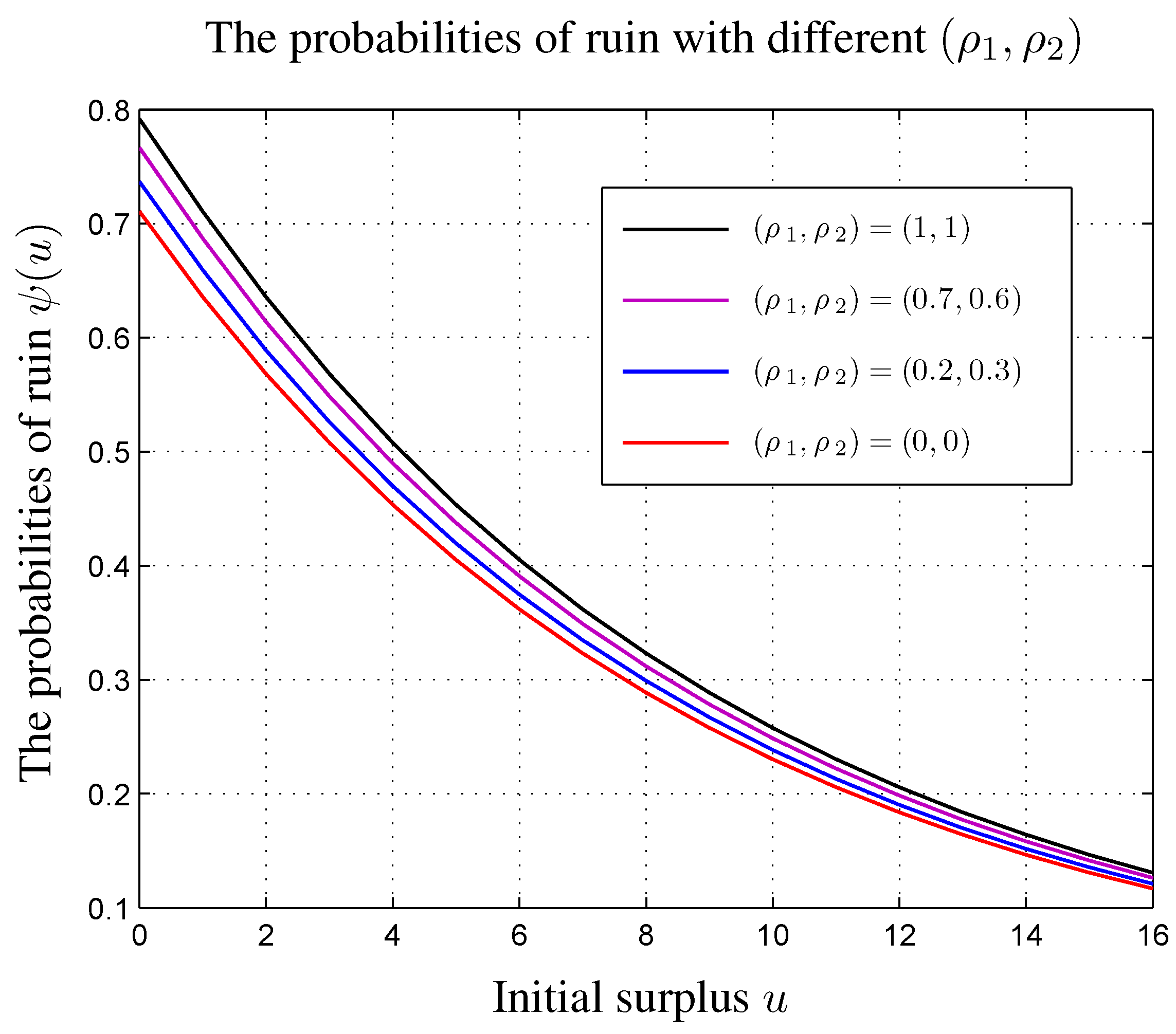
Example 2. We now revisit the example in Section 4.1. Suppose X and Y are both geometric distributed with ${\mu }_X=\frac{1}{1-a}$ and ${\mu }_Y=\frac{1}{1-b}$, respectively. The corresponding numerical results for $\psi \left(u\right)$ are shown in Figure 1 with $p_1=0.1$, $p_2=0.2$, $a=1/3$ and $b=1/4$.

Figure 1. The values of $\psi \left(u\right)$ with $p_1=0.1,p_2=0.2,a=1/3$ and $b=1/4$.

Figure 1. The values of $\psi \left(u\right)$ with $p_1=0.1,p_2=0.2,a=1/3$ and $b=1/4$.

5. Concluding Remarks

We study a discrete-time interaction risk model with delayed claims, which can be regarded as an extension to the prior work on time-correlated claims studied by [1,7]. Some analytic techniques are applied to study the expected discounted penalty function. We show that the expected discounted penalty function satisfies not only a recursive equation, but also a defective renewal equation. The results obtained in the present paper include the corresponding results in [7].

The model in this paper can be further extended. For instance, suppose that the dividend payments are ruled by a constant barrier in the framework of this paper; then, the calculation of the expected discounted dividend payments is necessarily possible.

References

- K.C. Yuen, and J. Guo. “Ruin probabilities for time-correlated claims in the compound binomial model.” Insur. Math. Econ. 29 (2001): 47–57. [Google Scholar] [CrossRef]
- H. Albrecher, and O. Boxma. “A ruin model with dependence between claim sizes and claim intervals.” Insur. Math. Econ. 35 (2004): 245–254. [Google Scholar] [CrossRef]
- E. Marceau. “On the discrete-time compound renewal risk model with dependence.” Insur. Math. Econ. 44 (2009): 245–259. [Google Scholar] [CrossRef]
- H. Cossette, E. Marceau, and F. Marri. “Analysis of ruin measures for the classical compound Poisson risk model with dependence.” Scand. Actuar. J. 2010 (2010): 221–245. [Google Scholar] [CrossRef]
- J.K. Woo. “A generalized penalty function for a class of discrete renewal processes.” Scand. Actuar. J. 2012 (2012): 130–152. [Google Scholar] [CrossRef]
- Z. Zhang, H. Yang, and H. Yang. “On a Sparre Andersen risk model with time-dependent claim sizes and jump-diffusion perturbation.” Methodol. Comput. Appl. Probab. 14 (2012): 973–995. [Google Scholar] [CrossRef]
- Y. Xiao, and J. Guo. “The compound binomial risk model with time-correlated claims.” Insur. Math. Econ. 41 (2007): 124–133. [Google Scholar] [CrossRef]
- Z. Bao, and H. Liu. “The compound binomial risk model with delayed claims and random income.” Math. Comput. Model. 55 (2012): 1315–1323. [Google Scholar] [CrossRef]
- X. Wu, and S. Li. “On a discrete time risk model with time-delayed claims and a constant dividend barrier.” Insur. Mark. Co. Anal. Actuar. Comput. 3 (2012): 50–57. [Google Scholar]
- R.S. Ambagaspitiya. “On the distribution of a sum of correlated aggregate claims.” Insur. Math. Econ. 23 (1998): 15–19. [Google Scholar] [CrossRef]
- R.S. Ambagaspitiya. “On the distributions of two classes of correlated aggregate claims.” Insur. Math. Econ. 24 (1999): 301–308. [Google Scholar] [CrossRef]
- H. Cossette, and E. Marceau. “The discrete-time risk model with correlated classes of business.” Insur. Math. Econ. 26 (2000): 133–149. [Google Scholar] [CrossRef]
- S. Li, and J. Garrido. “Ruin probabilities for two classes of risk processes.” Astin Bull. 35 (2005): 61–77. [Google Scholar] [CrossRef]
- S. Chadjiconstantinidis, and A.D. Papaioannou. “Analysis of the Gerber-Shiu function and dividend barrier problems for a risk process with two classes of claims.” Insur. Math. Econ. 45 (2009): 470–484. [Google Scholar] [CrossRef]
- L. Ji, and C. Zhang. “The Gerber-Shiu penalty functions for two classes of renewal risk processes.” J. Comput. Appl. Math. 233 (2010): 2575–2589. [Google Scholar] [CrossRef]
- X. Wu, and K.C. Yuen. “On an Interaction Risk Model with Delayed Claims.” In Proceedings of The 35th Astin Colloquium, Bergen, Norway, 6–9 June 2004; Volume 17.
- P. Brémaud. “An insensitivity property of Lundberg’s estimate for delayed claims.” J. Appl. Probab. 37 (2000): 914–917. [Google Scholar] [CrossRef]
- J. Trufin, H. Albrecher, and M. Denuit. “Ruin problems under IBNR dynamics.” Appl. Stoch. Models Bus. Ind. 27 (2011): 619–632. [Google Scholar] [CrossRef]
- A. Dassios, and H. Zhao. “A risk model with delayed claims.” J. Appl. Probab. 50 (2013): 686–702. [Google Scholar] [CrossRef]
- T. Rolski, H. Schmidli, V. Schmidt, and J.L. Teugels. Stochastic Processes for Insurance and Finance. Chichester, UK: Wiley, 1999, pp. 167–176. [Google Scholar]
© 2015 by the authors; licensee MDPI, Basel, Switzerland. This article is an open access article distributed under the terms and conditions of the Creative Commons Attribution license (http://creativecommons.org/licenses/by/4.0/).