1. Introduction
Electricity grids are in transition from fossil-based towards a low-carbon scenario, primarily based on renewable generation. This concept has led to the evolution of electrical grids to smart grids, dominantly focused on incorporation of renewable energy sources (RESs) into the electrical distribution grid and the ability to enable charging of an arbitrary number of electrical vehicles. This is a significant transition from traditional electrical (power) systems in which electricity demand was met by fossil-based bulk generated energy and conveyed to loads through transmission and distribution grids. The smart grid concept requires continuous development of power grids, at the transmission and distribution levels, developing new technologies and techniques as well as repurposing the existing ones.
Transmission grids remain vital also in the smart grids due to numerous reasons such as to convey energy from large renewable generation locations to demand sites, to link national markets and allow transfer of renewable electricity surpluses, and to support intermittent renewable generation to operate more efficiently. The task is to ensure the power flow by maintaining grid stability at the required power quality levels. As investments are very high, great attention is devoted to monitoring and maintaining the transmission lines.
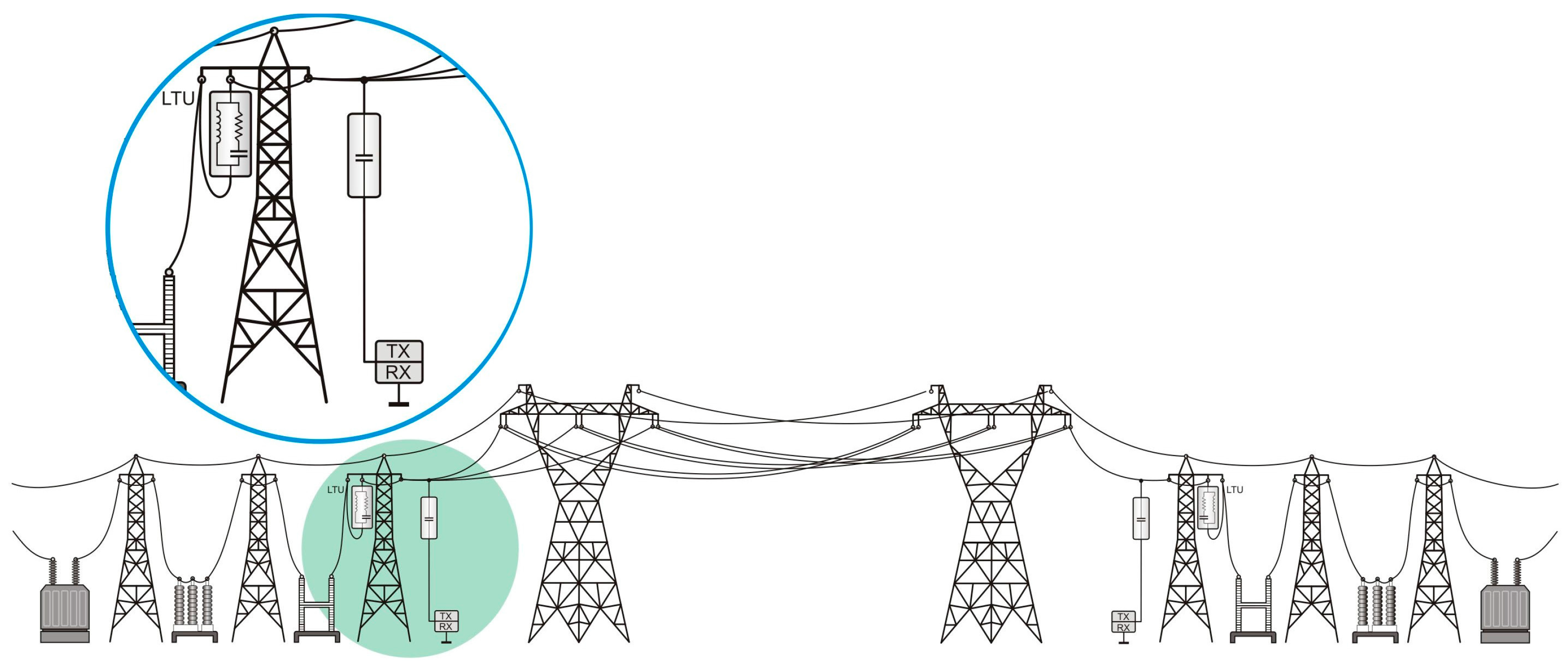
A transmission grid consists of high-voltage (HV) power lines spread over a large geographic area. In alternating current (AC) grids, electricity is transferred as three-phase voltages and currents at 50/60 Hz, which is usually denoted as the power frequency. Besides electricity transfer, HV power lines have also being utilized for communication purposes to transfer relevant operational data and protection signals (
Figure 1). With this aim, high-frequency (HF) signals can be injected into power line conductors at one terminal using appropriate frequency-selective circuits (filters) and extracted at the other terminal, not interfering with power-frequency “signals”. Information is superimposed into HF signals using analog or digital modulation.
This telecommunication technology founded on the HF signal transmission over HV power lines is known as power line carrier (PLC). Nowadays HV PLC doesn’t provide throughput that can compete with optical fiber or fourth generation (4G) cellular systems, and its application is very limited to specific applications in power systems. On the other hand, knowledge gained in the domain of HF signal transmission over HV power lines and the phenomena accompanying it can be used for some other advanced applications such as fault detection and localization. Mathematical models primarily derived for PLC communications are fundamental for the design of such advanced systems. Technology deployed in smart transmission grids can utilize these data as input for real-time monitoring of overhead power lines.
Electrical grids are facing the incorporation of intermittent renewable energy resources and the necessity for infrastructure reinforcement [
1]. Transmission system operators (TSOs) consider different power-line monitoring technologies to enhance operational efficiency of the existing HV power lines, such as Dynamic Line Rating (DLR) [
2,
3]. DLR is a sensor-based system that increases the transmission capacity by utilizing real-time data and information. These data include various factors that impact temperature of overhead conductors. With such an approach, the power line transmission capacity can reach 110–130% of the designed limits, under suitable weather conditions. Besides DLR sensors, information about the temperature of overhead power line conductors can be extracted from knowledge about overhead line catenary. In particular, power line sag is directly related to the weather conditions and temperature of conductors. In [
4], the authors proposed the application of PLC signals for real-time sag monitoring of HV overhead power lines. The method determines the average overhead conductor height variations in real-time, correlating mathematical models with the processed PLC signals captured at power-line terminals.
Ice load can cause severe damage on overhead power lines. The number of icing disasters on overhead power lines is increasing due to prevailing macroclimate, micrometeorological, and microtopography conditions [
5]. There are several complex methods to obtain information about the state of ice accretion based on real-time measurements with specific sensor systems [
6]. Another approach for icing thickness monitoring is based on image recognition algorithms [
5]. Ice load on overhead line conductors causes PLC signal propagation changes, which can be utilized for the detection of ice loads [
7]. In other words, ice load detection can be implemented through processing of PLC signals propagated over the HV power line.
Detection and classification of faults on HV power lines is crucial for stable and reliable power system operation. Various methods for detection, classification and location of faults on HV power lines have been studied, taking advantage of digital signal processing algorithms and machine learning methods [
8]. The common characteristic of all available approaches is to utilize measured phase voltage and current signals or fault-generated transient phenomena [
9,
10]. On the other hand, faults on power lines have a significant impact on frequency response. If a signal at PLC frequency is constantly injected, faults can be classified and located by processing the received signal at the line terminal. The authors of [
11] proposed a concept in which faults in multiconductor overhead distribution networks are detected using PLC devices. The method is based on detecting differences between values of metrics related to the input impedance at frequencies utilized by the PLC systems.
The purpose of this work is to provide the high-frequency model of faulted HV power line, which can be utilized for fault classification and localization purposes. This information is needed for future utilization of HV power lines for transmission of HF signals for various smart grid services. Analytical model is derived for the HV system under normal operation and evaluated with computer simulations validated with real HV power line measurements. This model is further extended for a faulted HV power-line and frequency response is obtained with computer simulations for different types of faults and deployed couplings. Different couplings are considered in order to determine the coupling with H(f) most sensitive to power-line faults.
The research presented in the paper is focused on high-frequency characteristics of HV power line under faulted operation. The main contributions of the paper are:
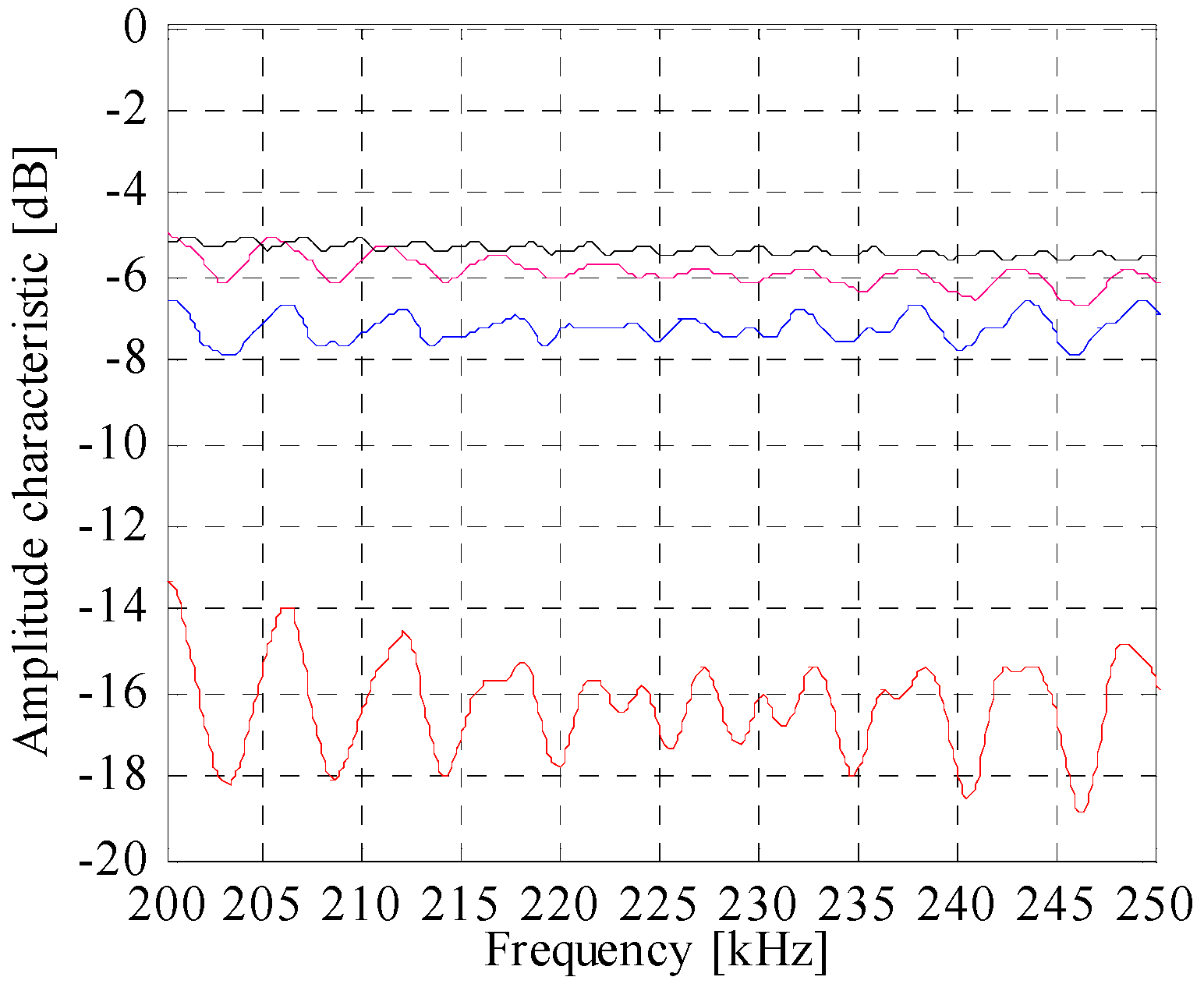
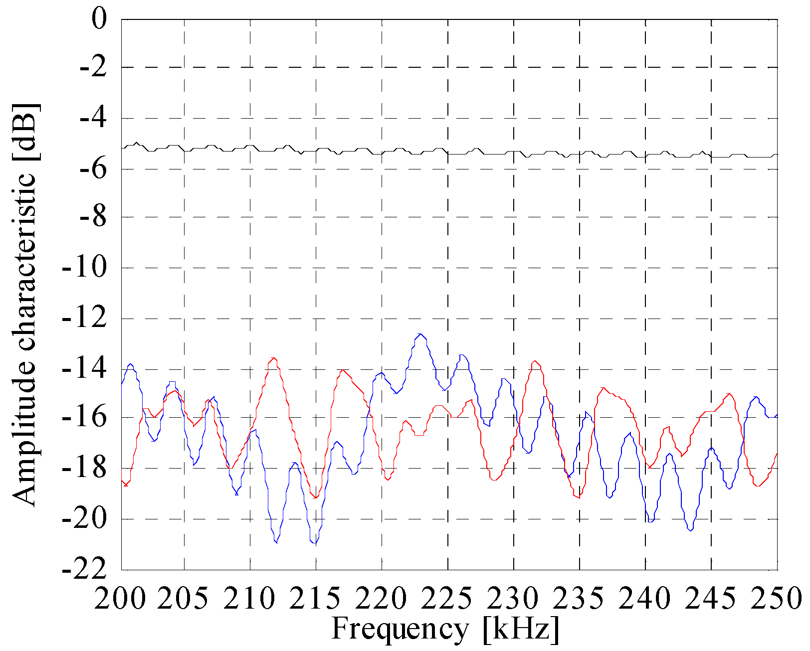
Telegrapher’s equations for multiconductor lines are extended with equations that provide characteristics for available couplings connecting electronic equipment to HV power-line conductors. This approach has been validated with actual measurements on 400 kV power line and outer-to-middle phase coupling.
The methodology for calculation of high-frequency characteristics of faulted HV power lines is developed for the series and shunt faults. The presented methodology is based on the validated approach used for HV power line in normal operation.
2. From HV PLC Systems to Advanced Power-Line Monitoring Applications
Reliable communications are fundamental component of modern power grids. The ability to utilize power lines for communications has attracted the research community for almost a century. At the transmission level, PLC presents one of the first communication technologies inside power systems. The range and quality of HV PLC communications strongly depends on the communication characteristics of the power lines (attenuation and noise), but also interference with other systems. HV overhead power lines radiate energy at high frequencies and interfere with other systems operating at the same frequencies. In Europe, the frequency range devoted to HV PLC system is from 30 kHz to 500 kHz [
12,
13,
14]. HV PLC systems are not permitted to operate in the broadband, but rather in the frequency range which is a multiple of 4 kHz bands to limit the interference. Therefore, HV PLC systems operate in a narrowband at carrier frequencies, which are determined at the deployment site to prevent interference. Available data rates are low for this reason, even at high spectral efficient digital modulation techniques (number of bits per Hz that channel transfers). On the other side, the major advantages of HV PLC communications are high reliability of these systems and the capability to transfer information over long distances, both crucial inside the smart grid concept.
HV PLC channels are characterized with very low attenuation, therefore communication signals can be transferred over very long distances. The distance is limited by the noise, generated by corona phenomena (discharges generated by rated high voltage) and interfering signals [
12,
13,
14]. Even though corona noise intensity varies with power frequency voltage, it doesn’t make huge impact on ultra-narrow band systems. It means that ultra-narrow band communication signals can be reliably used for control and command signals, such as trip signal for distant protection of HV power lines. Consequently, for decades HV PLC systems have provided a communication link to reach different power system components for control reasons and applications that require high reliability, low delays, and small throughput.
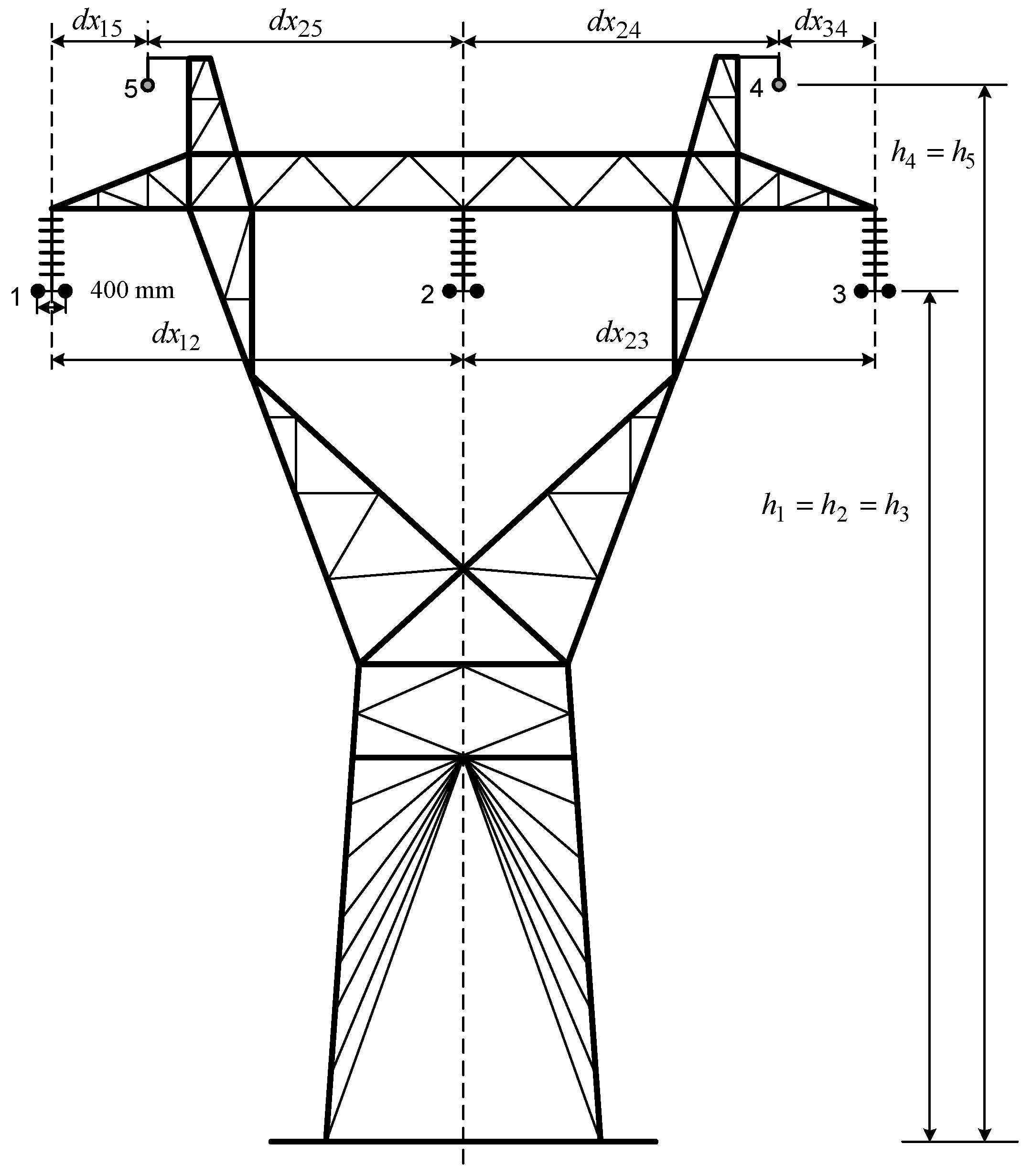
HV power lines employ three phase conductors (usually denoted as A, B and C) for electricity transfer and two shield wires for lightning protection. Schemes that describe how two terminals of communication equipment are connected to phase conductors are known as couplings. Shield wires are grounded at each power-line pole and cannot be used for signal transmission.
Coupling equipment blocks power-frequency voltages and forwards HF communication signals. Communication signals are blocked from propagating towards transformers at both power-line terminals by frequency-tuned circuits named line trap units (LTUs). PLC channel characteristics are different for individual couplings schemes. High-frequency signal transmission over the three phase conductors is coupled therefore the three phase conductors cannot be analyzed as three independent channels. For this reason, modal analysis is used to decouple PLC channel into three virtual modal channels. While modal channels are characterized with different attenuations, their excitation is directly correlated with the selected coupling scheme [
12,
13,
14].
For advanced HV power-line monitoring applications, a similar topology is used for HF signal injection and detection (
Figure 2). Each individual application defines the shape and frequency content of injected HF signals at the transmitting site as well as processing algorithms of captured signals at the receiving site. The condition of HV power line is superimposed into its frequency response
H(
f). Complete understanding of
H(
f) is crucial for design of advanced power-line monitoring applications utilizing HF signal propagation.
3. High-Voltage Overhead Power Line High Frequency Characteristics in Normal Operation
Voltage and current propagation along a transmission line can be described with telegrapher’s equations. Since HV power line is a multiconductor line, telegrapher’s equations take a matrix form. Telegrapher’s equations in the matrix form are derived from Maxwell equations and can be simplified for the case of sinusoidal voltages and currents [
15,
16].
In order to obtain frequency response of a HV power line, we consider propagation of time-harmonic voltages and currents along the power line. Our analysis uses two assumptions:
HV power line is a linear system.
Only stationary states are considered.
Transmission line is assumed to be infinitely long.
Telegrapher’s equations for the case of sinusoidal voltages and currents are derived starting with the equivalent electrical scheme of infinitely small line lumps [
17].
3.1. Wave Propagation on Infinetely Long Homogoneous Multiconductor Transmission Line
In order to describe wave propagation over a multiconductor transmission line, we use the equivalent electrical circuit of a line lump [
17]. In the first step, the transmission line with one cylindrical conductor parallel with the earth plane and harmonic sources at the line terminals are considered.
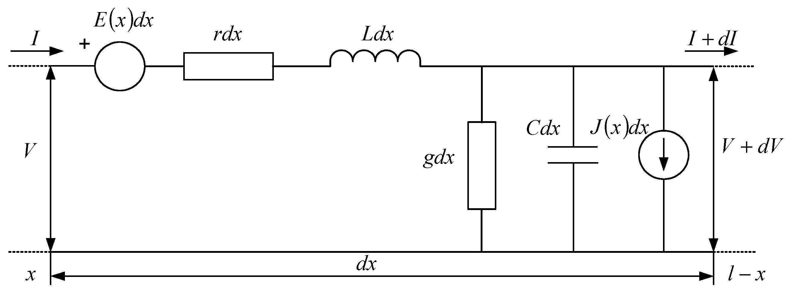
Voltage and current at any arbitrary point on the line are determined with concentrated harmonic sources at the line terminal as well as distributed sources along the line, together with the transmission line characteristics. This is modelled with an equivalent electrical circuit of line lump with concentrated parameters as is shown in
Figure 2 [
17].
Distributed voltage and current sources exist due to different types of noise (e.g., Corona noise) appearing on the transmission line. The line is characterized with passive elements per unit length: r, L, g and C. Element r corresponds to the line resistance per unit length while L is the inductance per unit length. The shunt passive elements g and C represent a conductance and a capacitance of transmission line per unit length.
The analysis is reduced to harmonic voltage and current propagation, presented as phasors rotating with angular frequency
f. According to
Figure 2, the increment of the voltage and current across the line lump can be written as [
17]:
where
is the line impedance per unit length and
is the shunt admittance per unit length. Separating variables in the coupled Equation (1) and neglecting the term
dV in comparison with
V, equations describing voltage and current along the transmission line are obtained:
These equations are also known as telegrapher’s equations for the transmission line with a single conductor above the ground. Equation (2) can be extended to the multiconductor case. A major difference with the previous case is the existence of magnetic and electrostatic couplings between the conductors. The magnetic coupling is modeled with the distributed voltage sources per unit length Eij and Eji, and mutual impedances zij = zji. Electrostatic coupling is represented with admittance yij between the conductors.
A number of equations increases with a number of conductors and therefore it is appropriate to write Equation (2) in a matrix form [
16,
17]:
where
Z and
Y are square matrices:
and
n is the number of conductors. Vectors
V,
I,
E and
J have all dimension
n × 1.
Variable separation in Equation (3) derives matrix telegrapher’s equations:
In the case of a passive network, distributed sources are equal to zero and the telegrapher’s equations become:
Matrices
Z and
Y in Equation (3), also found in the literature as primary parameters of a transmission line, define how the harmonic voltage and current propagate over a multiconductor transmission line. The detailed calculation of the HV overhead power line primary parameters is given in [
12,
13,
14].
3.2. Solution of the Telegrapher's Equations
The non-diagonal elements of matrices
Z and
Y, corresponding to couplings between the phases, make solution of telegrapher’s equations difficult. Therefore, let’s replace the product of matrices
Z and
Y with the matrix
taking into account that matrices
Z and
Y are symmetrical [
17]:
furthermore:
In analogy with the propagation constant, we will denote this matrix as the propagation matrix. Equation (6) can be rewritten as:
In case that
is a diagonal matrix, the previous equation is equal to the set of
n independent differential equations. Therefore, we need to find an appropriate linear transformation that results in the diagonal matrix
. This linear transformation is founded on matrices
S and
Q, correlating voltages and currents in natural (phase) coordinates
V and
I with voltages and currents in modal coordinates
and
[
16,
17,
18]:
Substituting the expression for the voltage and current vectors defined with Equation (10), Equation (9) becomes:
The matrix
S is determined to diagonalize the product [
18,
19]:
We conclude that elements of the diagonal matrix
γ2 are eigenvalues of the matrix
, where columns of the matrix
S are their corresponding eigenvectors [
18,
20,
21].
Matrices
ZY and
YZ are similar since:
and therefore the product
YZ has the same eigenvalues [
18,
19,
20]. The columns of the matrix
Q are eigenvectors of the matrix
, resulting in:
The presented analysis that decouples telegrapher’s equations into 2 ×
n ordinary differential equations is known as modal analysis. The modal analysis introduces decoupled modal channels. Propagation of a modal voltage and current through the modal channel
k is described by a modal propagation constant
. The modal voltage and current in the modal channel
k at the arbitrary point
x can be expressed as:
Constants
and
are calculated using boundary conditions at the power-line terminal. A column vector of the matrix
S defines distribution of the modal voltage between the phase conductors. Distribution between the power-line conductors
i and
j is defined with the ratio:
Matrix
S is usually normalized with respect to the first row that is multiplied with a transformation matrix in the manner that elements in the first row are all equal to one. We denote such normalized matrix
S with
λ. Similar expressions can be derived for currents:
where matrix
Q is normalized in respect to the first row, denoted with
.
3.3. Characteristic Impedance Matrix
Voltage
and current
propagate through the modal channel
k independently from other modal channels. At an arbitrary point
x on a power line, the modal voltage and current are equal to the sum of incident and reflected waves, as it is written in Equation (15). The modal characteristic impedance establishes a relation between the modal incident voltage and current with modal reflected voltage and current:
for
k = 1,…
n, or rewritten in a matrix form:
where
is a diagonal matrix containing characteristic impedances of modal channels:
Matrix
is a diagonal matrix defined as:
Modal voltages at an arbitrary point
x equal to the sum of incident and reflected waves:
while corresponding modal currents are:
The boundary condition at the first line terminal determines constants
and
. Substituting the modal voltage in modal telegrapher’s Equation (11) with equations (22) and (23), modal characteristic impedance [
17] is derived:
The modal characteristic admittance matrix is defined by:
Voltage and current vectors in natural (phase) coordinates are computed from modal voltage and current vectors obtained as a solution of the telegrapher’s equation. Equations (10) and (19) also correlate incident and reflected waves in natural coordinates with incident and reflected waves in the modal coordinates:
where
and
are the incident voltage and current vectors in natural coordinates. Characteristic impedance matrix
is computed as:
while the characteristic admittance matrix is:
Substitution of the modal voltage and current in Equation (10) with Equations (24) and (25) yields [
19]:
We introduce the exponential function:
and denote:
then Equation (29) can be rewritten in the form:
Vectors
and
are computed from boundary conditions defined at the power-line terminal. When boundary conditions are
and
, vectors
and
are found to be:
Substitution of previous expressions into Equation (32) yields [
17]:
3.4. Characteristics of HV Power Line Terminated with Impedance
Communication equipment can be connected to a HV power line in different couplings (to one, two or three phase conductors), employing different power-line channels for data transmission. Each power-line channel is characterized with its own frequency-dependent transfer function since different couplings excite different modes.
There are two major approaches to HV power-line modeling based on the modal analysis [
16]. The first approach utilizes the power-line multiport representation and reduction of ports in respect to the used coupling, without computation of voltages and currents. The second approach computes received voltages and currents with known transmitted voltages and currents for the selected coupling. This approach incorporates the reflection coefficient and it is usually denoted as a method of matrix reflection coefficients [
7,
17,
21].
If
and
are known harmonic voltage and current of an arbitrary frequency
f at the power-line transmitting end and
and
are received voltages at the other line end, the frequency-dependent power-line transfer function is defined with the amplitude
and phase characteristic
β:
where:
3.4.1. Voltage Transfer Matrix
The voltage and current at the transmitting line terminal are interrelated through the input admittance (or input impedance) matrix and at the receiving end with the load admittance matrix:
The voltage and current at the line terminal is a sum of incident and reflected components:
Solving the set of Equation (38) per incident and reflected voltages, and taking into account Equation (37), yields:
A reflection coefficient represents a ratio between the reflected and incident waves. Since a power line is a multiconductor system, the reflection coefficient is a square matrix correlating the reflected and incident waves at different ports:
Utilizing Equations (39) and (40), the matrix reflection coefficient at the receiving terminal is:
Similarly, the voltage at the transmitting line terminal is expressed in terms of the incident wave and matrix reflection coefficient
[
7]:
Since the incident voltage at the receiving line end is determined by the propagation function and the power-line length:
the voltages at the receiving and sending line ends are interrelated with:
where matrix
T is the voltage transfer matrix.
The matrix reflection coefficient is obtained by interrelating reflected and incident waves at the transmitting line terminal [
16,
22]:
while the input admittance is:
If a reflection is considered in the modal coordinates, we deal with the modal incident and reflected waves are interrelated with the modal reflection coefficient. The relation between the incident and reflected waves in phase (original) and modal coordinates is established with:
where index
x is used to denote both line ends. The modal reflection coefficient is then derived from Equations (40) and (47):
The transformation defined by Equation (48) results in a non-diagonal matrix, what causes power exchange between modes at the termination points. A conclusion is that modal waves propagate along the modal channels without interacting between each other. However, interaction occurs at the termination points. On the other hand, any inhomogeneity on a power line produces reflected waves and power exchange between modes.
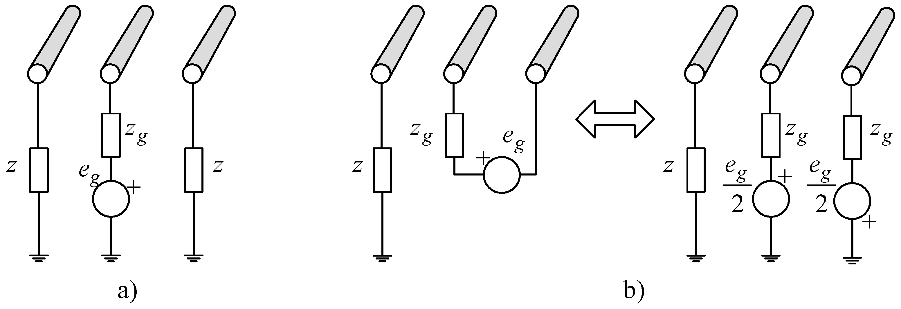
3.4.2. Computation of High-Frequency Power-Line Transfer Function for Different Couplings
In this section we focus on two types of coupling utilizing one or two phase conductors, presented in
Figure 3.
Voltages at the transmitting and receiving ends of a HV power line are correlated with voltage transfer matrix T. Corresponding currents are calculated using termination admittances at both power-line ends, denoted with matrices and .
When the voltage transfer matrix is determined, high-frequency power-line channel characteristics for different couplings can be obtained with two approaches:
The first is to assume a value of the source (voltage or current) and to compute voltages and currents at both line terminals. High-frequency power-line channel characteristics are then computed from the Equation (36). In case of very long lines, such approach can cause a significant numerical inaccuracy that increases with the frequency.
In the second approach, the high-frequency power-line characteristics are computed directly from the voltage transfer matrix, utilizing information of relations between the voltages at the both line ends contained in the matrix T.
A problem that arises in such formulae derivations is related to a multiconductor system, where voltages of all output ports are interrelated with all voltages of all input ports. In the first step, frequency response is calculated for the phase to ground coupling. We suppose that the transmitter is modeled as the voltage generator
and impedance
. Since the voltage source impedance is
zg, the expression that defines voltages of the three phases at the transmitting line terminal is:
Let’s consider a transmitter connected between the phase
k and the ground and a receiver between the phase
t and the ground, as presented in
Figure 3a. The amplitude and phase characteristics are computed as:
The
k-th element in the vector
equals
, while other elements are zero. Equation (49) simplifies to:
where
is
k-th column of the matrix
L. In the next step all phase voltages should be expressed in term of one parameter. For instance, voltage of the first port
at the sending end can be chosen as such parameter. The ratio between the voltage of the phase
i and the voltage of phase 1 is:
vector
contains elements defined by Equation (53). Now, vector
is expressed in the term of
Further we rewrite the voltage at the receiving end in the term of parameter
V1(1):
and the voltage of the phase
t at the receiving end is found to be:
where
is a row
t of the matrix
T. The current at the sending end equals to:
where
F is the auxiliary square matrix. If with
we denote row
k in the input admittance matrix
and with
row
t in the matrix
F, then the voltage of phase
k at the sending end and the voltage of the phase
t at the receiving end equal to:
Substituting the expressions for the both line ends in Equation (51) we derive:
Equation (59) defines the high-frequency power-line channel characteristics for the phase to ground coupling. A similar analysis can be conducted also for phase to phase coupling (
Figure 3b). Let’s assume the coupling phase
j to phase
k at the transmitting power-line terminal and phase
s to phase
t at the receiving terminal. The elements of the voltage vector
equal zero, except
s-th and
k-th elements that are:
If
and
denote
j-th and
k-th columns of the matrix
L respectively, the voltage at the sending terminal is:
Likewise, the phase to ground coupling, elements of the voltage vector
are expressed in the term of voltage
utilizing the vector column
whose elements are:
The voltage at the transmitting end is then:
and for the selected coupling:
Voltage at the receiving end is correlated to the voltage at the sending end with the voltage transfer matrix:
and the voltage at the receiver is:
The currents at the power line terminals are:
When
represents the
j-th row of matrix
Yin and
Fs corresponds to the
s-th row of the matrix
B, currents at the receiver and at the transmitter respectively are:
The high-frequency power-line channel characteristics are then derived from Equations (64), (66) and (68) as:
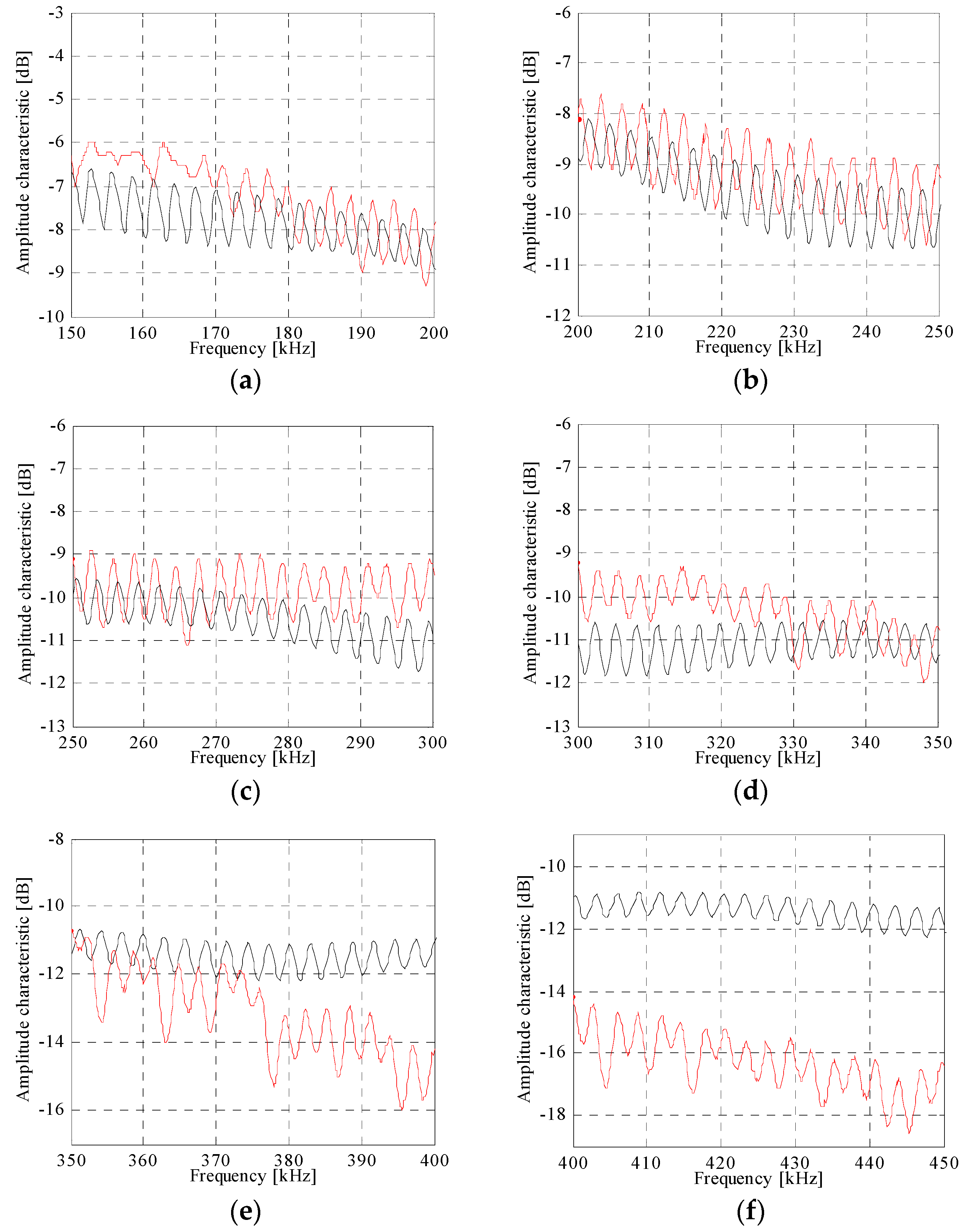
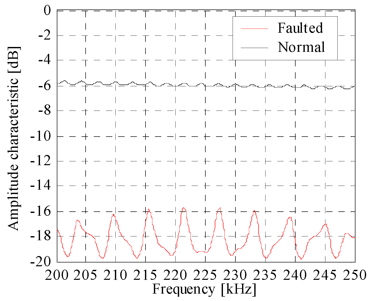
4. High-Frequency Characteristics of Faulted HV Overhead Power Line
In this section we analyze high-frequency response of HV power line under different fault conditions. For this purpose we start with previously derived model of a HV power line in normal operation, validated with actual measurements. Faulted HV power line model is derived for all known HV power line faults, which are divided into two categories [
23,
24]:
shunt faults,
series faults.
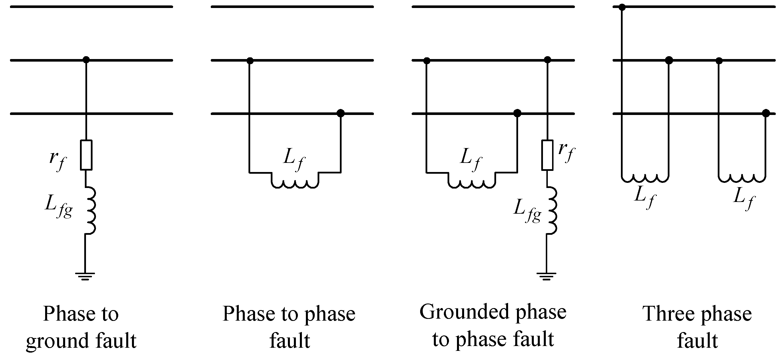
The shunt faults refer to all types of short circuits that are further categorized as [
25]:
short circuit between one phase and the ground (phase to ground fault),
short circuit between two phases, with possibility of simultaneous grounding (phase to phase fault and grounded phase to phase fault),
short circuit of all three phases (three phase fault).
Short circuits are also denoted as permanent or temporary, depending on whether they still exists when power line is not rated by a high voltage. The permanent faults are caused by breaking phase or shielding conductors and short circuiting with the other phase conductors or the ground. The temporary short circuits exist due to arcs and disappear after the power line is switched off. Temporary faults can be initiated by the temporary insulation breakdown due to short-duration atmospheric discharges. Since a large amount of faults are “self-healing”, the automatic reclosure process is utilized instead of permanent power-line switch off. Automatic reclosure attempts to switch on the power line until the short-circuit path is deionized. After the predefined number of unsuccessful attempts (usually up to three times) the power line remains switched off [
26].
The series faults correspond to a phase conductors breaking without connection with other phase conductors or the ground. Together, the series and shunt faults on the two sides of the fault location on the power line form the hybrid type fault. The most common faults are phase to ground faults. They contribute three quarters of all faults while the rarest are the three phase faults [
27].
Next we derive the method to compute characteristics of the faulted power line. It should be noticed that short circuits are always followed by the power line trip in order to prevent the severe damage of the equipment due to high short-circuit currents. In the analysis we assume that tripped power line is terminated with modified impedances what causes changed high-frequency characteristics.
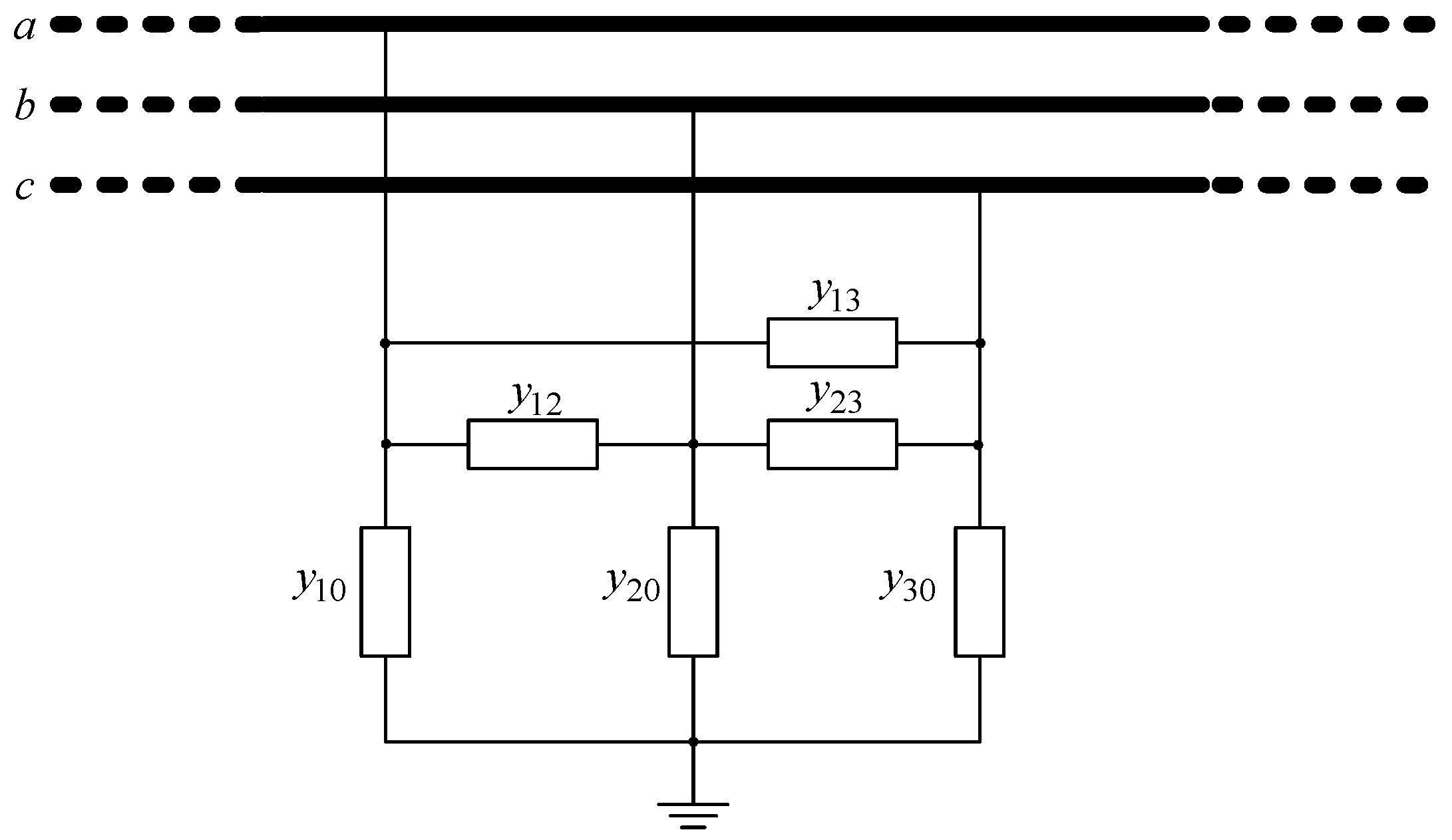
4.1. Fault Modeling with Shunt Impedance
The shunt impedance on the HV power line is defined as an electrical system that consist of passive elements connected between power-line (phase or shield) conductors and the ground or between power-line conductors only (
Figure 4). Inhomogeneity (fault location) is modelled with a shunt admittance matrix
Ysh.
There are two approaches to incorporate the shunt impedance in the derived high-frequency power-line model. The first approach utilized the method of the matrix reflection coefficients in compliance with the previous section. It is obvious that a reflected wave appears at the shunt point where the impedance changes. This phenomenon is incorporated in the analysis with the matrix reflection coefficient computed as [
27]:
where
is the admittance matrix terminating the line section before inhomogeneity and equals:
The admittance matrix Yin2 is the input admittance of the second line section.
4.2. Short Circuits
A short circuit represents a fault when a power line conductor forms an electrical contact with another conductor or the ground through some impedance. Such fault is therefore represented by the shunt impedance at the fault location. The faulted power-line high-frequency characteristics are then obtained as described in
Section 4.1.
The fault analysis is often conducted with an assumption that a fault impedance equals zero. It implies that the power-line channel attenuation with the phase to phase coupling tends to infinity when grounded phase to phase fault or three phase fault occurs. However, it can be found in the literature that attenuation introduced by a short circuit doesn’t overreach 40 dB to 50 dB and that reduces with frequency [
7]. A magnetic coupling between two line sections separated by the fault can be represented as inductive reactance connected at the fault location. The expressions that define the fault impedances for different couplings are available in [
7,
17,
27].
The fault impedance between the phase conductor and the ground (for phase to ground fault) is computed as [
7,
27]:
where
is the sum of a grounding resistance (between 10 Ω and 20 Ω) and a conductor caused the short circuit (or arc). According to [
7,
27],
for phase to ground fault is computed as:
where
h and
are the length and radius of the grounding conductor. The previous expression holds when the distance to the fault from the coupling device is
[
7].
In the case of a phase to phase fault, without grounding, the fault impedance is computed as a short circuit between the two parallel lines. The resistance is neglected, while inductance equals to [
27]:
The grounded phase to phase fault is a combination of the above defined impedances. The short circuit is schematically represented in
Figure 5.
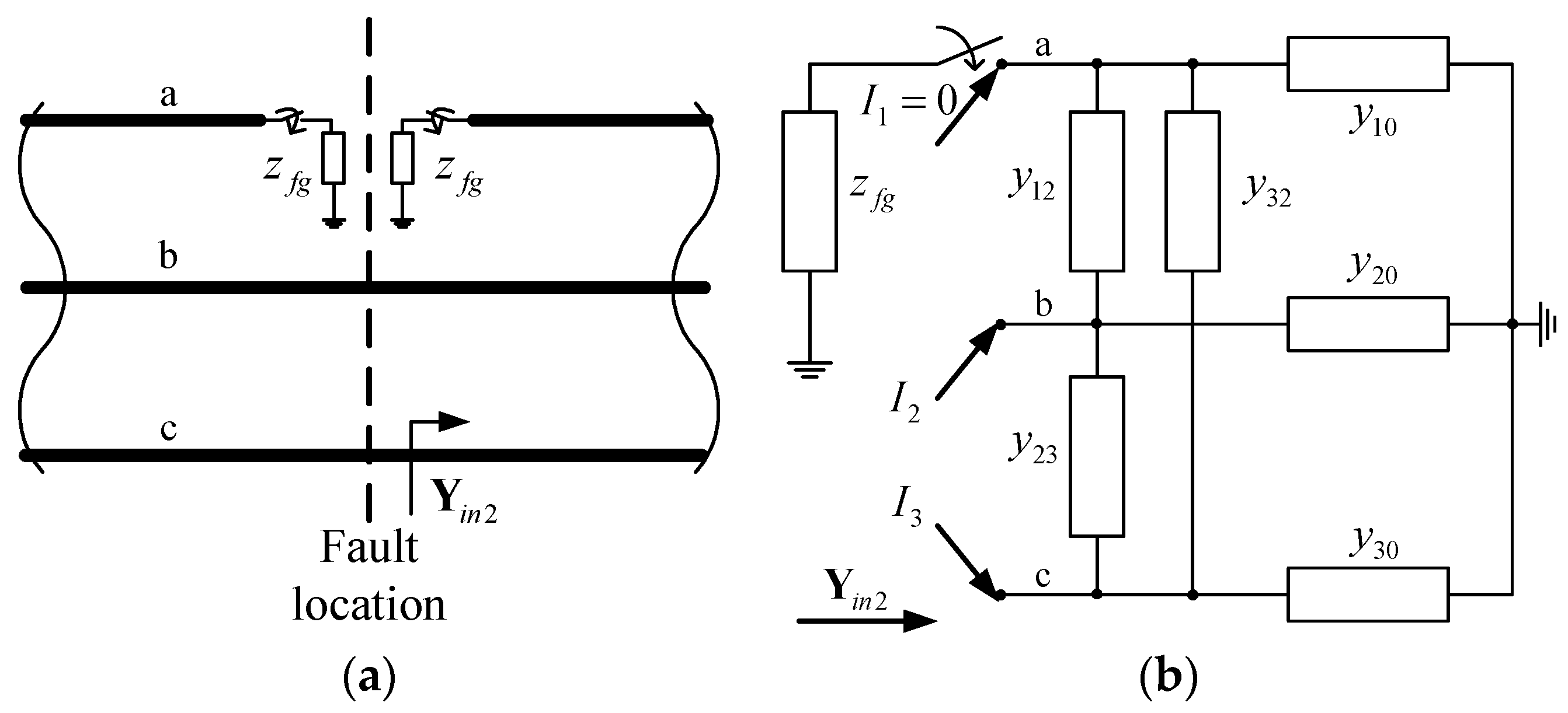
4.3. Series Faults
A series fault occurs when one of phase conductors breaks without any connection between phases or between a phase and ground [
23]. However, it is common that one of phases or both after the breaking fall down on the ground what causes a phase to ground fault. Such case is denoted as a hybrid fault. We consider one phase break, with possibility that a phase conductor at both sides can also be grounded (falling down on the ground), presented in
Figure 6.
A fault divides the line into two sections. In order to determine the admittance terminating the first line section, let’s assume that the fault occurs on the first phase conductor. We consider two options: phase conductor can be open-circuited or short-circuited via impedance
zfg. The impedance
zfg corresponds to the phase to ground impedance, computed in the previous sub-section. The input impedance of the second section
Yin2 is schematically represented in
Figure 6b and can be determined for the line termination admittance
. The interrelation between voltages and node currents on the right side of the fault location (
Figure 6) is established as:
where
,
and
are node currents. Admittance
is an element (
i,
j) of the matrix
while
or
. When the first phase conductor is faulted, the node current
equals zero and:
Substituting previous equation into Equation (75), a relation between the two other voltages and node currents can be written in the matrix form as:
It is obvious that the second and third phases of the first line section are terminated with the second line section while the first phase is either short-circuited via fault impedance or open-circuited. Therefore, the admittance terminating the first line section is:
If the termination admittance at the fault location is known then the first-section voltage transfer matrix
T1 is determined, and voltages at the sending line terminal and the left-side fault locations can be calculated:
When the line is terminated with the load admittance
, the second-section voltage transfer matrix is found in compliance with the analysis conducted in the previous sub-section. Voltage at the line end equals to:
where
is the voltage vector at the beginning of the second line section. Furthermore, the voltages at the both sides of the fault location are interrelated with the fault voltage transfer matrix:
where
is calculated taking into account Equation (77) as:
The voltage transfer matrix is:
Power-line high-frequency characteristic are computed from the equations derived in sub-
Section 3.4. Due to simplicity, the expressions are derived for the first phase while analogy is valid for the faults of the two other phases.


