From Theory to Econometrics to Energy Policy: Cautionary Tales for Policymaking Using Aggregate Production Functions

Abstract

Development of energy policy is often informed by economic considerations via aggregate production functions (APFs). We identify a theory-to-policy process involving APFs comprised of six steps: (1) selecting a theoretical energy-economy framework; (2) formulating modeling approaches; (3) econometrically fitting an APF to historical economic and energy data; (4) comparing and evaluating modeling approaches; (5) interpreting the economy; and (6) formulating energy and economic policy. We find that choices made in Steps 1–4 can lead to very different interpretations of the economy (Step 5) and policies (Step 6). To investigate these effects, we use empirical data (Portugal and UK) and the Constant Elasticity of Substitution (CES) APF to evaluate four modeling choices: (a) rejecting (or not) the cost-share principle; (b) including (or not) energy; (c) quality-adjusting (or not) factors of production; and (d) CES nesting structure. Thereafter, we discuss two revealing examples for which different upstream modeling choices lead to very different policies. In the first example, the $\left(kl\right)e$ nesting structure implies significant investment in energy, while other nesting structures suggest otherwise. In the second example, unadjusted factors of production suggest balanced investment in labor and energy, while quality-adjusting suggests significant investment in labor over energy. Divergent outcomes provide cautionary tales for policymakers: greater understanding of upstream modeling choices and their downstream implications is needed.

1. Introduction

Development of energy and economic policy is often informed by energy-economic modeling via aggregate production functions (APFs) fitted to historical data in a theory-to-policy process utilized in the literature [1,2], in government budget offices [3], and at the World Bank [4]. Although a theory-to-policy process could be constructed without the use of APFs, this paper focuses on the common practice of fitting APFs to historical time series data in the middle of the theory-to-policy process.

Despite more than 60 years of criticism [5,6,7], the use of APFs continues and appears to be expanding, with APFs moving from academic study [8,9] to macroeconomic modeling that informs energy and economic policy [10,11,12]. Empirical applications of APFs are numerous, including analysis of (a) technical change [13]; (b) substitution elasticities [14]; (c) inter-country economic output and structure [9,15]; and (d) CO${}_2$ emissions policy [16]. One reason for the enduring allure of APFs is their promise to describe the intricate, complex workings of entire economies by simple, aggregated measures of inputs (capital, labor, and sometimes energy) and output (typically, Gross Domestic Product, GDP).

The theory-to-policy process is not merely academic: the policies it generates affect economic development and quality of life for people worldwide. Furthermore, unsettled debates about the best way to account for energy in economic models lead to unclear policy prescriptions in the face of energy-related environmental challenges, including climate change. Like all modeling, fitting APFs to historical data is necessarily a simplification of the complex world in which we live. That simplification is fraught with potential perils, including the following circular truths: (a) our understanding of reality shapes the modeling approaches we employ and (b) modeling results affect our understanding of reality. Indeed, the theory-to-policy process highlights the fact that interpretation of economic data is often mediated by models on the way to establishing the energy and economic policies needed to address some of humanity’s most pressing challenges while improving human well-being (which is enabled by the availability of inexpensive energy). Therefore, it is essential that we, from time to time, step back to critically evaluate the theory-to-policy process, including APFs, estimation of their parameters, their role and use in the process, and the effects of upstream modeling choices on downstream policymaking. To date, few studies have done so, a gap which this paper attempts to fill.

2. The Theory-to-Policy Process

Aggregate production functions are a key aspect of the theory-to-policy process outlined in Section 2.2 below. So before providing details of the process, we summarize APFs.

2.1. Aggregate Production Functions (APFs)

APFs seek to describe economic output via factors of production, such as capital, labor, and energy. The origins of APFs can be traced to von Thünen in the 1840s [17,18], and the meaningfulness of models built using APFs has been debated nearly as long. Mishra [18] provides an excellent history of production functions and a detailed discussion of the key controversies surrounding their use. Brockway et al. [19] is a “sister” paper to this and provides a general, non-empirical discussion of the landscape around CES APFs, summarizing several notable critics and their arguments [5,6,20,21,22] and providing guidance for the application of the CES APF to economic growth modeling. Recent application of cointegration analysis by Santos et al. [23] suggests that APFs can provide statistically significant long-run relationships among economic output, capital, labor, and energy, thereby avoiding the critique of APFs in Felipe and Fisher [7]. The issues swirling around APFs are sometimes acknowledged by practitioners. For example, Miller [24] (p. 10) reviewed different APFs for use in the US Congressional Budget Office (CBO) model, and suggested that “even if our [CBO model] is misspecified and the parameters are in fact statistical artefacts, they may still be useful for forecasting purposes”. Our approach is (a) to acknowledge the widespread usage of APFs despite the various concerns and (b) to demonstrate empirically the effects of APF modeling choices through to policy.

We apply and evaluate APFs at the national level, although APFs can be used at the sectoral level, too. Many of the issues discussed here arise from the statistical estimation of APF parameters, and those issues will pertain to both national and sectoral levels.

Historically, the most common mainstream APF has been the Cobb-Douglas (C-D) function:

$$y=\theta {\mathrm{e}}^{\lambda t}{k}^{{\alpha }_k}{l}^{{\alpha }_l},$$

(1)

where economic output (y) is written as a function of the traditional factors of production capital (k) and labor (l). Greek letters in this and other APFs represent unknown parameters that must be estimated. When referring to parameter estimates, we add the Latin circumflex (e.g., $\widehat{\theta }$).

In the C-D APF, the parameters θ, ${\alpha }_k$, and ${\alpha }_l$ are, respectively, a scale parameter and output elasticities for capital and labor. Output elasticity is defined as the normalized partial derivative of economic output with respect to a factor of production, ${\alpha }_i\equiv \frac{\frac{\partial y}{\partial x_i}}{\frac{y}{x_i}}$. The constraint $\sum {\alpha }_i=1$ is often applied to impose constant returns to scale. (Under constant returns to scale, economic output increases by the same proportion as all inputs increase, all other things being equal. For increasing returns to scale, $\sum {\alpha }_i>1$ and output increases by a greater proportion than all inputs. For decreasing returns to scale, $\sum {\alpha }_i<1$.) The term $A\equiv {\mathrm{e}}^{\lambda t}$ is known as the Solow residual, here represented as an exponential with growth rate λ. (The Solow residual is a representation of exogenous factors that influence economic growth, and, as such, represents that part of economic growth not explained by endogenous factors of production. In the case of Equation (1), the endogenous factors of production are k and l. The Solow residual is often attributed to “technology”. In Equation (1), the Solow residual multiplies all endogenous factors of production and is sometimes called “total factor productivity”.) Solow’s study [8] of the US economy using Equation (1) “was a landmark in the development of growth accounting” [25] and started a burgeoning literature on the topic.

Equation (1) can be generalized in a natural way to include additional factors of production (e.g., energy, e):

$$y=\theta {\mathrm{e}}^{\lambda t}{k}^{{\alpha }_k}{l}^{{\alpha }_l}{e}^{{\alpha }_e}.$$

(2)

Disadvantages of the C-D APF are (a) output elasticities (α) that are constant through time and (b) elasticities of substitution (σ) that are fixed at 1. The Hicks elasticity of substitution between factors of production $x_1$ and $x_2$ is defined as ${\sigma }_{x_1,x_2}\equiv -\frac{\partial ln\left(\frac{x_1}{x_2}\right)}{\partial ln\left(\frac{\partial y/\partial x_2}{\partial y/\partial x_1}\right)}$ and quantifies the ease with which $x_1$ and $x_2$ can substitute for each other in an economy. (See Sorrell [26], Equation 24.) ${\sigma }_{x_1,x_2}=0$ indicates that $x_1$ and $x_2$ are perfect complements. ${\sigma }_{x_1,x_2}=\infty$ indicates that $x_1$ and $x_2$ are perfect substitutes. (See Sorrell [26] for discussion of and taxonomy for various elasticities of substitution.) The Constant Elasticity of Substitution (CES) APF [27] generalizes Equation (1) and addresses these drawbacks:

$$y=\theta {\mathrm{e}}^{\lambda t}{\left[{\delta }_1{k}^{-{\rho }_1}+(1-{\delta }_1)l^{-{\rho }_1}\right]}^{-1/{\rho }_1}.$$

(3)

In Equation (3), ${\delta }_1$ provides weighting for the factors of production, and the elasticity of substitution is easily accessible from model parameters: ${\sigma }_1=\frac{1}{1+{\rho }_1}$. Equation (3) assumes Hicks-neutral technical change ($A\equiv {\mathrm{e}}^{\lambda t}$ augments all factors of production), because, as Henningsen and Henningsen [28] (p. 25) note, a consensus approach to non-neutral technical change (wherein each factor of production has its own A) has not yet emerged. (See Frieling and Madlener [29] for an example of factor-specific technical change.) If ${\rho }_1=0$ (${\sigma }_1=1$), the CES APF (Equation (3)) simplifies to the C-D APF (Equation (1)).

Generalization to three factors of production can be accomplished by nesting two factors of production ($x_1$ and $x_2$) against the third ($x_3$):

$$y=\theta {\mathrm{e}}^{\lambda t}{\left\{\delta {\left[{\delta }_1{x}_1^{-{\rho }_1}+(1-{\delta }_1)x_2^{-{\rho }_1}\right]}^{\rho /{\rho }_1}+(1-\delta )x_3^{-\rho }\right\}}^{-1/\rho },$$

(4)

where $x_1$, $x_2$, and $x_3$ are permutations of the factors of production k, l, and e.

Table 1. Nesting structures for CES APFs.

Nesting Structure	${\mathit{x}}_1$	${\mathit{x}}_2$	${\mathit{x}}_3$
$kl$	k	l	0
$\left(kl\right)e$	k	l	e
$\left(le\right)k$	l	e	k
$\left(ek\right)l$	e	k	l

shows three of six nesting structures for Equation (4). The other three nesting structures [$\left(lk\right)e$, $\left(el\right)k$, and $\left(ke\right)l$] produce identical fits to historical data. Note that Equation (3) is a degenerate form of Equation (4) with $x_1=k$, $x_2=l$, $\delta =1$, and ρ undetermined.

Because output elasticity (Section 3.2) is unlikely to be constant over time and because the substitutability and complementarity of factors of production may vary from one economy to the next and from factor to factor within an economy, the CES APF is potentially better suited to describe economic output than the C-D APF. However, the increased suitability of the CES APF comes at a cost: with more parameters and a non-linear structure (in logarithmic space), the CES APF is more demanding than the C-D APF in terms of fitting technique, computational resources, and economic interpretation. The C-D APF (Equation (1)) has three free parameters (θ, λ, ${\alpha }_k$, with ${\alpha }_l=1-{\alpha }_k$ for constant returns to scale), and the CES APF (Equation (3)) has four free parameters (θ, λ, ${\delta }_1$, ${\rho }_1$).

Brockway et al. [19] found that the two most common APFs are C-D (Equation (1)) and CES (Equation (3)), with the more flexible CES function overtaking Cobb-Douglas recently [12,24,30,31,32]. (Brockway et al. [19] suggest several reasons for the change: (a) critique of the C-D APF [7]; (b) empirical studies suggesting CES APFs give improved results versus the C-D APF [33]; (c) interest in elasticity of substitution (${\sigma }_1$) which cannot be assessed by C-D APFs which assume ${\sigma }_1=1$ [34]; (d) increasing use of the CES APF in government economic models [10,35]; and (e) increasing computing capability to estimate parameters of CES APFs [28].) Other functions are also in use and worth noting here, including the translog production function [36,37] and cost functions that use factor prices as inputs instead of aggregated production factors [38]. Notably, the CES APF is cited more than twice as often as the translog APF over the last five decades ([19] (Figure 1)). Trade-offs exist: Kander and Stern [39] (p. 58) considered both CES and translog functions, deciding “that it was better to model some of the main features more reliably or believably [via CES] than to attempt to model many features of the data less reliably [via translog]”. We focus on CES-based APFs, because they are more prevalent in the theory-to-policy process than alternatives (e.g., the translog APF) and because they are amenable to empirical applications (unlike cost functions which require price data that can be difficult to obtain.) Indeed, our focus on CES-based APFs reflects the practical reality that CES APFs and their estimated parameters are in widespread use today and thus play a crucial role in important economic models [24,40] and resulting energy and economic policies [16,41]. (Elasticities of substitution (σ) are especially important. See Section 5.3 for further discussion.)

2.2. Six-Step Process

If one is concerned about either (a) the role of energy in the economy or (b) CO${}_2$ emissions in the context of economic growth, energy needs to be a feature of economic models. A natural move is to bring energy into mainstream economic growth models as an explicit factor of production (i.e., to endogenize energy) as shown in Equations (2) and (4). Endogenizing energy in this way allows formulation of energy policy in the context of overall economic policy and economic growth considerations. We suggest that energy and economic policy is formulated at the downstream end of a six-step theory-to-policy process (See Figure 1).

2.2.1. Step 1: Select a Theoretical Framework

A theoretical framework comprises the economic and policy positions and assumptions that together commit an analysis to one direction or another. Example economic theoretical frameworks include neoclassical and ecological economics. For example, neoclassical economics assumes that energy is not a significant contributor to economic growth and should be omitted from APFs (See Section 2.3.) The theoretical framework may be decided by individuals (e.g., APF analysts) or institutions (e.g., government ministries or departments). Furthermore, the theoretical framework and subsequent commitments may be assumed and not explicitly stated, especially in well-established, siloed modeling and research communities [42]. (The CES APF is at the center of one such large, well-established research community. “A real danger in silo model development is the lack of insights from outside a core modelling community, particularly from the wider set of modelling expertise in government, business, and consulting” [42] (pp. 1–2).) The theoretical framework constrains the modeling approaches formulated in Step 2.

2.2.2. Step 2: Formulate Modeling Approaches

In the theory-to-policy process, many modeling choices are required. Common modeling choices are (a) the functional form of the APF and its error term; (b) the historical data for economic output and factors of production; and (c) the technique whereby the APF is fitted to historical data. (See Section 2.3 for discussion of modeling choices for this paper.) A particular set of decisions about modeling choices yields a modeling approach that accords with the theoretical framework. The outcome of Step 2 is a set of one or more modeling approaches to be evaluated.

2.2.3. Step 3: Fit to Historical Data

In this econometric step, each modeling approach is analyzed: (a) its APF is fitted to (b) its historical data using (c) its fitting technique. Examples of fitting techniques include ordinary least squares [43], maximum likelihood [44], Bayesian modeling [45], etc. The fitting technique produces the output of Step 3: estimates for the unknown model parameters and measures of precision for these estimates (e.g., standard error, confidence interval, credible interval).

2.2.4. Step 4: Compare and Evaluate Modeling Approaches

Next, the modeling approaches formulated in Step 2 and fitted in Step 3 are compared and evaluated. Individual modeling approaches may be assessed and groups of modeling approaches may be compared for goodness of fit (using, e.g., R${}^2$, SSE, RMSE, AIC), conformity to model assumptions (e.g., heteroscedasticity, normality of errors, and correlation structure), and model specification (using, e.g., RESET).

As a result, some modeling approaches may be discarded, while others will be given preferred status for subsequent steps of the theory-to-policy process. There is no single, agreed-upon method for selecting and/or rejecting modeling approaches. A “best” modeling approach may be identified, or a suite of modeling approaches may be assessed for their downstream economic interpretations and policy implications.

2.2.5. Step 5: Interpret the Economy

In this interpretive step, the modeling approach(es) selected in Step 4 become a lens through which the economy is viewed, and interrogation of the modeling approach(es) provides deeper understanding of the economy. Both (a) the functional form of the APF and (b) the values of estimated parameters from the selected modeling approaches are important.

The modeling approach(es) may be interrogated directly. For example, Solow [8] found a large fitted value for the growth rate of the Solow residual (λ). Because λ was thought to represent the effects of technological change, the results of Step 4 were interpreted to indicate that technology was a strong driver of economic growth [46]. Or the modeling approach(es) selected in Step 4 may be used indirectly by inserting their results into energy-economy models (e.g., dynamic computable general equilibrium (DCGE) models or integrated assessment models (IAMs)), whose outputs are interrogated for insights into the economy. The interpretation process may include extrapolating economic output using the preferred modeling approach(es), thereby predicting future economic growth [3] (p. 26). The intended outcome of Step 5 is an interpretation of the economy to guide policymaking (Step 6).

2.2.6. Step 6: Formulate Policy

In this step, the interpretation of the economy from Step 5 guides policymakers in the formulation and implementation of energy and economic policy [3] (p. 42). (This, despite the fact that APFs do not endogenize policy.) For example, the large value of the Solow residual [8] was taken as a mandate to increase spending on technology development in western economies [47,48]. For China, the interpretation of the economy in Step 5 included indications of large values for capital’s output elasticity, so the World Bank pursued policies to deepen capital investment in China in the 2000s [49,50]. The outcome of Step 6 is energy and economic policy.

2.3. Modeling Choices

Our critical evaluation of the theory-to-policy process and the role of APFs therein focuses on four modeling choices. The first three choices are interrelated and can be illustrated by considering the role of energy in economic growth.

Many integrated climate-change/economic models and many ecological/biophysical economics models assume energy is a factor of production, although most mainstream economic growth models typically devalue or altogether ignore energy as a factor of production. Standard economic theory distinguishes between primary factors of production (those that facilitate production but neither become part of the product nor experience significant transformation as a result of the production process) and intermediate factors of production (those created during and used up entirely in production processes). Capital and labor are considered primary factors of production, while energy is considered an intermediate factor that can be “produced” by some combination of capital investment and labor (with technology). Thus, under standard economic theory, economic growth is essentially independent of energy consumption [51].

The mainstream economic approach is formalized in a cost share theorem leading to a Cost Share Principle (CSP). (We differente theorem from principle as follows: theorems have specific if/then structures, while principles are assertions that can be applied to analyses.) The cost share theorem states that if (a) an homogeneous APF of degree one correctly models the effects of some factors of production on economic output; (b) there is perfect competition; and (c) the economy is at equilibrium with no surplus or scarce resources, then the following Cost Share Principle applies: output elasticity is equal to cost share for each factor of production. (A function is homogenous of degree one if $f(k{x}_1,k{x}_2)=kf(x_1,x_2)$. The C-D APF under constant returns to scale is one such function.)

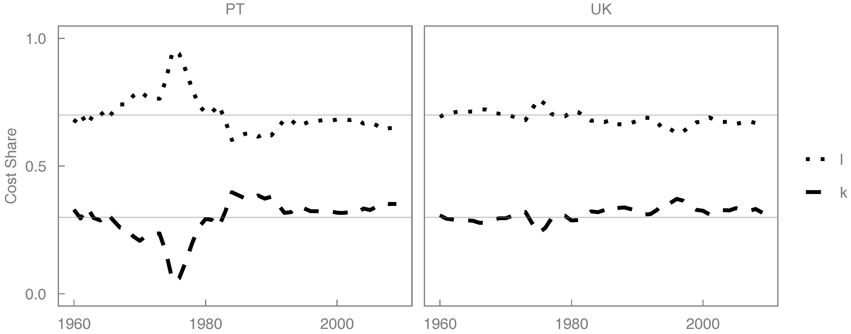
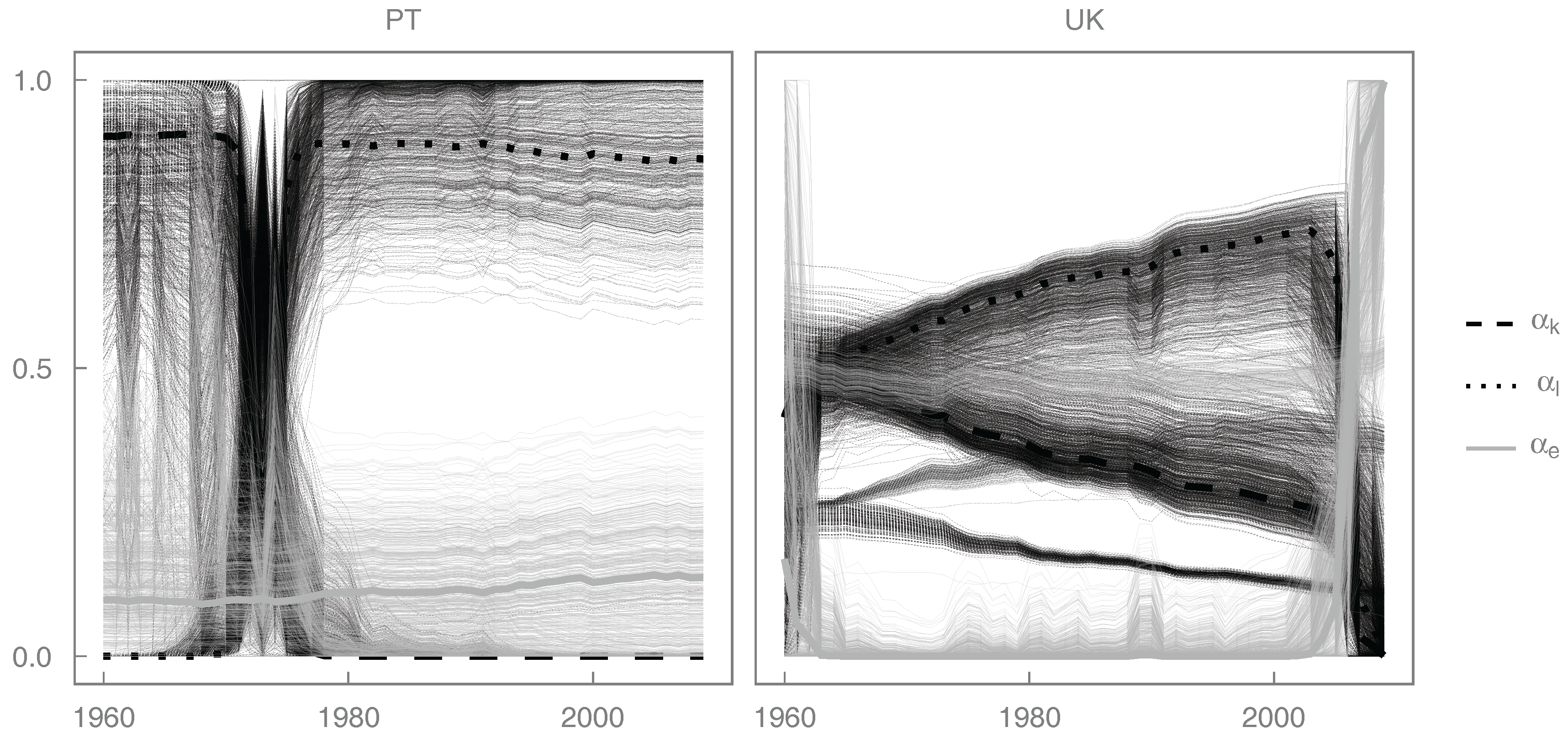
Historically, a stylized fact observed across countries verifies stable long-run cost shares for factors of production, with labor receiving approximately 70% of total income and capital the remaining 30%. This is true for both Portugal and the UK over the time period covered by this study. (See Figure 2.) Typically, payments to energy are less than 10% of GDP [52]. Because direct payments to energy are much smaller than payments to capital or labor, energy is attributed (by the CSP) a correspondingly small output elasticity. These assumptions and observations naturally lead to mainstream modeling approaches in which choices are made to exclude energy as a factor of production, favor the Cobb-Douglas APF (which is homogenous and of degree one), and adhere to the CSP.

However, there may be good reasons to reject the a-priori imposition of each of those choices. And recent literature questions whether the assumptions leading to the CSP are tenable. Two examples are relevant.

First are examples of studies that have adopted alternatives to the assumptions of mainstream economics. Because it is considered to be an intermediate input, the cost of energy is seen as a payment to the owners of primary factors of production for the services provided either directly or embodied in the intermediate factors of production [53]. The use of “Gross-output” APFs [54] allows intermediate factors of production (such as energy) to drive economic growth. Gross output measures of economic output differ from value-added measures of output by including energy as a regular factor of production alongside capital and labor. Although gross output approaches provide a more-complete picture of production processes, and therefore have intuitive appeal, they impose greater demands on data availability. A second alternative to the assumptions of mainstream economics are biophysical growth models [55] that assume energy is the only primary factor of production. (In such models, capital and labor are treated as flows of capital consumption and labor services, computed in terms of the embodied energy use associated with them). From this biophysical point of view, it is argued that energy has a small cost share not because it is relatively less important than either capital or labor as a factor of production; rather energy has a small cost share because it has been abundant and cheap thanks to the free work of the biosphere and geosphere.

Second, according to Kümmel [56,57,58] and others, the CSP is valid only for equilibrium economies comprised solely of profit-maximizing firms in the absence of technological constraints—conditions that are seldom, if ever, present. It might seem absurd that mainstream economics employs the CSP, which is based on assumptions that have never been true, are not now true, and never will be true, but such “ideal” cases are common in many fields. For example, a Carnot heat engine has never, does not, and will never exist, but it is useful as an “ideal” machine against which all real machines are compared. The CSP and models that follow from it play a similar role in economics. (See Acemoglu [59] for a neoclassical derivation of the CSP. See Kümmel et al. [57] for a derivation involving shadow prices and for an excellent discussion of issues surrounding the CSP.)

These examples show that one need not follow the mainstream approach of employing the CSP to obtain constant output elasticities and exclude energy as a factor of production. A different approach to determining output elasticities should be pursued: they cannot be equated to cost shares a-priori. A standard technique, if one rejects the CSP, is to estimate economic growth model parameters (including output elasticities) by fitting models to historical data.

If we want to preserve the choice to reject the CSP, justification for assuming that output elasticities are constant with respect to time (as in the C-D APF) is removed. Indeed, in real economies output elasticities may change as the structure of the economy evolves and as technological constraints on production ebb and flow. Because output elasticities are constant with respect to time in the C-D APF (Equations (1) and (2)), rejecting the CSP leads away from Cobb-Douglas models. A common APF that provides time-varying output elasticities is the CES production function (Equations (3) and (4)), the focus of this study.

When generalizing the two-factor CES production function to include a third factor of production (e.g., energy in Equation (4)), the question arises as to where it feeds into the economic system [60]. There is no a-priori mathematical justification to prefer one nesting structure over another (see Table 1), and the appropriate choice of nesting structure is an unsettled issue in both the theoretical and empirical literature [61]. When adding a third factor of production, the $\left(kl\right)e$ nesting structure is used broadly, probably following the traditional “value-added approach”, whereby capital and labor are incorporated first to form a composite input that is secondarily combined with energy [62]. But the $\left(ek\right)l$ nesting structure has appeared in various models, reflecting an assumption that capital and energy are combined first [63]. And Shen and Whalley [34] argue that the $\left(le\right)k$ nesting structure is appropriate for China.

The choice of the grouped factors of production raises the issue of “separability”, the requirement that the substitution elasticity between paired inputs remains the same, regardless of whether an additional (third) factor of production has been added [64]. Moreover, the cross-elasticities between the nested factors of production and the third factor of production must be equal (e.g., the elasticities between k and e and between l and e in the $\left(kl\right)e$ nesting structure). Typically, separability is merely assumed rather than tested.

Furthermore, in our experience, parameter estimates may differ substantially depending on the nesting structure employed. Unfortunately, few studies methodically assess the effect of nesting structure. (Kemfert [65], Van der Werf [16], and Shen and Whalley [34] provide exceptions.) In the literature, nesting structure is often decided a-priori, either without comment or based on commitments made in Step 1 (Select a theoretical framework).

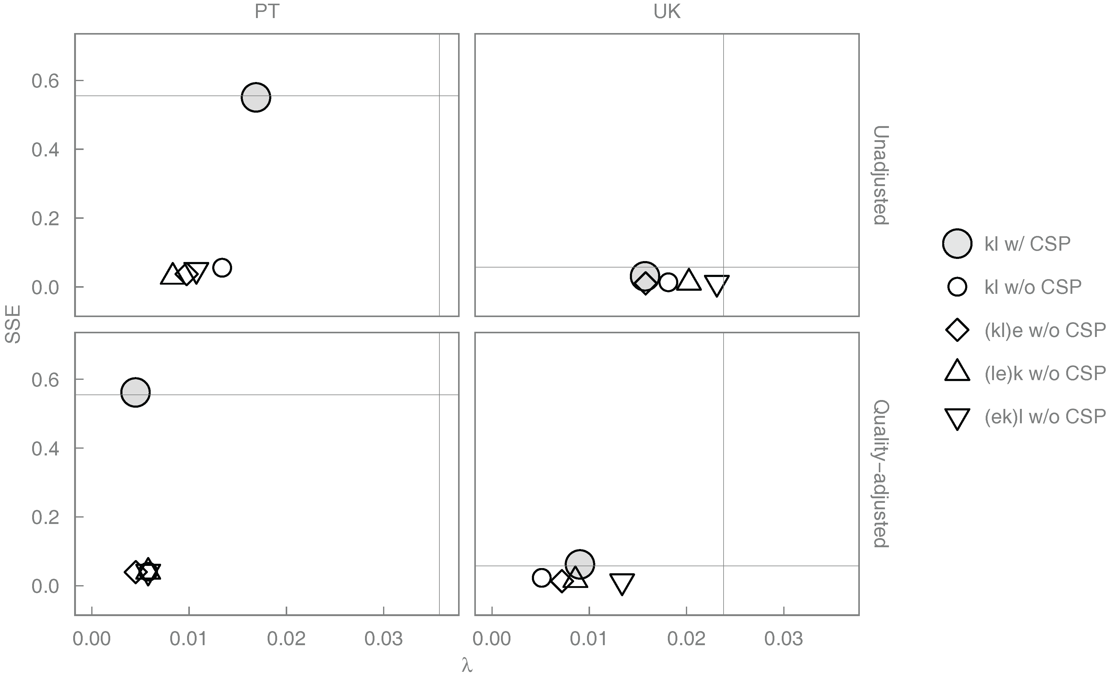
To clarify the above issues and facilitate comparisons among various modeling approaches, we consider three distinct modeling choices: (1) whether (or not) to include energy as a factor of production; (2) whether (or not) to assume the CSP; and (3) which APF to use. We note that CES nesting structure is an aspect of the third modeling choice.

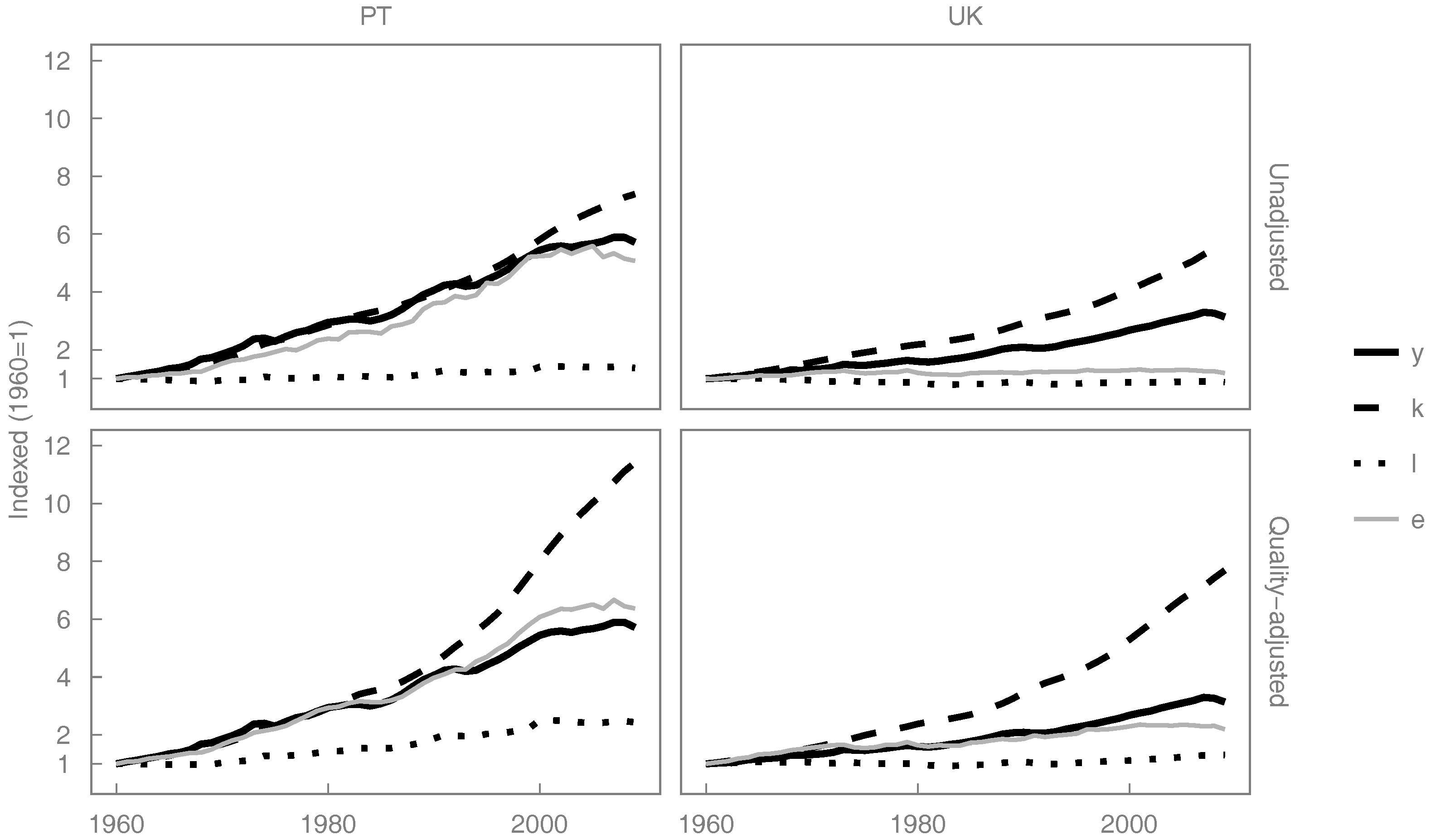
A fourth modeling choice is largely orthogonal to the above considerations and comprises choices relating to the methods used to quantify the factors of production. Most empirical studies of economic growth quantify capital and labor by unadjusted values such as monetary value for capital and work hours for labor [49,66,67]. However, not all capital and labor are equally productive: different capital assets provide different services to economic production, and skilled workers are more productive than unskilled ones. In the relevant literature, there are studies that consider quality-adjusted capital (measuring the productive effect of capital stocks as capital services) and quality-adjusted labor (e.g., adjusting work hours by educational indexes), with the latter [68,69] being more common than the former [70,71]. Indeed, accounting for capital services is a newer field of study, and Inklaar [72] suggests significant measurement issues remain, such as the choice of the rates of return. Work continues in academia [73] and in government [74] to develop consistent datasets of capital services.

Energy, too, has unadjusted and quality-adjusted quantifications. Unadjusted energy is quantified by the thermal equivalent of primary (extracted) energy: the quantity of heat that could be produced from a primary energy carrier. Energy can be quality adjusted on an economic or a physical basis, as discussed by Cleveland et al. [75] and Stern [76], among others. The economic approach commonly involves a price-based Divisia index to allocate greater weight to those energy carriers (such as electricity) that have a higher cost per unit of unadjusted (thermal) energy (in units of $/GJ). In contrast, physical approaches are based on physical attributes of energy only and are founded on the laws of thermodynamics. In our case, we adopt a physical approach with exergy as the quantification for quality-adjusted energy. The second law of thermodynamics quantifies (via the concept of entropy) the observation that work can be completely converted into heat, but the converse is not true. Exergy, based on the second law, is a measure of energy that describes its ability to do physical work. Thermodynamically, exergy is defined as the maximum possible work that could be done by a system as it comes to equilibrium with its surroundings. Quantifying all forms of energy as exergy changes the numerical relationship between work and heat, thereby accounting for energy’s quality. Our approach has two beneficial characteristics: (1) it avoids mixing economic and physical attributes of energy and (2) it obeys the first and second laws of thermodynamics (by virtue of the exergy quantification).

Our approach to quality-adjusting energy is based on the work of Ayres and Warr [51,77,78,79] who argue that the energy factor of production should be quantified as exergy at its point of use in an economy (useful exergy) as opposed to the point of extraction from the biosphere (primary exergy) or at the point when it is sold to final consumers (final exergy), because useful exergy is closer to productive processes and, therefore, more closely correlated to economic activity. From a thermodynamic point of view, measuring energy input to the economy as useful exergy makes sense: it takes physical work at the point of energy dissipation into heat to extract and transform raw materials, fabricate goods and generate services, distribute products, and consume and dispose goods and services in a real economy. Useful exergy can be seen as a quality-adjusted measure of energy, similar to service-adjusted capital and education-adjusted labor. Quality-adjusting (or not) all factors of production (capital, labor, and energy) is our fourth modeling choice.

There are other possible modeling choices in addition to the four discussed above, fitting technique and quantification of economic output among them. However, for this paper, we use a single, rigorous fitting technique in all modeling approaches (see Section 3.3), and we quantify economic output by GDP only. Although the four modeling choices for this paper do not comprise the full set of modeling choices, they provide a sufficiently wide space within which to explore the effect on policy of decisions made throughout the theory-to-policy process.

We thus arrive at our starting point. Fitting APFs to historical data is at the core of an important theory-to-policy process, with the energy-augmented CES production function increasing in popularity. However, few studies critically evaluate, let alone articulate, the theory-to-policy process or examine the impacts of the modeling choices discussed above through to policy. So the time is right for a thorough, detailed, and rigorous evaluation of the theory-to-policy process and the effects of upstream modeling choices on energy and economic policymaking, with particular attention paid to the role of the CES production function.

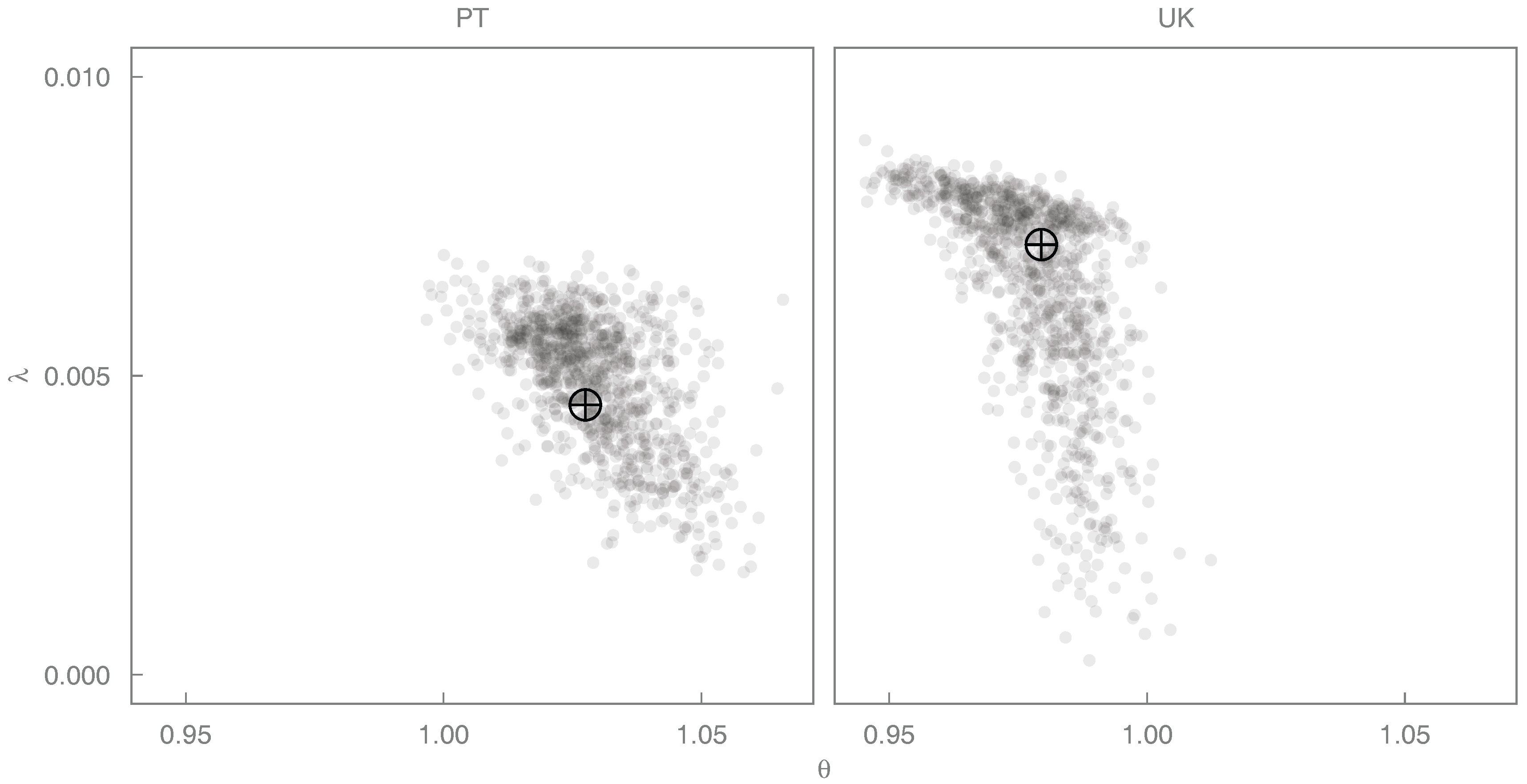
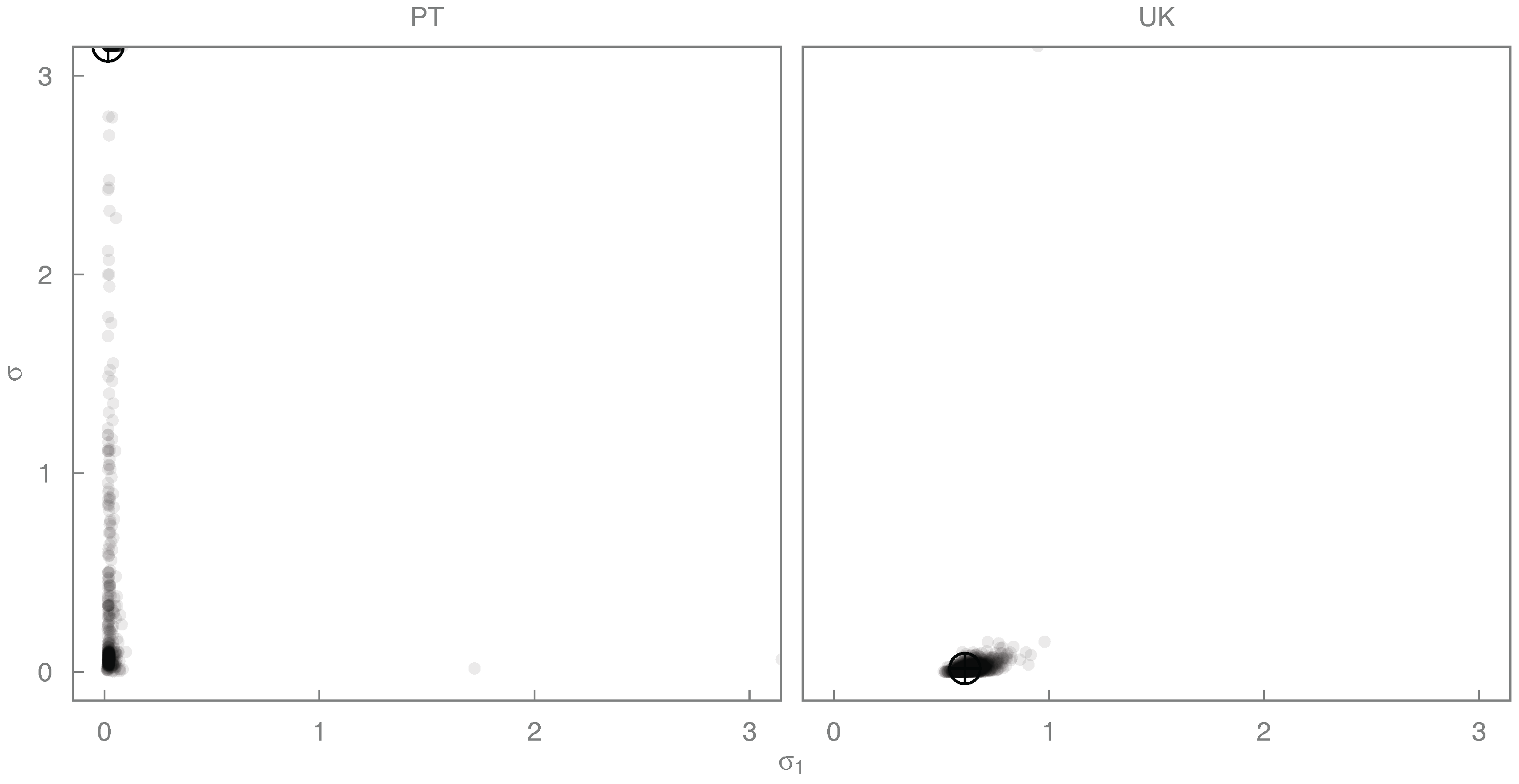
The remainder of this paper performs this evaluation by investigating the effects on policymaking of four modeling choices: (a) including (or not) energy as a factor of production; (b) rejecting (or not) the cost-share principle (CSP); (c) CES nesting structure; and (d) quality-adjusting (or not) the factors of production. We utilize historical data for Portugal and the UK for the time period 1960–2009. Furthermore, we perform bootstrap resampling on one CES production function to give an indication of the precision with which CES parameters can be estimated. We know of no previous studies that perform a similarly comprehensive, quantitative, and rigorous evaluation of the theory-to-policy process and the role of APFs therein.

3. Methods and Historical Data

3.1. Reference Model

In this paper, we work with the Constant Elasticity of Substitution (CES) APF, but we also define an exponential-only reference model:

$$y=\theta {\mathrm{e}}^{\lambda t}.$$

(5)

In the reference model, all economic growth is attributed to λ, thus providing an estimate of the overall economic growth rate for an economy.

3.2. Output Elasticities

Output elasticities (α) appear directly as constant parameters in the C-D APF (Equations (1) and (2)). As discussed in Section 2.3 above, output elasticities for the CES APF (Equation (4)) are not constant; rather, they vary with factors of production over time.

$${\alpha }_{x_1}\equiv \frac{\frac{\partial y}{\partial x_1}}{\frac{y}{x_1}}=\frac{\delta {\delta }_1{x}_1^{-{\rho }_1}{\left[{\delta }_1{x}_1^{-{\rho }_1}+\left(1-{\delta }_1\right)x_2^{-{\rho }_1}\right]}^{\frac{\rho }{{\rho }_1}-1}}{\delta \left[{\delta }_1{x}_1^{-{\rho }_1}+\left(1-{\delta }_1\right)x_2^{-{\rho }_1}\right]{}^{\frac{\rho }{{\rho }_1}}+(1-\delta )x_3^{-\rho }}$$

(6)

$${\alpha }_{x_2}\equiv \frac{\frac{\partial y}{\partial x_2}}{\frac{y}{x_2}}=\frac{\delta \left(1-{\delta }_1\right)x_2^{-{\rho }_1}\left[{\delta }_1{x}_1^{-{\rho }_1}+\left(1-{\delta }_1\right)x_2^{-{\rho }_1}\right]{}^{\frac{\rho }{{\rho }_1}-1}}{\delta \left[{\delta }_1{x}_1^{-{\rho }_1}+\left(1-{\delta }_1\right)x_2^{-{\rho }_1}\right]{}^{\frac{\rho }{{\rho }_1}}+(1-\delta )x_3^{-\rho }}$$

(7)

$${\alpha }_{x_3}\equiv \frac{\frac{\partial y}{\partial x_3}}{\frac{y}{x_3}}=\frac{1-\delta }{\delta x_3^{\rho }\left[{\delta }_1{x}_1^{-{\rho }_1}+\left(1-{\delta }_1\right)x_2^{-{\rho }_1}\right]{}^{\frac{\rho }{{\rho }_1}}+1-\delta }$$

(8)

Using Equations (6)–(8), it can be verified that ${\alpha }_{x_1}+{\alpha }_{x_2}+{\alpha }_{x_3}=1$, thereby demonstrating that Equations (3) and (4) assume constant returns to scale. There are generalizations (not presented here) of the CES APF that allow for non-constant returns to scale. See Appendix B for derivations of Equations (6)–(8).

An interesting question arises when the CES APF is the focus of a study (as it is here): what type of CES model adheres to the CSP? Equations (6)–(8) show that unless the CES model collapses to a C-D model (i.e., ${\rho }_1\to 0$ and $\rho \to 0$), output elasticities will depend on the values of the factors of production (k, l, and e) and, therefore, change over time. And as discussed above, applying the CSP usually means that energy is neglected as a factor of production because of its relatively small cost share. Thus, when we refer to a CES model that adheres to the CSP, we mean a C-D model with (a) capital and labor as the only factors of production (Equation (1)) and (b) ${\alpha }_k$ and ${\alpha }_l$ fixed and equal to their (approximately constant) historical values (Figure 2) rather than fitted to the data being analyzed.

3.3. Parameter Estimation

3.3.1. Technique

Step 2 (Formulate modeling approaches) includes selecting a technique to fit the APFs to historical data. For all modeling approaches analyzed in this paper, we use an ordinary least squares (OLS) approach. The objective of the OLS analysis is minimization of the sum of squared errors (SSE):

$$\mathrm{SSE}=\sum _i{r}_i^2,$$

(9)

where $r_i\equiv ln(y_i/{\widehat{y}}_i)$ is the $i^{\mathrm{th}}$ residual (all models assume multiplicative errors), and ${\widehat{y}}_i$ is the fitted value for economic output at time $t_i$.

Step 3 (Fit to historical data) involves fitting APFs to historical data. For this paper, fitting to historical data provides estimates for values of unknown parameters in CES and reference models ($\widehat{\theta }$, $\widehat{\lambda }$, ${\widehat{\alpha }}_k$, ${\widehat{\alpha }}_l$, ${\widehat{\delta }}_1$, $\widehat{\delta }$, ${\widehat{\rho }}_1$, and $\widehat{\rho }$). We used the R [80] package micEconCES [28] to fit CES models and standard linear model routines to fit other models.

Boundaries of the economically-meaningful region for CES production functions (Equations (3) and (4)) are given by all combinations of ${\delta }_1$ = 0 or 1, δ = 0 or 1, ${\rho }_1$ = $-1$ or ∞, and ρ = $-1$ or ∞.

Table 2. Constant Elasticity of Substitution (CES) boundary models (rows 1–20) and the generic three-factor CES equation (bottom row). Factors of production ($x_1$, $x_2$, $x_3$) are permutations of capital, labor, and energy (k, l, e). Recall that ${\sigma }_1$ (and σ) in the third (and fifth) columns and ${\rho }_1$ (and ρ) in equations are related by ${\sigma }_1=\frac{1}{1+{\rho }_1}$ (and $\sigma =\frac{1}{1+\rho }$). The economically-meaningful ranges of model parameters are $0\le \delta ,{\delta }_1\le 1$ and $0\le \sigma ,{\sigma }_1<\infty$. A blank space indicates a parameter that must be fitted in the boundary model of that row, because it appears in the model. “—” indicates a parameter that cannot be determined by fitting the boundary model of that row, because it does not appear in the boundary model. Note that there are three possible states (lower boundary, unspecified, upper boundary) for four constrained parameters (${\delta }_1$, ${\sigma }_1$, δ, σ), which gives $3^4=81$ possible boundary models. But many boundary parameter combinations yield equivalent CES boundary models. For example, all boundary parameter combinations that include $\delta =0$ yield the same boundary model, $y=\theta A{x}_3$. Thus, there are far fewer unique boundary models (20) than the total number of degenerate boundary equations [81].

	${\mathit{\delta }}_1$	${\mathit{\sigma }}_1$	δ	σ	Boundary Model
1.	1	—	1	—	$y=\theta A{x}_1$
2.	0	—	1	—	$y=\theta A{x}_2$
3.	—	—	0	—	$y=\theta A{x}_3$
4.	—	0	1	—	$y=\theta Amin(x_1,x_2)$
5.	1	—	—	0	$y=\theta Amin(x_1,x_3)$
6.	0	—	—	0	$y=\theta Amin(x_2,x_3)$
7.		∞	1	—	$y=\theta A\left[{\delta }_1{x}_1+(1-{\delta }_1)x_2\right]$
8.	1	—		∞	$y=\theta A\left[\delta x_1+(1-\delta )x_3\right]$
9.	0	—		∞	$y=\theta A\left[\delta x_2+(1-\delta )x_3\right]$
10.			1	—	$y=\theta A{\left[{\delta }_1{x}_1^{-{\rho }_1}+\left(1-{\delta }_1\right)x_2^{-{\rho }_1}\right]}^{-1/{\rho }_1}$
11.	1	—			$y=\theta A{\left[\delta x_1^{-\rho }+\left(1-\delta \right)x_3^{-\rho }\right]}^{-1/\rho }$
12.	0	—			$y=\theta A{\left[\delta x_2^{-\rho }+\left(1-\delta \right)x_3^{-\rho }\right]}^{-1/\rho }$
13.	—	0	—	0	$y=\theta Amin(x_1,x_2,x_3)$
14.	—	0		∞	$y=\theta A\left[\delta min(x_1,x_2)+\left(1-\delta \right)x_3\right]$
15.		∞	—	0	$y=\theta Amin\left[{\delta }_1{x}_1+\left(1-{\delta }_1\right)x_2,x_3\right]$
16.		∞		∞	$y=\theta A\left\{\delta \left[{\delta }_1{x}_1+\left(1-{\delta }_1\right)x_2\right]+\left(1-\delta \right)x_3\right\}$
17.	—	0			$y=\theta A{\left\{\delta {\left[min\left(x_1,x_2\right)\right]}^{-\rho }+\left(1-\delta \right)x_3^{-\rho }\right\}}^{-1/\rho }$
18.			—	0	$y=\theta Amin\left\{{\left[{\delta }_1{x}_1^{-{\rho }_1}+\left(1-{\delta }_1\right)x_2^{-{\rho }_1}\right]}^{-1/{\rho }_1},x_3\right\}$
19.				∞	$y=\theta A\left\{\delta {\left[{\delta }_1{x}_1^{-{\rho }_1}+\left(1-{\delta }_1\right)x_2^{-{\rho }_1}\right]}^{-1/{\rho }_1}+\left(1-\delta \right)x_3\right\}$
20.		∞			$y=\theta A{\left\{\delta {\left[{\delta }_1{x}_1+\left(1-{\delta }_1\right)x_2\right]}^{-\rho }+\left(1-\delta \right)x_3^{-\rho }\right\}}^{-1/\rho }$
					$y=\theta A{\left\{\delta {\left[{\delta }_1{x}_1^{-{\rho }_1}+\left(1-{\delta }_1\right)x_2^{-{\rho }_1}\right]}^{\rho /{\rho }_1}+\left(1-\delta \right)x_3^{-\rho }\right\}}^{-1/\rho }$

shows the set of 20 degenerate boundary equations found along parameter boundaries. Each degenerate equation provides a boundary model.

Fitting along boundaries is important for two reasons. First, bounded, non-linear, ordinary least squares (OLS) algorithms that perform gradient searches within the parameter space (such as the PORT and L-BFGS-B algorithms that we employ in R) often have difficulties dealing with boundaries. Fitting directly on the boundaries of the economically-meaningful region ensures that a sum of squared errors (SSE) minimum located on a boundary will be found, if it exists. Second, fitting on the boundaries of the economically-meaningful region prevents erroneous reporting of unknowable parameters.

Table 2 indicates parameters that are unknowable in the boundary models. For example, ${\sigma }_1$ and σ are unknowable in the boundary model shown in Row 1 of Table 2. If an OLS search algorithm (such as PORT and L-BFGS-B, discussed above) operating with the full CES model (bottom row of Table 2) were to find an SSE minimum along that boundary, it would report ${\widehat{\sigma }}_1$ and $\widehat{\sigma }$ in addition to $\widehat{\theta }$, $\widehat{\lambda }$, ${\widehat{\delta }}_1$ (which will be unity), and $\widehat{\delta }$ (also unity). Under these conditions, it is clearly erroneous to report meaningless values for ${\widehat{\sigma }}_1$ and $\widehat{\sigma }$. Fitting with the boundary models shown in Table 2 avoids this mistake.

Boundary models obtained when ${\delta }_1$ or δ is at an extreme value (0 or 1) are straightforward to derive from the bottom row of Table 2. When ${\sigma }_1$ or σ is 0, factors of production are perfect complements and the Leontief model applies (e.g., when ${\sigma }_1=0$ and $\delta =1$, the Leontief model is $y=\theta Amin(x_1,x_2)$, row 4 in Table 2). When ${\sigma }_1$ or σ is ∞, factors of production are perfect substitutes and the linear model applies (e.g., when ${\sigma }_1=\infty$ and $\delta =1$, the linear model is $y=\theta A\left[{\delta }_1{x}_1+(1-{\delta }_1)x_2\right]$, row 7 in Table 2). If the fitted parameters in a boundary model violate constraints, the boundary model is rejected.

We used customized code to fit all boundary models (i.e., every equation in Table 2) and to select from all models (those in the interior of the parameter space and those on the boundaries) the one with smallest SSE that also satisfies the contraints of the parameter space. In special cases, two boundary models will be equivalent. For example, boundary model 4 is identical to boundary model 1 (2) if $x_1$ is always less than (greater than) $x_2$ for all years. If two or more models have the same SSE (to ten digits), the model with the lowest row number in Table 2 is deemed the winning model.

Section 4 provides graphs of estimated parameters and $\widehat{\alpha }$ time series. Appendix C gives tables of all estimated parameters.

3.3.2. Precision

Determining the precision of estimated parameters in Step 3 (Fit to historical data) is important but challenging. It is quite possible for substantial changes in a parameter to have a relatively modest effect on the objective function that is determining the parameter estimates (in our case, SSE). When this happens, the best estimate is not much better than many other estimates, and parameter estimates should be interpreted with caution. For this paper, we use bootstrap resampling as a way to estimate parameter precision. (See Efron [81] and Diciccio and Efron [82] for the general approach and Section 4.2.3 for additional comments.)

Bootstrapping is a statistical technique for estimating the precision of parameter estimates by exploring the distribution of estimates in many resampled data sets. Each resampled data set is a randomized version of the original sample data to which the desired analysis method can be applied. Resampled data sets can be formed in a number of ways in accordance with the type of data, experimental design, and modeling assumptions involved. By investigating the variability of a parameter estimate from one resampled data set to another, one can learn about the precision of the estimation method.

In the context of linear models (regression), resamples are generally created by residual resampling. In our case, we formed resamples by adding to the fitted response ($ln(\widehat{y}$)) the product of a residual from the original model fit and random sign ($-1$ or 1, each with probability $0.5$). Intuitively, this method assumes that the residuals are indicative of the variability (from many potential sources) inherent in the data such that it would be unsurprising if the residual from any particular year had been observed in a different year. Thus, a resampled response $ln\left({\tilde{y}}^{\prime }\right)$ can be computed as

$$ln\left({\tilde{y}}_i^{\prime }\right)=ln\left({\widehat{y}}_i\right)\pm r_j,$$

(10)

where $r_i\equiv ln(y_i/{\widehat{y}}_i)$. Both the sign (±) and the index of the residual (j, typically different from i) are chosen at random (with replacement). We repeated the resampling process 1000 times for each combination of growth model and country.

The coefficients from the fit to a resampled time series (the “resample coefficients”) will be different from the coefficients obtained from the fit to historical data (the “base coefficients”) and form a “resample distribution”. When these resample coefficients are highly variable, it is an indication that the data do not determine the parameter estimates very precisely. Even when the residuals are small and the model produces fitted values that track the observed data closely, it may still be difficult to estimate some or all of the model parameters precisely. Lack of precision can stem from a number of factors, including a poor model fit, low model sensitivity to one or more parameters, correlation among parameter estimates, variability unexplained by the predictors in the model, etc.

We choose the resampling approach instead of the more-common technique of estimating symmetric confidence intervals from standard errors for two reasons. First, the economically-meaningful region is highly constrained (as discussed in Section 3.3.1), and symmetric confidence intervals often violate the constraints. For example, an estimate of ${\widehat{\delta }}_1=0.25\pm 0.3$ is nonsensical, because ${\delta }_1\in [0,1]$. Second, true confidence intervals for constrained parameters are often asymmetric (e.g., ${\delta }_1=0.3+0.1,-0.05$), but the standard error approach yields symmetric confidence intervals. Our resampling approach both respects constraints and allows for asymmetric descriptions of parameter precision.

Section 4 provides resampling distributions for all estimated parameters for modeling approaches that reject the CSP, include energy, use quality-adjusted factors of production, and employ the $\left(kl\right)e$ nesting structure.

3.4. Data

Step 2 (Formulate modeling approaches) includes selecting historical data to quantify factors of production and economic output. Following Klump and Preissler [83], we normalize all historical data (y, k, l, and e), meaning aggregate values are indexed by ratio relative to an initial year ($t_0$), while time (t) is indexed by difference relative to the initial year. After normalizing, $\widehat{\theta }$ is expected to be near 1.

Our empirical analysis focuses on Portugal and the United Kingdom for the 50-year period 1960–2009, thereby avoiding economic shocks associated with the World Wars and allowing for the use of international statistics that generally go back only as far as 1960. Figure 3 shows indexed historical data, and

Table 3. Measures and sources of economic output and factors of production.

Variable	Measure/Units	Source of Data
		Portugal	United Kingdom
Economic output
Output (Y)	Gross domestic product in US$	PWT8.1 [84]	PWT8.1 [84]
Unadjusted factors of production
Capital (K)	Stocks in volume index	da Silva and Lains [85]	Oulton and Wallis [86]
Labor (L)	Total hours worked	PWT8.1 [84]	PWT8.1 [84]
Energy (E)	Primary exergy in joules	Palma et al. [87]	Brockway et al. [88]
Quality-adjusted factors of production
Capital (K)	Services in volume index	da Silva and Lains [85]	Oulton and Wallis [86]
Labor (L)	Total hours worked	PWT8.1 [84]; Barro and Lee [73]	PWT8.1 [84]; Barro and Lee [73]
Energy (E)	Useful exergy in joules	Palma et al. [87]	Brockway et al. [88]

summarizes the sources for these data.

3.4.1. Output (y)

There are several options for quantifying economic output, including Gross Output, Gross Value Added, and GDP (most common for studies of this type). We follow convention, quantifying economic output as GDP at constant prices in 2005 USD from the Penn World Tables [84].

3.4.2. Factors of Production (k, l, and e)

Any measure of capital, labor, or energy that fails to account for qualitative differences among these factors of production may result in a less precise quantification of their effective contribution to output. Details of the approach to obtain each of these measures are summarized below and discussed in detail in Appendix A.

Capital (k)

The standard (unadjusted) approach to quantifying capital is to account for aggregate asset stocks using the perpetual inventory method. However, these stock measures do not account for the heterogeneous contribution to production from assets of varying type and vintage. By measuring the flow of productive services from the cumulative stock of past investments, capital services accounts more accurately for the contribution of capital to production.

We adopt net capital stock and volume index of capital services as aggregate measures for unadjusted and quality-adjusted capital, respectively. For Portugal, data are obtained from da Silva and Lains [85]; for the UK, data are obtained from Oulton and Wallis [86]. Note that although both country-specific studies used in our analysis adopt the same basic approach to obtain stocks and services measures for capital (pioneered by the US Bureau of Labor Statistics), they differ in several assumptions (e.g., number of asset categories and tax adjustments) and are therefore not directly comparable. However, each constitutes the best and most complete accounting of integrated capital stocks and services available for that country. (“Integrated” in the sense that both capital stocks and services are estimated by a methodology that uses the same data to produce both capital stocks and, following, capital services.) For details see Appendix A.1.

Labor (l)

The standard (unadjusted) method to quantify labor accounts for either total number of workers or hours worked by engaged individuals. Both measures assume all workers are equally productive. In fact, the productive contribution from one hour of work depends on the worker’s skills, which can be proxied by measurable human capital characteristics, such as the average years of schooling.

We adopt aggregate hours worked by engaged individuals [84] as a measure for unadjusted labor. Quality-adjusted labor is estimated by multiplying unadjusted labor by a human capital index, computed from educational attainment data [73].

Energy (e)

Energy inputs are generally aggregated by summing the thermal equivalent of each energy carrier (in BTUs or joules). However, this approach ignores qualitative differences between energy types. Accounting for energy inputs using an exergy metric and measuring energy flows at their useful stage—after all transformation and conversion losses and just before becoming energy services in the economy—allows weighting of energy inputs according to their capacity to deliver economically productive work at the point of use [77].

We adopt aggregate primary exergy supply and useful exergy consumption as measures for unadjusted and quality-adjusted energy, respectively. Data are obtained from two of the recently-emerging, country-specific useful exergy accounting studies: for Portugal, Palma et al. [87]; for the UK, Brockway et al. [88].

3.4.3. Cost Shares of Capital and Labor

Historical annual cost shares associated with capital and labor are computed from data available at the European Commission’s Annual Macro-Economic Database [89]. (See Figure 2.) Aside from one shock in the 1970s and in conformity with the Kaldor facts [90], these cost shares are nearly constant, 30% of payments to capital and 70% of payments to labor, the proportions typically observed for industrialized countries [59]. Some fluctuations can be observed for both countries, such as the 1973 oil crisis, which led to a decrease in the payments to capital. For Portugal, the effect of the oil crisis is combined with the much more significant impact on the payments to labor and capital brought about by the Carnation Revolution of 1974. Despite these significant shocks, cost shares return to their long-term values.

4. Results

This section reports results from fitting APFs to historical data using various modeling approaches. Interpretation of the results through to policy is deferred to Section 5.

4.1. Fits to Historical GDP

In Figure 4, fitted economic output ($\widehat{y}$) is compared with historical economic output (y) for each modeling approach. Most modeling approaches fit historical data very well. It is noteworthy that the reference model (Equation (5)) provides a good fit to historical data for the UK, leaving little opportunity for improvement by adding factors of production or by choosing among different nesting structures.

Residual plots for each modeling approach are shown in Appendix C.2. Visual inspection of Figure A1 indicates that none of the modeling approaches display heterscedasticity, but the reference model and the modeling approach that adheres to the CSP are poorly specified. Because we assess parameter precision via bootstrap resampling (Section 3.3.2) which is not predicated on a normality assumption, inspection of resampling distributions (Figures 7–10) is a more useful diagnostic than tests for normality based on residuals.

4.2. Parameter Estimates

The following subsections present, in graphical form, parameter estimates resulting from the parameter estimation process described in Section 3.3. See Appendix C.1 for tables of estimated parameters.

4.2.1. Solow Residuals ($\widehat{\lambda }$) and Sum of Squared Errors (SSE)

Figure 5 shows Solow residuals ($\widehat{\lambda }$) and sum of squared errors (SSE) for all models. Vertical and horizontal grid lines show λ and SSE, respectively, for the reference model (Equation (5)).

We note that in the reference model, all economic growth is attributed to the Solow residual (λ). When all of y, k, l, and e are ≥1, the reference model will have a larger estimated Solow residual ($\widehat{\lambda }$) than any CES model, because no factors of production are included in the reference model to drive economic growth, but the non-A part of a CES model will be ≥1, typically driving $\widehat{\lambda }$ to be smaller (assuming, as is typical, that $\widehat{\theta }$ is close to 1).

On the other hand, it is not necessarily true that CES models (Equations (3) and (4)) will exhibit lower SSE than the reference model (Equation (5)). The CES APFs have more parameters, but there is no set of parameters values (θ, λ, ${\delta }_1$, δ, ${\rho }_1$, and ρ) that eliminates the factors of production (k, l, and e) from the CES models, thereby reproducing the reference model. If the factors of production are poorly correlated to economic output (y), SSE may be higher for a CES model than for the reference model, as seen for quality-adjusted factors of production with the CSP and the $kl$ nesting ( ) for both Portugal and the UK.

4.2.2. Output Elasticities for Capital (${\alpha }_k$), Labor (${\alpha }_l$), and Energy (${\alpha }_e$)

The estimated output elasticities (${\alpha }_i$) resulting from the parameter estimation procedures in Section 3.3 are presented in Figure 6 for all modeling approaches.

There should be no expectation that output elasticities estimated from CES APFs that reject the CSP (shown in the “w/o CSP” rows of Figure 6) would look anything like output elasticities estimated from either (a) any modeling approach that assumes the CSP (the “w/ CSP” row in Figure 6) or (b) any modeling approach in which output elasticities are determined by fitting a C-D APF to historical data. Equations (6)–(8) show that output elasticities derived from the CES APF are functions of the factors of production, which change over time. When the CSP is assumed to be valid (as in the “w/ CSP” rows of Figure 6), output elasticities are equated to cost shares which are approximately constant through time (see Figure 2), leading to output elasticities that are approximately constant through time. When output elasticities are determined by fitting a C-D APF to historical data, the output elasticities may be different from historical cost shares, but they will still be constant with respect to time.

Our interpretation of the results in Figure 6 is that time-varying output elasticities indicate the time-varying nature of constraints on production. When output elasticity for a factor of production is low, that factor of production is not a notable constraint on economic output. When output elasticity for a factor of production is high, that factor of production is an important constraint on economic output.

That said, the temporal variation of output elasticities in Figure 6 is, for many modeling approaches, extreme; some output elasticities change from 0 to 1 in the span of a few years. Although exogenous circumstances and events can modify the constraints on an economy over time, this behavior is unexpected if one assumes that output elasticities should change gradually from year to year. We note that large ${\widehat{\rho }}_1$ and $\widehat{\rho }$ can make output elasticities unstable, because large exponents in Equations (6)–(8) amplify small changes in factors of production through time. With reference to

Table A3. Elasticities of substitution (${\rho }_1$ and ρ) for all modeling approaches.

Country	Model	CSP	Factors of Prod.	Energy	Nesting Str.	${\mathit{\rho }}_1$	ρ
PT	CES	Adhere	Unadjusted	Without	$kl$	0.000
PT	CES	Reject	Unadjusted	Without	$kl$	5.029
PT	CES	Reject	Unadjusted	With	$\left(kl\right)e$	11.737	−0.428
PT	CES	Reject	Unadjusted	With	$\left(le\right)k$	1.507	72.286
PT	CES	Reject	Unadjusted	With	$\left(ek\right)l$	191.549	4.368
PT	CES	Adhere	Quality-adjusted	Without	$kl$	0.000
PT	CES	Reject	Quality-adjusted	Without	$kl$	57.777
PT	CES	Reject	Quality-adjusted	With	$\left(kl\right)e$	54.582	−1.000
PT	CES	Reject	Quality-adjusted	With	$\left(le\right)k$	55.834	185.640
PT	CES	Reject	Quality-adjusted	With	$\left(ek\right)l$	57.777
UK	CES	Adhere	Unadjusted	Without	$kl$	0.000
UK	CES	Reject	Unadjusted	Without	$kl$	0.941
UK	CES	Reject	Unadjusted	With	$\left(kl\right)e$	0.551	163.988
UK	CES	Reject	Unadjusted	With	$\left(le\right)k$	0.621	1.000
UK	CES	Reject	Unadjusted	With	$\left(ek\right)l$	11.505	−0.074
UK	CES	Adhere	Quality-adjusted	Without	$kl$	0.000
UK	CES	Reject	Quality-adjusted	Without	$kl$	0.720
UK	CES	Reject	Quality-adjusted	With	$\left(kl\right)e$	0.640	58.560
UK	CES	Reject	Quality-adjusted	With	$\left(le\right)k$	−1.000	0.746
UK	CES	Reject	Quality-adjusted	With	$\left(ek\right)l$	7.403	−0.284

, we see that the $kl$ and $\left(le\right)k$ nesting structures for the UK are the only modeling approaches with both ${\widehat{\rho }}_1$ and $\widehat{\rho }$ small (less than 3). Those modeling approaches are also the only modeling approaches that have all of the following characteristics: (a) rejects the CSP, (b) exhibits non-extreme output elasticities that are comparatively stable through time, and (c) exhibits output elasticities that approximate historical cost shares. (See Section 5.4 for additional discussion).

4.2.3. Parameter Precision

As discussed in Section 3.3.2, estimation of parameter precision is important but challenging via the usual statistical techniques. The usual methods for quantifying the precision of parameter estimates using standard errors, confidence intervals, and p-values rely on an asymptotic theory that applies on the interior of a parameter space and assumes independence of error terms. It can be difficult to provide an a priori justification for the use of asymptotic results or to correctly adjust for sample size or potential violations of the model assumptions. The authors of the R package micEconCES acknowledge as much when they say that “As [the computation of the variance-covariance matrix] is only valid asymptotically, we calculate the estimated variance of the residuals … without correcting for degrees of freedom” [28].

Issues may arise when estimated parameters lie on or near a boundary of (the economically meaningful portion of) the parameter space or when the hypothesis of interest lies on the boundary. For example, in an investigation of whether energy is important for economic growth with the ($kl$)e nesting, we may consider the null hypothesis that $\delta =1$ in Equation (4) (energy is not a meaningful factor of production). While there is an asymptotic theory for dealing with such cases (see, e.g., Molenberghs and Verbeke [91]), the distributions are, in general, more complicated and may be difficult to evaluate.

The situation is further complicated in the case of cross-model parameter comparisons, although within-model precision estimates bring us a good deal of the way to answering such questions as whether the data support a claim that, for example, the Solow residual (λ) is larger in the exponential model than in a CES model.

To give an indication of parameter precision, we present results from a bootstrap resampling analysis of CES functions that reject the CSP, include energy, use quality-adjusted factors of production, and employ the ($kl$)e nesting for both Portugal and the UK. To our knowledge, this is the first application of bootstrap resampling techniques to the CES APF.

Figure 7 shows bootstrap resampling distributions for $\widehat{\lambda }$ and $\widehat{\theta }$. Figure 8 shows bootstrap resampling distributions for $\widehat{\delta }$ and ${\widehat{\delta }}_1$. Figure 9 shows bootstrap resampling distributions for time-varying ${\widehat{\alpha }}_k$, ${\widehat{\alpha }}_l$, and ${\widehat{\alpha }}_e$ (Equations (6)–(8) with $\left(kl\right)e$ nesting structure). Figure 10 shows bootstrap resampling distributions for $\widehat{\sigma }$ and ${\widehat{\sigma }}_1$.

Our interpretation of the results in Figure 7, Figure 8, Figure 9 and Figure 10 is that the extent of the bootstrap resampling distribution is an indication of the precision with which parameters are estimated. When larger spread is observed in the resampling distribution, parameters are estimated with less precision. When smaller spread is observed, parameters are estimated with more precision. (See Section 5.3 for applications of this interpretation).

5. Discussion: Cautionary Tales

The results presented in Section 4 highlight several issues that must be addressed with caution when operating in Steps 3–6 of the theory-to-policy process (Fit to historical data, Compare and evaluate modeling approaches, Interpret the economy, and Formulate policy).

5.1. Issues around Step 3 (Fit to Historical Data)

Boundary Models

As discussed in Section 3.3.1, fitting along boundaries is important for two reasons. First, bounded, non-linear, ordinary least squares (OLS) fitting techniques often have difficulties dealing with boundaries. Second, some CES parameters are unknowable on boundaries, and it would be a mistake to report values for such parameters.

In this study, we found one modeling approach that resulted in a boundary model: Portugal with the $\left(ek\right)l$ nesting structure and quality-adjusted factors of production that rejects the CSP. The minimum SSE is found on the boundary that eliminates energy (and nearly eliminates capital), specifically ${\widehat{\delta }}_1=0$ and $\widehat{\delta }\approx 1$. (See

Table A2. Distribution parameters (${\delta }_1$ and δ) for all modeling approaches.

Country	Model	CSP	Factors of Prod.	Energy	Nesting Str.	${\mathit{\delta }}_1$	δ
PT	CES	Adhere	Unadjusted	Without	$kl$	0.300	1.000
PT	CES	Reject	Unadjusted	Without	$kl$	0.984	1.000
PT	CES	Reject	Unadjusted	With	$\left(kl\right)e$	1.000	0.728
PT	CES	Reject	Unadjusted	With	$\left(le\right)k$	0.250	0.000
PT	CES	Reject	Unadjusted	With	$\left(ek\right)l$	0.000	0.983
PT	CES	Adhere	Quality-adjusted	Without	$kl$	0.300	1.000
PT	CES	Reject	Quality-adjusted	Without	$kl$	1.000	1.000
PT	CES	Reject	Quality-adjusted	With	$\left(kl\right)e$	1.000	0.903
PT	CES	Reject	Quality-adjusted	With	$\left(le\right)k$	0.000	0.000
PT	CES	Reject	Quality-adjusted	With	$\left(ek\right)l$	0.000	1.000
UK	CES	Adhere	Unadjusted	Without	$kl$	0.300	1.000
UK	CES	Reject	Unadjusted	Without	$kl$	0.420	1.000
UK	CES	Reject	Unadjusted	With	$\left(kl\right)e$	0.422	1.000
UK	CES	Reject	Unadjusted	With	$\left(le\right)k$	0.758	0.720
UK	CES	Reject	Unadjusted	With	$\left(ek\right)l$	0.008	0.257
UK	CES	Adhere	Quality-adjusted	Without	$kl$	0.300	1.000
UK	CES	Reject	Quality-adjusted	Without	$kl$	0.566	1.000
UK	CES	Reject	Quality-adjusted	With	$\left(kl\right)e$	0.501	0.831
UK	CES	Reject	Quality-adjusted	With	$\left(le\right)k$	0.809	0.621
UK	CES	Reject	Quality-adjusted	With	$\left(ek\right)l$	0.074	0.298

).

In many other modeling approaches, parameter estimates are close to, but not exactly on, a boundary. One example is the modeling approach for Portugal wherein all factors of production are quality-adjusted, the $\left(kl\right)e$ nesting structure is employed, and the CSP is rejected. The best fitting value of ${\delta }_1$ rounds to 1.000. (See Table A2.) However, the value of ${\widehat{\delta }}_1$ is actually slightly less than 1, namely $1-{\widehat{\delta }}_1=3.11\times {10}^{-15}$. (The value of ${\delta }_1$ is 0.99999999999999689, but clearer communication is afforded by reporting $1-{\delta }_1$, the distance between the estimate of ${\delta }_1$ and the boundary of the economically-meaningful region at 1. Note that machine precision is $2.22\times {10}^{-16}$, so the distance between ${\delta }_1$ and the boundary is more than an order of magnitude greater than the precision of 64-bit floating point operations.) The fitting algorithm does, in fact, find a set of parameters that minimizes SSE: the near-boundary model has $\mathrm{SSE}=0.040$, while the model on the boundary where ${\delta }_1=1$ has $\mathrm{SSE}=0.105$. The implications of near-boundary parameter estimates are explored further in Section 5.3.1.

Cautionary tale: Analysts should treat parameter estimates that are close to boundaries of the economically-meaningful space with much care.

5.2. Issues around Step 4 (Compare and Evaluate Modeling Approaches)

5.2.1. Multiple Criteria

There is no single, agreed-upon criterion for selecting preferred modeling approaches from among the modeling approaches developed in Step 2 (Formulate modeling approaches) and fitted in Step 3 (Fit to historical data). Some authors compare a statistical metric that assesses all modeling approaches, which may or may not be different from the objective function of the fitting technique. Examples include SSE or mean squared error [33,39,57,65] and $R^2$ [16,77]. Additional statistical inference procedures can be used to determine whether significant differences exist between rejected and preferred modeling approaches. (See Ayres and Warr [77], Appendix B.) Other authors assess modeling approaches based on estimates for model parameters, such as the Solow residual [13,77], or their standard errors, as in [34] where the model with the smallest standard error for the elasticity of substitution is preferred. Some authors neglect to state criteria used to compare and assess modeling approaches.

In addition, the theoretical framework from Step 1 (Select a theoretical framework) may be be invoked to remove from consideration modeling approaches that contradict its commitments. For example, Jorgenson and Griliches [13] hypothesize that “if real product and real factor input are accurately accounted for, the observed growth in total factor productivity [will be] negligible”. Jorgenson and Griliches’s theoretical framework commits them (a) to decide a best modeling approach based on total factor productivity (A), and (b) consequently to discard modeling approaches that fail to make A negligible.

Cautionary tale: Lacking a standard approach for comparing and evaluating modeling approaches, Step 4 (Compare and evaluate modeling approaches) can be a jumble, allowing each analyst to justify their selection of preferred modeling approaches on whatever grounds believed appropriate.

5.2.2. Multiple Models and the Risk of Overfitting

The consideration of multiple modeling approaches is complicated not only by the fact that there is no single method of selecting preferred modeling approaches, but also by the risk of over-fitting that arises whenever multiple models are considered, regardless of the selection method employed. In fact, many of the selection criteria discussed above tend to favor complicated models, because modeling approaches with additional parameters always fit better than modeling approaches without the additional parameters, assuming the same historical data. This can lead to over-fitting, especially if multiple complex models are considered and compared, and raises the risk of artificially preferring modeling approaches with more-complex APFs. When comparing multiple models with different degrees of freedom, an information criterion (such as AIC) may be helpful.

Often, after considering (or potentially considering) multiple modeling approaches, including some with the same number of degrees of freedom, researchers select a “best” one and the resulting modeling approach is analyzed and interpreted as if it were the only one considered. When the “researcher degrees of freedom” [92] are undisclosed or unaccounted for, the strength of the evidence provided in the data is necessarily inflated. This can lead to an over-interpretation of the results unless corrections are made in a way that is similar to corrections for the “multiple comparisons” problem. This is not the place to elaborate on or advocate for particular solutions to multi-model inference, only to point out that ignoring the issue is not without consequences—consequences that may have an impact in Step 5, (Interpret the economy) and in Step 6 (Formulate policy). (Some of the challenges of multi-model inference and one approach to handling them are provided in Burnham and Anderson [93].)

When multiple modeling approaches lead to similar conclusions, confidence in the results is warranted. On the other hand, when several modeling approaches receive similar scores for the selection metric, data-driven model selection may become unstable: small and relatively uninformative changes to the data (e.g., including an additional year when it becomes available or using a different currency base) may change which modeling approaches are preferred. Similarly, the selection of different modeling approaches for different countries or eras might have little to do with substantive differences in the economy when several modeling approaches are nearly equally good. This is particularly problematic when the competing modeling approaches yield parameter estimates that are not directly comparable.

Cautionary tale: While it is important to consider multiple modeling approaches, doing so complicates analysis as data-driven model selection may be unstable or provide a falsely inflated sense of the strength of the evidence presented in the data. Care must be taken to interpret the selected models in the context of the selection process that was employed.

5.3. Issues around Step 5 (Interpret the Economy)

5.3.1. Parameter Precision

The precision with which parameters are estimated is cause for caution when interpreting economies. As discussed in Section 3.3.2, we use bootstrap resampling as a way to estimate the precision of parameter estimates for modeling approaches that employ the $\left(kl\right)e$ nesting structure, reject the CSP, and use quality-adjusted factors of production. This resampling technique can yield important insights into the way economies should be interpreted. Our results show that both over-interpretation (claiming too much about the economy given the results) and under-interpretation (claiming too little about the economy given the results) are possible.

For example, Table A3 shows $\widehat{\rho }=-1$ ($\widehat{\sigma }=\infty$) for Portugal, indicating substitutability between the capital-labor composite ($kl$) and energy (e). However, Figure 10 shows so little precision for $\widehat{\sigma }$ that claiming substitutability between $\left(kl\right)$ and e would be an over-interpretation of the results. Indeed, it would be unwise to develop economic policy for Portugal in Step 6 (Formulate policy) that is predicated on substitutability between the capital-labor composite and energy in Portugal. Although precision is better for the UK, the sensitivity of interpretation to $\widehat{\sigma }$ means that caution should be exercised for the UK as well.

It is also possible to under-interpret the significance of results. In Section 5.1, we noted that the value of $1-{\widehat{\delta }}_1$ for Portugal is estimated to be $3.11\times {10}^{-15}$ under the modeling approach that employs the $\left(kl\right)e$ nesting structure, rejects the CSP, and uses quality-adjusted factors of production. The fact that the value of ${\widehat{\delta }}_1$ is close to, but not exactly on, the economically-meaningful boundary (${\delta }_1=1$) has significant implications. In Figure 6, we see that the corresponding labor output elasticity (${\widehat{\alpha }}_l$) increases from 0 to 0.9 around the time of the Portuguese Carnation Revolution (1974). This transition would not occur if ${\widehat{\delta }}_1$ were exactly 1 (i.e., on the boundary of the economically meaningful region), as the labor term would be eliminated from Equation (7) (with $\left(kl\right)e$ nesting structure).

The resampling analysis sheds further light on this issue. In this case, none of the 1000 resample models are along the boundary where ${\delta }_1$ is exactly 1. (The minimum value of $1-{\widehat{\delta }}_1$ (maximum value of ${\widehat{\delta }}_1$) in the resampling distribution is $1.22\times {10}^{-15}$, and the middle 95% of the resampling distribution is captured by $6.07\times {10}^{-4}\le 1-{\widehat{\delta }}_1\le 2.55\times {10}^{-15}$. Note that all values of $1-{\widehat{\delta }}_1$ are different from 0 by an amount greater than the machine precision, $2.22\times {10}^{-16}$.) Indeed, Figure 9 shows that all but 13 of the 1000 resample models exhibit the transition to labor dominance. (It is interesting to note that there are 13 outlier models on the boundary ${\widehat{\delta }}_1=0$. For these models, capital is eliminated from the CES APF, and labor dominates from the first year to the last. This can be seen in Figure 9 as a gray line across the top in the early 1970s.) It would be very easy to under-interpret the fitted model by rounding ${\delta }_1$ to 1, thereby assuming a boundary model, and concluding that a transition to large ${\alpha }_l$ does not occur for this modeling approach. But the resampling analysis indicates that this under-interpretation is unlikely to be correct.

Cautionary tale: It is very easy to over-interpret (i.e., claim too much about) or under-interpret (i.e., claim too little about) an economy, especially if (a) parameter precision is not considered at all or (b) parameter precision is estimated by methods that are not suited to boundaries of the economically-meaningful region.

5.3.2. Energy-Economy Models

In the process of interpreting the economy, empirically estimated parameters are often inserted into larger energy-economy models whose output is interrogated for insights about the economy [4] (p. 96). Discussing integrated assessment models (IAMs), Ackerman et al. [94] state “[t]o build their models, economists have had to embrace assumptions that reflect long-standing practices within economics but that nonetheless are associated with well-known conceptual problems. Alternative models, built on different assumptions that are equally as plausible as those embedded in commonly cited IAMs, would lead to qualitatively different results”. For example, Jacoby et al. [41] found that changes in σ were the main driver for variations in dynamic computable general equilibrium (DCGE) model output. The sensitivity of energy-economy models to σ is compounded by numerous issues relating to the use of $\widehat{\sigma }$ from empirical studies. Sorrell [26] (p. 2864) notes “[t]he multiple definitions of substitution elasticities are a source of confusion; the most commonly estimated elasticity is of little practical value; the empirical [substitution] literature is contradictory, prone to bias, and difficult to use; and there are only tenuous links between this literature and the assumptions used within energy-economic models”. Saunders [95] suggests that the alternatives (inserting a σ value (a) plucked from the literature or (b) without regard to its precision) are no better, being tantamount to assuming the answer. And yet, such practices continue. Van der Werf [16] (Table 1) shows the wide variety of assumed σ values in common DCGE models.

Cautionary tale: Given that (a) values of empirically-estimated parameters (especially $\widehat{\sigma }$) can cause wide variation in energy-economy model output and (b) $\widehat{\sigma }$ is often estimated with little precision, analysts should provide, and policy-makers should demand, clear documentation of the values of, precision of, sources for, and assumptions behind all input parameters to economic models. Furthermore, care should be taken to ensure that assumptions behind the original APF fitting are shared by the energy-economy models into which fitted parameters are inserted.

5.4. Issues around Step 6 (Formulate Policy)

Section 5.3 suggests the strong link between Step 5 (Interpret the economy) and Step 6 (Formulate policy).

Table 4. Policy implications arising from fitted CES parameters.

Fitted Parameter (Step 3)	Magnitude in Preferred Models (Step 4)	Interpretation (Step 5)	Policy Implication (Step 6)
$\widehat{\lambda }$	large	growth not explained well by endogenous factors of production	focus investment on technology and innovation to accelerate growth
	small	growth explained well by endogenous factors of production	focus investment on endogenous factors of production to accelerate growth
${\widehat{\alpha }}_i$	$0\leftarrow$	little marginal effect of increasing i, i not a significant constraint on growth	invest in factors other than i to accelerate growth
	$\to 1$	significant marginal effect of increasing i, i constrains growth	invest in i only to accelerate growth
${\widehat{\sigma }}_{i,j}$	$0\leftarrow$	i, j are complements, constraints in i or j will impede growth	invest to minimize exposure to low substitutability
	$\to \infty$	i, j substitutable, constraints in one of i or j will not impede growth	little concern for constraints in one of i or j

gives fitted parameter magnitudes, typical economic interpretations, and example policy implications.

To illustrate the issues around formulating economic policy at the downstream end of the theory-to-policy process, we discuss two examples of how upstream modeling choices affect energy policy in the context of the whole economy, one each for the UK and Portugal. Both examples are focused on energy and output elasticity. The first example addresses the modeling choice of nesting structure. The second example looks at quality-adjusting the factors of production.

5.4.1. Example 1: The UK and Nesting Structure

The first example involves the modeling choice of nesting structure for the UK when the CSP is rejected. If one assumes the $\left(kl\right)e$ nesting structure, Figure 6 shows that ${\widehat{\alpha }}_e$ moves from ∼0 to ∼1 at the onset of the Great Recession and the 2008 peak in oil prices. (This transition occurs for both unadjusted and quality-adjusted factors of production. In contrast to the Portugal example in Section 5.1 and Section 5.3, this UK example is not near a boundary. Fitted values are: ${\delta }_1=0.501$, $\delta =0.831$, ${\rho }_1=0.640$, and $\rho =58.560$.) Figure 9 shows that the transition to large ${\widehat{\alpha }}_e$ is consistent for all 1000 resamples. The economic interpretation is that a structural change has occurred in the UK economy: energy has become key to UK economic growth, eclipsing both capital and labor. Energy is now the dominant constraint for UK economic growth. Furthermore, ${\widehat{\sigma }}_{kl,e}$ is very small, indicating that the capital-labor composite cannot substitute for energy. (For UK modeling approaches that reject the CSP and include energy in the $\left(kl\right)e$ nesting structure, ${\widehat{\rho }}_{kl,e}=163.988$ and ${\widehat{\sigma }}_{kl,e}=0.006$ for unadjusted factors of production. For quality-adjusted factors of production, ${\widehat{\rho }}_{kl,e}=58.560$ and ${\widehat{\sigma }}_{kl,e}=0.017$. See Table A3.) With reference to the ${\alpha }_i\to 1$ and ${\sigma }_{i,j}\to 0$ rows of Table 4, the policy implication from this new understanding of the economy is that deep investment in energy (as opposed to capital and labor) is needed to relieve the energy constraint and drive economic growth.

A plausible narrative can be built around this policy implication. Worldwide constraints on oil supply that began in 2003 led to the oil price spike in 2008 and contributed to the 2009 Great Recession [96]. For the UK, these events transpired at the same time that North Sea oil and natural gas production peaked, deepening dependence on expensive energy imports going forward. These shifts altered the fundamental structure of the UK economy. Today the UK needs, more importantly than investments in capital or labor, a consistent supply of inexpensive energy to boost economic growth.

In contrast, if the upstream modeling choice is to ignore energy with the $kl$ nesting structure or to include energy using $\left(le\right)k$ or $\left(ek\right)l$ nesting structures, Figure 6 shows ${\widehat{\alpha }}_e\approx 0$ always, and no structural shift is observed. The economic interpretation is that energy is not currently a constraint on UK economic growth. With reference to the ${\alpha }_i\to 0$ row of Table 4, the policy implication is that investment is needed predominantly in capital (with the $\left(ek\right)l$ nesting structure) or labor (with the $kl$ or $\left(le\right)k$ nesting structures).

A plausible narrative can be constructed here, as well. It is generally agreed by economists that demand-side factors, such as energy constraints and associated price increases, have an effect on economic growth in the short-term. Nonetheless, in the long run, economies are mainly constrained by factors that influence aggregate supply, such as investments in infrastructure (k), human capital (l), and technology (λ). If the results of the $kl$, $\left(le\right)k$, and $\left(ek\right)l$ nesting structures are taken to be indicators of long-run performance, it can then be argued that, despite experiencing transient distortions in demand, the UK today requires significant investments in physical and human capital, as well as research and development, to transform its economy and achieve sustainable economic growth in the long run.

A third narrative can be constructed from a-priori assumptions of Step 1 (Select a theoretical framework). If the assumptions of neoclassical economics are adopted, one expects output elasticities to mirror cost shares in the economy, and modeling approaches wherein output elasticities approximate cost shares are favored. Figure 6 shows that among the modeling approaches that include energy and reject the CSP, the $\left(le\right)k$ nesting structure for the UK comes the closest to replicating historical cost shares (Figure 2). Thus, the assumptions of the neoclassical theoretical framework (but not the data or the empirical results) lead to rejecting the $\left(kl\right)e$ and $\left(ek\right)l$ nesting structures in favor of the $\left(le\right)k$ nesting structure. The policy implications arising from the neoclassical theoretical framework are minor investment in energy infrastructure, more investment in capital infrastructure, and greatest investment in human development, because ${\widehat{\alpha }}_e<{\widehat{\alpha }}_k<{\widehat{\alpha }}_l$ for the $\left(le\right)k$ nesting structure.

Cautionary tale: Very different, narrative-supported energy and economic policies can result from upstream modeling choices that (a) may have no a-priori mathematical justification (e.g., CES nesting structure) and (b) are poorly differentiated in the data.

5.4.2. Example 2: Portugal and Quality-Adjustment of Factors of Production

The second example involves modeling approaches with different choices for quality adjusting the factors of production. In constrast to Example 1, the policy implications here are different in degree rather than substance.

We evaluate the $\left(kl\right)e$ nesting structure, reject the CSP, and examine Portugal. If one assumes unadjusted factors of production, ${\widehat{\alpha }}_e\approx 0.35$ and is relatively constant over time. (See Figure 6.) The economic interpretation is that, at present, energy is important for future economic growth, although not as significant as labor (${\widehat{\alpha }}_l\approx 0.65$). Because ${\widehat{\sigma }}_{kl,e}=1.7$, there are indications that the capital-labor composite can easily substitute for energy, in any case. With reference to Table 4, the policy implication is that investment in labor (quantity and/or quality) should be balanced by modest investment in energy infrastructure and delivery to drive economic growth.

However, if the upstream modeling choice is for quality-adjusted factors of production, ${\widehat{\alpha }}_e<0.1$ and, with reference to Table 4, the economic interpretation is that energy is much less important for future economic growth than when the factors of production are unadjusted. Assuming quality-adjusted factors of production, energy is unlikely to be a strong constraint on economic output in the future. Furthermore, ${\widehat{\sigma }}_{kl,e}=\infty$ indicates that investment in the capital-labor composite can substitute for energy perfectly. However, Figure 9 shows significant uncertainty in the estimate of the time trajectory of ${\widehat{\alpha }}_e$; its resampling distribution covers the range $0.0<{\widehat{\alpha }}_e<0.3$. The policy implication arising from quality-adjusted factors of production is that investment should focus on labor (${\widehat{\alpha }}_l\approx 0.9$) over energy. But the policy implication should be tempered with an understanding that we don’t know ${\alpha }_e$ or ${\alpha }_l$ very precisely.

Cautionary tales: (a) Different policies for the balance of investment between energy and labor will be suggested depending on the upstream choice of whether (or not) to use quality-adjusted factors of production; and (b) imprecision in the estimates for important parameters (in this case ${\alpha }_e$ and ${\alpha }_l$) will lead to uncertainty in policy prescriptions.

6. Conclusions

In this paper, we focused on empirically evaluating a specific type of aggregate production function—the CES—which has become increasingly popular in the macroeconomic literature [19]. However, growth modeling studies that adopt this APF generally make a set of modeling choices, often based on assumptions made in Step 1 (Select a theoretical framework), that restrict the CES function to a particular form. In contrast, the analysis herein expands the empirical evaluation of the CES APF, testing a wider range of modeling choices than are typically acknowledged by CES studies: whether (or not) to include energy, whether (or not) to adhere to the CSP, which nesting structure to employ, and whether (or not) to quality-adjust the factors of production.

This paper makes three novel contributions: we (1) identify a six-step theory-to-policy process and (2) for the first time apply bootstrap resampling in the process of (3) systematically assessing the effects of CES modeling choices on downstream steps, including formulation of energy and economic policy. We end with two conclusion-recommendation pairs and one final note.

First, we showed that Step 5 (Interpret the economy) and Step 6 (Formulate policy) change substantially under alternative modeling approaches. Furthermore, some APF parameters are estimated with little precision, injecting uncertainty into downstream economic interpretation and policymaking. Thus, we conclude that those working with the CES APF Steps 2–4 (Formulate modeling approaches, Fit to historical data, and Compare and evaluate modeling approaches) have a responsibility to communicate clearly both (a) their modeling choices and (b) the precision with which parameters are estimated. To fulfill this responsibility, we recommend the following actions for the middle steps of the theory-to-policy process. In Step 2 (Formulate modeling approaches), we recommend that analysts and policymakers evaluate the impact of a wide set of modeling choices on estimated parameters, while guarding against the problems associated with multiple models and over-fitting. Our analyses in Section 4 may provide a template for doing so. In Step 3 (Fit to historical data), we recommend widespread use of techniques to estimate parameter precision beyond confidence intervals derived from standard error, especially when parameters are estimated near boundaries of the economically-meaningful region. Our bootstrap resampling technique (Section 4.2.3) may provide a helpful example for others. Finally, in Step 4 (Compare and evaluate modeling approaches), we recommend that analysts communicate clearly what modeling approaches were considered and the criteria with which preferred modeling approaches were decided.

Second, we conclude that a reciprocal responsibility exists for those operating in Step 5 (Interpret the economy) who need to be very aware of both (a) upstream modeling choices and (b) how their economic interpretations will be used in Step 6 (Formulate policy). Furthermore, policymakers in Step 6 should be aware of and inquisitive about decisions made in Steps 2–5. Thus, we recommend that those operating in Steps 5 and 6 demand clear and transparent communication about modeling assumptions, precision of estimated parameters, and subsequent economic interpretations that inform policy.

Now, a final note. The cautionary tales in Section 5 raise the possibility that energy-economy modeling with APFs within the theory-to-policy process may tell us more about theory and modeling approaches than about the economy. If so, this conclusion is both uncomfortable and undesirable, given the pressing need to formulate effective energy-economic policies to reduce carbon emissions without harming economies worldwide.

7. Future Work

There are several areas available for additional work on this topic. First, the implications of factor-augmenting technical change, as opposed to Hicks-neutral technical change, could be explored as a modeling choice, although doing so adds additional parameters to the models and increases the risk of over-fitting. Second, time periods could be considered as a modeling choice, although doing so will decrease the ratio of observations (years) to model parameters. For example, two time periods could be evaluated for Portugal: before and after the Carnation Revolution (1974). The two periods may provide very different parameter estimates. Third, criteria for deciding among models with different numbers of parameters should be developed for this problem domain. Fourth, additional work on estimating the precision of model parameters is warranted. In particular, the statistical properties of resampling distributions of CES parameters should be analyzed and evaluated. Fifth, we have modeled economies with three different CES nesting structures, which often produce different results. There is a need for a generalized CES framework of which all nesting structures are particular cases. Sixth, the techniques of this paper could be applied to the translog APF, which may provide some relief from the interpretation challenges posed by CES nesting structure. Finally, there is an opportunity to merge the CES analysis techniques of the present paper with the work of Santos et al. [23]. They used quality-adjusted factors of production and formulated a system of equations: (a) a C-D APF, with economic output as the dependent variable and (b) a second C-D-style function that links all inputs to production, amounting to an additional restriction on the APF in (a). Santos et al. [23] performed statistical cointegration to find that energy consumption is a good proxy for the utilization of capital in production and that quality-adjusting factors of production eliminates the Solow residual. The work of [23] could be extended from the C-D APF to the CES APF. Furthermore, parameter precision could be estimated using the bootstrap resampling technique employed here, and the analysis of Santos et al. [23] should be expanded beyond Portugal.