Orchestrating an Effective Formulation to Investigate the Impact of EMSs (Energy Management Systems) for Residential Units Prior to Installation

Abstract

Demand Response (DR) programs under the umbrella of Demand Side Management (DSM) tend to involve end users in optimizing their Power Consumption (PC) patterns and offer financial incentives to shift the load at “low-priced” hours. However, users have their own preferences of anticipating the amount of consumed electricity. While installing an Energy Management System (EMS), the user must be assured that this investment gives optimum comfort of bill savings, as well as appliance utility considering Time of Use (ToU). Moreover, there is a difference between desired load distribution and optimally-scheduled load across a 24-h time frame for lowering electricity bills. This difference in load usage timings, if it is beyond the tolerance level of a user, increases frustration. The comfort level is a highly variable phenomenon. An EMS giving optimum comfort to one user may not be able to provide the same level of satisfaction to another who has different preferences regarding electricity bill savings or appliance utility. Under such a diversity of human behaviors, it is difficult to select an EMS for an individual user. In this work, a numeric performance metric,“User Comfort Level (UCL)” is formulated on the basis of user preferences on cost saving, tolerance in delay regarding use of an appliance and return of investment. The proposed framework (UCL) allows the user to select an EMS optimally that suits his.her preferences well by anticipating electricity bill reduction, tolerable delay in ToU of the appliance and return on investment. Furthermore, an extended literature analysis is conducted demonstrating generic strategies of EMSs. Five major building blocks are discussed and a comparative analysis is presented on the basis of the proposed performance metric.

1. Introduction

The power sector is one of the most dynamic and ever evolving sectors. According to the “EIA”, in its International Energy Outlook 2016 [1], worldwide power usage in 2012 was 21.6 trillion kilowatt hours (KWh), which is expected to increase 69% till 2040, reaching the limit of 36.5 trillion KWh. Renewable Energy (RE) sources are gaining world-wide acceptance across the globe and are recorded as the fastest growing energy source. Energy generated by RE sources was incremented at the rate of 2.6% per year between 2012 and 2014. It is expected that non-fossil fuel consumption will grow faster, however; yet, fossil fuels account for 78% of global energy consumption [1]. These statistics show the rapid consumption of fossil fuels that depicts the utilization of limited resources hastily, resulting in unpleasant climatic disturbances (carbon emissions). Power usage can be divided into two major aspects globally, i.e., industrial and residential. Industrial includes production units, transport and other business-oriented buildings that have to follow strict schedules and time lines; whereas, the residential sector has more flexibility in Power Consumption (PC) patterns with respect to the industrial sector. Considering only the U.S., residential buildings consume more than 37% of the energy, out of which 30% is due to household electrical appliances [2]. Smart homes in the residential sector relate to ubiquitous computing that incorporates smartness in a home. This smartness includes health, comfort, energy consumption, safety and security issues within the residential unit [3]. Moreover, Tolerable PC patterns of smart homes along with their huge part in global PC invited scientists and engineering industries to think of solutions that can optimize the use of power effectively. As a result, numerous Demand Side Management (DSM) strategies are developed. DSM programs will only be effective if power consumers take an active part. Hence, different pricing mechanisms are also designed [4,5,6,7] to motivate power consumers. Advertising “day ahead per hour price” of electricity is a major pricing mechanism, and shifting electric load to low-priced hours is a promising solution to lower electricity bills and improve the Peak to Average Ratio (PAR) regarding power usage.

Table 1 represents the list of abbreviations and mathematical notations used in this work.

Table 1. Abbreviations, symbols and mathematical notations.

Energy Management System	EMS	Demand Side Management	DSM
Micro Grid	MG	Smart Grid	SG
Home Occupancy	HO	Power Consumption	PC
Peak to Average Ratio	PAR	Power Management Controller	PMC
Real-Time Pricing	RTP	Pakistani Rupee (currency)	PKR
Inclined Block Rate	IBR	Critical Peak Pricing	CPP
Direct Load Control	DLC	Return On Investment	ROI
Photovoltaic	PV	User Comfort Level	UCL
Renewable Energy	RE	Number of Appliances	N
Time of Use	ToU	Occupancy Dependent	OD
Occupancy Independent	OI	Particle Swarm Optimization	PSO
Genetic Algorithm	GA	Wind-Driven Optimization	WDO
Appliance Waiting Time	AWT	Multi-User Linear Programming	MULP
Multi-Objective GA	MOGA	Bee Colony Optimization	BCO
Binary Particle Swarm Optimization	BPSO	Energy Information Administration	EIA
Expected Appliance Utility	$E_{appUtil}$	Expected Cost Savings	$E_{costSavings}$
Expected ROI	$E_{ROI}$	User-defined value of $E_{appUtil}$	α
User-defined value of $E_{costSavings}$	ζ	Value of $E_{ROI}$ for UCL	γ
OD appliances	$O{D}_{APP}$	OI appliances	$O{I}_{APP}$
Delay in $O{D}_{APP}$	$D_{OD}$	Average delay	$av{g}_D$
number of $O{D}_{APP}$	$n_{OD}$	Cost saving in percentage	S
Cost of hour h	$C_h$	Power consumed by an appliance	$P_a$
Power consumed by $O{D}_{APP}$	$P_{OD}$	Power consumed by $O{I}_{APP}$	$P_{OI}$
Power consumed by an appliance at hour h	$P_{(h,a)}$	Power consumed by all appliances at hour h	$P_{(h,allApp)}$
power consumed in 24 h	$P_{T(24)}$	Starting time of scheduling window	$P^{start}$
Finishing time of scheduling window	$P^{finish}$	User preferred time of (n-k) appliances	$U{P}_{(n-k)}$
Power threshold for hour h	$T{h}_h$	Power consumption at hour h	$P{C}_h$
Sunny time	$T_{sun}$	Cost during the scheduling window for N appliances	$C_T^N$
Charge on battery	$B_{ch}$	Scheduling window size in hours	T
Probability of switching on an appliance out of schedule	$P{r}_{\alpha }^T$	Delay in ToU of an appliance	$D_{app}$

End users of electricity often lack knowledge and are not interested due to different reasons. To enjoy lower electricity bills, users need to:

• have knowledge regarding the use of EMSs (awareness),
• be able to install EMS (investment) and then,
• get monetary benefits (cost savings).

Distributed energy resources are the need of this era. Energy management solutions need to include storage devices and microgrids to achieve maximum liberty of utilizing clean and green energy. In the same context, Graditi et al. in [8] presented an Italian case study reflecting advancements in energy storage systems for load shifting concerning energy management. Major emphasis is given to whether inducting distributed energy storage devices in DR programs plays a role in cost and load minimization on users and the utility company simultaneously. A Decision Support Energy Management System (DSEMS) is presented in [9] that reduces the electricity cost by approximately 18%, keeping the comfort level intact. The power sector is in the process of decentralization. For that, distributed control is needed to achieve the maximum benefits of such decentralization. The authors in [10] utilized multi-agent systems to investigate the impact of energy storage systems in the residential sector concerning DR programs. The authors considered a normal U.S. residential unit and developed an “agent-based stochastic model” to meet energy demands and lower electricity bills.

To address the thermal comfort and electricity savings along with bill reduction, the authors in [11] taking their work ([9]) further ahead presented innovative control logics to optimize energy consumption.

1.1. Motivation

Load shifting is an easier and realistic solution to lower electricity bills and PAR. However, shifting of electric load to low-priced hours causes a deviation in the desired ToU of appliances. This deviation in ToU of electrical appliances tends to increase user frustration or reduce user comfort considering the utility of delay-intolerant appliances. Hence, it can be stated that appliance utility diminishes proportionally as the deviation in the desired ToU of appliance increases. In this situation, the user has two options, i.e., either to bear the delay or “force start” the electric appliance. The force start option tends to diminish the basic goals of EMS. Although machine learning algorithms try to adjust the phenomenon of starting any electrical device out of the scheduled range by learning actual force start incidents, learning is based on the bulk of data for the concerned instance of time, which requires a longer time period and multiple stages to adjust and give optimality to the desired schedules. Authors in [12] give such a learning mechanism in energy management systems.

Numerous strategies are developed to minimize this delay in the ToU of appliances, such as effective constraint formation, categorizing appliances with respect to deviation in ToU along with different pricing schemes [13], etc. Hence, different energy management solutions result in different appliance deviation timings, investments and bill reductions.

Every EMS has some merits and demerits, while user satisfaction or user comfort is a relative term that varies from situation to situation. For instance, energy requirements regarding the offices or units that work for national interest are different than that of a personal residence. Moreover, there is a wide gap between energy and cost savings, considering laboratory results and implemented results [14,15,16,17]. The reason behind this is the availability of the force start option as discussed earlier. If an EMS is chosen wisely, such problems may not occur. This eventually will result in maintaining the efficiency of the EMS under consideration and effectively save price and energy. Devising a dynamic performance metric that can give insight regarding the efficiency of any EMS under consideration prior to installation (focusing user preferences) is a major concern of this work.

Paper organization: The rest of the paper is organized as: Section 2 discusses recent literature regarding EMSs. In Section 3, the proposed performance metric reflecting optimal selection of an EMS is presented. The study of basic building blocks regarding EMSs is conducted in Section 4; whereas simulated results are presented in Section 5. Section 6 presents analysis and policy findings of all scenarios (the basic building blocks of EMSs) with respect to the proposed performance metric. The conclusion of this work is given in Section 7, which concludes this paper.

2. Related Work

Residential PC is growing day by day. Moreover, residential PC patterns are flexible with respect to industrial zones or production units that follow strict schedules. Hence, optimizing the use of power regarding residencies can result in the reduction of carbon emissions and depletion of natural resources. Anticipating residential units, EMSs (if chosen wisely) are not only feasible economically, but also improve the comfort level in the general life cycle [18]. Reduction of electricity bills is an attractive aspect of EMSs for the end users. Proposed energy management solutions (in the literature) offer analytical cost savings within a range of 25% to 75% [19] with respect to baseline calculations.

The authors in [20] performed a survey regarding the role of smart metering in European smart grid projects. Major emphasis was given to practical and real-time solutions. According to the authors, there are more than 50 real-time projects that are linked with smart metering to ensure the reliable flow of information between smart homes and utility; whereas, ZigBee and NB-PLCare the major communication protocols.

The concept of smart homes and intelligent energy management solutions is reviewed in [21]. This article tries to channelize efforts for more efficient and eco-friendly systems concerning smart homes. The authors suggested smart grid managers to study real-time user feedback at a systemic level.

Every appliance has its specific nature of use, and certain constraints can be formulated on its use. The authors in [22] presented an activity-aware building automation system that is able to switch off unused or unwanted smart appliances on the basis of user activeness.

In this era, there is a trend of fourth-generation buildings and compartments, which are meant to provide more automation along with energy management. A multi-zone building control system, based on Particle Swarm Optimization (PSO), is proposed in [23]. The proposed system ensures user comfort, as well as energy conservation. Thermal comfort is one vital part of user comfort. In [24], the authors proposed an uncertainty analysis methodology to enhance thermal comfort considering a residential building.

The authors in [25] presented an analysis regarding communication protocols for Home Area Networks (HANs) and displayed their advantages and limitations. Considering EMSs, the authors advocated for low power and low data protocols, like ZigBee and Wavenis, etc., whereas Insteon and EnOcean, do not offer considerable security services. Despite the security issues, these protocols also work well in load monitoring [25].

EMS and other smart grid applications require a communication system that is highly reliable with lower cost. However, the data rate and throughput can be compromised to some extent. Authors in [26] presented an empirical study, suggesting 6LoPLC for Home Area Networks (HANs). The authors claimed that their proposed model attains 99% of system reliability by limiting the data size to 64 bytes.

The future of the power sector lies in effective implementation of DR programs and distributed energy resources. These valuable concepts are under the process of implementation and in need of cutting edge techniques and methodologies in order to tackle the constraints both at the supply and demand side. Pedro Faria et al. in [27] take a step ahead in taking benefits from distributed energy resources. The authors used all resources by orchestrating a virtual power plant that is able to switch power sources. Moreover, based on the power availability, load shifting and reduction opportunities are exploited by formulating effective constraints. Major emphasis is given to minimizing operational costs regarding distributed energy resources and cost and consumption minimization at the demand side.

DR control algorithms are proposed for a building with PV arrays in [28]. Proposed control algorithms reduce 22.5% of the power generation cost, whereas carbon emissions were reduced by 7.6% in comparison with baseline calculations. The energy management solution presented in [29] optimizes energy consumption by using sensor networks for a residential unit that has a Photovoltaic (PV) and power storage system (lead batteries) along with a main connection from the grid.

Recent eco-friendly automobiles (electric vehicles) have taken the attention of researchers across the globe for energy management strategies [30]. These vehicles gave a new concept of energy storage, as well as energy transportation mechanisms.

The authors in [4] merged two pricing mechanisms i.e., the Inclined Block Rate (IBR) pricing scheme with Real-Time Pricing (RTP), to restrict power usage below a predefined threshold level. The authors developed an EMS for a residential unit with multiple residents and appliances. However, the proposed EMS gives optimum results only when the proposed pricing scheme (RTP + IBR) is offered by the utility company.

A “multi-agent”-based control framework based on PSO that enhances energy efficiency and comfort level in smart buildings is presented in [31]. The authors suggested to integrate an MG composed of Renewable Energy (RE) sources, such as solar and wind, and power storage devices. However, the installation and maintenance costs are not discussed explicitly.

Shaikh et al. developed a control system (based on the Multi-Objective Genetic Algorithm (MOGA)) for smart buildings, which increases energy efficiency and indoor environmental comfort [32]. The authors achieved an energy efficiency of 31.6% in comparison with baseline power usage.

Micro Grids (MGs), which are composed of small-scale RE sources, are in the spotlight for residential energy management. As in [33], the authors improved the accuracy and efficiency of MG regarding islanded mode, as well as integrated (MG + SG) mode. The authors took multiple RE sources and an energy storage system for a stand-alone MG user. Excessive energy is stored and then utilized or sold to the SG using a net-metering facility.

The Energy Efficiency Gap [45] (EEG) is a term widely used in the literature that refers to the difference between actual energy consumption and estimated energy consumption. Two types of energy efficiency effects are defined as the prebound effect and rebound effect [46]. The prebound effect refers to the excessive energy production while consumption is lower. On the other hand, the rebound effect is defined as a reduction in expected power savings by using DSM strategies due to lack of feedback regarding baseline power usage. Considering current work on the energy management solutions, the same dilemma exists. In recognition of the gap between measured and simulated performance, the authors in [14] investigated reasons of this gap, while the factors that impact the investments for energy efficiency are examined in [47]. Schulze et al. presented an extensive review on existing EMSs in [48].

Considering recent works on EMSs (Table 2), bio-inspired algorithms are in the spotlight. Researchers across the globe are using such optimization techniques to present optimum energy management solutions.

Table 2. Recent trends (EMSs): state of the art work.

Technique	Domain	Feature and Findings	Comments
MULP [4]	HEMS	Reduced Cost	Optimum findings are not practical until the proposed pricing scheme is implemented
PSO [23]	Multi-zone building control system	enhanced user comfort and energy preservation	Need commitment throughout its operational life to maintain maximum effectiveness
Multi-agent with PSO [31]	Smart buildings	Cost minimization. RE sources with SG	No economic factors discussed
MOGA [32]	Smart building	Energy efficiency	Initial installation and implementation cost is high, complex design
GA [34]	Industrial smart buildings	Use PV panels, roof top insulation and sunlight for energy balancing. Minimized cost	High investment required
Gradient-based PSO [35]	HEMS	Better solution w.r.t commercial-based CPLEX system. Minimized computational and electricity costs	Appliance delay in ToU is not considered
MILP [36]	HEMS	Real-time scenarios, cost reduction by using two different pricing schemes offered.	High initial investment needed
K-WDO [37]	HEMS	Appliance waiting time reduced	Prone to generate peaks at times.
Cooperative HEMS [38]	Multiple smart homes	Integrating power bank with the roof top PV system	Generate load peaks with increasing number of homes
MILP [39]	Smart Homes	Minimizing load consumption	Integrating MG generic framework for EMS considering economic and environmental factors
BPSO [40]	HEMS	Minimized cost by scheduling appliances	User comfort is compromised
Prosumer-based DSM [41]	DSM, appliance clustering	Autonomous PC regulation cost optimization and PAR	User comfort is not considered
MILP [42]	(DSM) Minimize electricity bills	Exact and efficient MILP modeling w.r.t real-time scenarios. Cost reduction by integrating two pricing schemes	Not appropriate for an individual smart home.
Game theory [30]	HEMS	Bi-directional energy exchange to minimize cost. Normalized PAR and cost is minimized	Less expensive, but not very user friendly. An agreement needed between consumer and seller
DRLS [43]	HEMS	Cost minimizing by using ACPLS pricing scheme	Attained 53% cost saving and 35% peak load reduction
G-DSM [44]	EMS for 20 smart homes	Minimized cost and PAR	Tradeoff between AWT and PAR

2.1. Problem Statement and Contribution

By reviewing the recent literature regarding EMSs, it can be established that: evolutionary algorithms are widely used; installation costs or investments are often neglected; and user comfort is defined in terms of delay in ToU of appliances mostly. However, thermal comfort is in the spotlight of researchers [24,49,50]. Besides thermal comfort, a user needs to attain minimum delay in ToU of household appliances, with minimum utility bills by investing minimally. Relating all of these entities in a user-defined proportion defines user comfort.

There is a gap between experimental results and actual results. Energy consumption as predicted analytically differs widely from actually measured energy consumption [15,17,51]. The reason is user acceptability of the schedules made. Whenever the user needs an appliance that is scheduled to operate beyond his/her tolerance level, the user opts to force start it, as and when needed. To overcome this problem, there is a need for an effective framework that is based on user requirements and is able to reflect the effectiveness of any EMS prior to its installation.

User comfort considering energy consumption has three major concerns, i.e., delay in ToU of the appliance with respect to the desired ToU, bill reductions and the investment factor. The balanced relationship amongst these three components varies from person to person and situation to situation. If any one component is neglected, it will be hard to achieve user comfort. Not achieving user comfort can result in increasing the gap between actual and estimated savings of any EMS besides user inconvenience. Hence, there is a need for formulating a user-defined framework that can reflect the usability of any EMS in accordance with user requirements. In this work, a performance metric (User Comfort Level (UCL)) is formulated that ensures the above-mentioned concerns regarding user satisfaction and EEG. UCL is further investigated to find the impact of five major building blocks of EMSs. These building blocks were simulated and compared in [52]. In continuation of that work, energy management solutions are studied, focusing on UCL for optimum selection of an EMS, which contributes to minimizing EEG and elevating user comfort.

3. Performance Metric for EMS: UCL

The proposed performance metric (UCL), for any EMS, is based on the following parameters, i.e.,

• Deviation function: appliance delay in ToU,
• Cost saving function:

  • Saving function: reduction in utility bills.
  • Investment function: Return On Investment (ROI) period.

An energy management solution that gives better results for the mentioned properties will get focus from the market. Every user requires a unique balance amongst these three entities to get satisfaction. Moreover, these entities are related to each other, and there is a tradeoff in scheduling appliances, i.e., an increase in appliance utility tends to diminish bill reduction. On the other hand, huge investments are made on MGs and energy storage systems, which are optimal solutions to increase appliance utility and reduce electricity bills.

Visualizing the global perspective, how much of the world population can invest in an MG for long-term benefits at a personal level?

ROI depends on the cost savings, and more cost savings results in a reduction of the ROI period. Considering any EMS, it has certain properties, i.e., has some installation cost, offers a certain degree of bill reduction by shifting load to “low priced” hours and keeps certain constraints to limit appliance delay. Based on the estimated data provided by EMS developers, three values, i.e., cost savings (bill reduction), average appliance delay in ToU and ROI period, are used to formulate the user-defined performance metric regarding any EMS. Requirements regarding these three aspects of EMSs are variable, and every user may have different preferences.

3.1. User Comfort Level

UCL is a variable phenomenon, and it varies from situation to situation. There are many energy management solutions available, but which one is more feasible under given conditions is the basic question. UCL can be defined as the integration of cost saving ($E_{costSavings}$) and the appliance deviation ($E_{appUtil}$) function. The cost saving function includes bill reduction ($E_{savings}$) in percentage (with respect to baseline calculations) and ROI ($E_{ROI}$) period. The $UCL$ range rests between zero and one, i.e., $0\le UCL\le 1$, where zero stands for the extreme of user discomfort and one represents the maximum value of user comfort. Mathematically, UCL can be represented as in Equation (1).

$$UCL=E_{appUtil}+E_{costSavings}$$

(1)

where,

$$E_{costSavings}=E_{Savings}+E_{ROI}$$

(2)

Heavy installation cost can make an electricity user reluctant to invest in an EMS. If the ROI ($E_{ROI}$) is attractive, the user will be more focused on investing. Two variables are defined as α and ζ to calculate UCL with respect to appliance deviation (delay in ToU) and cost savings, respectively. The values of α and ζ are not set by default prioritizing user satisfaction (α and ζ are user defined). α represents the deviation function, while ζ represents bill reduction (β) and ROI period (γ). The values of α and ζ are set by the user in such a way that their sum must yield one, as expressed in Equation (3).

$$\begin{array}{c}\hfill 1=\alpha +\zeta \end{array}$$

(3)

The user can adjust the values of α and ζ according to his/her needs. For a cost-sensitive user, the value of ζ must be increased, such that the remaining portion of the UCL range is allocated to α and vice versa for the delay-intolerant user. In the following subsections, deviation, cost and investment functions are discussed, which are essential to calculate the value of UCL. Major importance is given to the appliance utility function (α), as it plays a vital role in user comfort.

3.1.1. Deviation Function

Appliance utility is maximum when the appliance is used within the required range of time, and it gradually decreases as scheduled ToU deviates from desired ToU. This point is discussed widely in the existing literature, and appliances are categorized in numerous manners [36,53,54]. Considering this work, appliances are categorized as Occupancy Independent (OI) and Occupancy Dependent (OD) appliances. OD appliances are mostly delay-intolerant appliances and have a high impact on UCL; whereas OI appliances are meant to shift, such that PAR (regarding PC) and electricity bills are reduced. Hence, OD appliances can be a vital reason for the user comfort or discomfort level. Equation (4) gives the set of $O{D}_{APP}$. The set of appliances within a smart home or residential unit of a building can be divided into two groups as $APP=O{D}_{APP}+O{I}_{APP}$. Hence:

$$O{D}_{APP}=APP-O{I}_{APP}$$

(4)

Equation (4) represents those appliances that influence UCL. Considering the deviation function, the appliance utility of an OD appliance can be expressed as in Equation (5).

$$E_{appUtil}=\alpha -\frac{D_{OD}}{T}$$

(5)

where $D_{OD}$ refers to the deviation of the OD appliance from the desired ToU, while T is the number of hours of a scheduling window. The value of α is set by the user according to his/her requirements within the UCL range, i.e., between zero and one. Keeping demand side in view, there can be numerous high power consuming appliances, which can be scheduled for optimum cost savings and ultimately PC peak reduction. Overall appliance utility can be formulated in two steps. The average delay of all OD appliances (that are scheduled for the respective time slot) can be calculated by Equation (6).

$$\begin{array}{c}\hfill av{g}_D=\frac{{\sum }_{i=1}^n{D}_{O{D}_i}}{n_{OD}}\end{array}$$

(6)

$n_{OD}$ is the number of OD appliances that are scheduled. Equation (5) calculates the appliance deviation function for an appliance that belongs to the set of $n_{OD}$ appliances. Once $av{g}_D$ (by using Equation (6)) is calculated, Equation (5) is utilized to produce Equation (7), which calculates the appliance utility function.

$$\begin{array}{c}\hfill E_{appUtil}=\alpha -\frac{av{g}_D}{T}\end{array}$$

(7)

Figure 1a illustrates the appliance utility function with varying appliance deviation in ToU. The range of α is set between 0.3 and 0.7 within the UCL range, and appUtil is calculated, keeping delay in ToU from 0.5 h to 5 h. In Figure 1a, only the deviation function of UCL is analyzed. The value of appUtil is highest, if the average delay of an EMS is 0.5 h and the value of α is set at 0.7. The cost saving function is illustrated in Figure 1b and explained in Section 3.1.2.

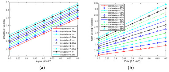
Figure 1. Appliance utility and cost saving functions. (a) $E_{appUtil}$ w.r.t $av{g}_D$; (b) $E_{costSavings}$ w.r.t savings in %.

3.1.2. Cost Saving Function

Consider an appliance scheduling mechanism that gives cost savings of S% with respect to baseline electricity cost, then Equation (8) presents the cost saving function. The value of ζ is to be set by the user within the UCL range in such a way that the remaining portion is allocated to α.

$$\begin{array}{c}\hfill E_{costSavings}=\zeta \ast \frac{S}{100}+\gamma \end{array}$$

(8)

The range of cost savings considering residential EMSs in the literature is between 25% and 75% [19]. This cost saving percentage is measured with respect to the baseline PC cost. Hence, the cost saving range of any EMS under consideration is set between 20% and 70% for this performance metric. Considering an EMS whose savings is lower than 20% or greater than 70% is beyond the scope of the proposed UCL.

Grietus Mulder et al. in [55] presented a near to realistic approach concerning investments made on renewable systems, mainly PV systems and storage devices. Installation cost is one major concern when installing any EMS for an end user. Another variable γ is used that represents $E_{ROI}$ as a part of the savings function. If ROI is expected within one year, the value of γ is set as 0.15. If ROI is expected between one and two years, the value of γ is defined as 0.10, whereas if ROI exceeds two years, the value of γ is set as 0.05.

Figure 1b refers to the cost saving function. In this figure (for simulation purposes), the value of ROI is set as 0.15. Figure 1b states that an EMS that gives financial savings of 70% with respect to bills without EMS, and the value of ζ is set as 0.7, which gives maximum comfort considering the cost saving function.

3.2. Algorithm: UCL

Algorithm 1 depicts the working of the proposed UCL. Values of α and ζ are user defined, such that their sum must yield one, as stated earlier, while the value of γ reflects the UCL gain due to the ROI period and is added in $E_{costSavings}$. Equation (9) is proposed to calculate the UCL of any EMS.

$$\begin{array}{c}\hfill UCL=(\alpha -\frac{\frac{{\sum }_{i=1}^n{D}_{app}}{n}}{T})+(\zeta \ast \frac{s}{100}+\gamma )\end{array}$$

(9)

Algorithm 1 Calculate $UCL=E_{apputil}+E_{costSavings}$.

1: $Savings==x\%$ 2: $ROI==\gamma$ 3: $av{g}_{D}elay==y$ 4: $SchedulingWindow==T$ 5: if $20\le x\le 80$ then 6:   $E_{Savings}\leftarrow \zeta \times \frac{x}{100}$ 7: else 8:   if $20\ge x\ge 80$ then 9:       $E_{Savings}\leftarrow 0$ 10:   end if 11: end if 12: if $\gamma \le 1year$ then 13:   $E_{ROI}\leftarrow \gamma =0.15$ 14:   $E_{costSavings}\leftarrow E_{ROI}+E_{Savings}$ 15: else 16:   if $1year\le \gamma \le$ 2years then 17:       $E_{ROI}\leftarrow \gamma =0.10$ 18:       $E_{costSavings}\leftarrow E_{ROI}+E_{Savings}$ 19:   else 20:       if $\gamma \ge 2year$ then 21:             $E_{ROI}\leftarrow \gamma =0.05$ 22:             $E_{costSavings}\leftarrow E_{ROI}+E_{Savings}$ 23:       end if 24:   end if 25: end if 26: if $0\le y\le 5$ then 27:   $E_{appUtil}\leftarrow \alpha -\frac{y}{T}$ 28:   $UCL=E_{appUtil}+E_{costSavings}$ 29: else 30:   if $y\ge 5$ then 31:       $E_{appUtil}\leftarrow 0$ 32:       $UCL=E_{appUtil}+E_{costSavings}$ 33:   end if 34: end if

4. Basic Building Blocks: EMS

Work on using electricity resourcefully is ongoing in multiple dimensions, and numerous algorithms are used to develop effective EMSs. Optimization techniques and sensor networks are two major dimensions of research in this domain [21]. Considering the existing literature, it can be stated that EMSs are based on a few basic building blocks. These building blocks are listed below in the form of scenarios for energy management solutions.

• Scenario 1: without EMS (baseline model),
• Scenario 2: EMS by using sensors,
• Scenario 3: EMS by using optimization techniques,
• Scenario 4: EMS by using Scenario 2 + Scenario 3,
• Scenario 5: EMS by using storage device + Scenario 3,
• Scenario 6: EMS by using storage device + Scenario 4

Base model and test strategy:

There are N electrical appliances, which are further subdivided into OD and OI appliances, where $P_a$ is the power consumed by an appliance in watts per hour unit, while $P_{OD}$ and $P_{OI}$ represent the power of OD and OI appliances, respectively. Equation (10) gives the per hour power requirement for OD appliances.

$$\begin{array}{c}\hfill P_{OD}=[P_{(1,OD)},P_{(2,OD)},.......P_{(h,OD)}],\forall h=[1,2,3\dots 24],\forall OD\in N\cap OD\end{array}$$

(10)

Equation (11) represents the per hour power requirement for $OI$appliances.

$$\begin{array}{c}\hfill P_{OI}=[P_{(1,OI)},P_{(2,OI)},.......P_{(h,OI)}],\forall h=[1,2,3\dots 24],\forall OI\in N\cap OI\end{array}$$

(11)

$P_{(h,a)}$ represents power usage of an appliance a within hour h out of 24 h of a day. This a belongs to the set of $O{D}_{APP}$, while b belongs to the $O{I}_{APP}$ set, where N is the superset of all appliances, i.e., $N=O{D}_{APP}\cup O{I}_{APP}$. Hourly power demand for $OD$and $OI$ appliances can be expressed in Equations (12) and (13), respectively.

$$\begin{array}{c}\hfill P_{hOD}={\displaystyle \sum _{a=1}^{N\cap OD}}{P}_{h,a}\end{array}$$

(12)

$$\begin{array}{c}\hfill P_{hOI}={\displaystyle \sum _{b=1}^{N\cap OI}}{P}_{h,b}\end{array}$$

(13)

Equation (14) explains the power demand of an hour.

$$\begin{array}{c}\hfill P_h={\displaystyle \sum _{a=1}^{N\cap OD}}{P}_{h,a}+{\displaystyle \sum _{a=1}^{N\cap OI}}{P}_{h,b}\end{array}$$

(14)

Equation (15) states the power demand for 24 h of a day.

$$\begin{array}{c}\hfill P_{T(24)}={\displaystyle \sum _{h=1}^{24}}\left({\displaystyle \sum _{a=1}^{N\cap OD}}{P}_{h,a}+{\displaystyle \sum _{a=1}^{N\cap OI}}{P}_{h,b}\right)\end{array}$$

(15)

In this work, hourly electricity cost is expressed as an array in Equation (16):

$$\begin{array}{c}\hfill C_h=[C_1,C_2,C_3\dots C_h]\forall h=[1,2,3\dots 24]\end{array}$$

(16)

Equation (17) calculates the electricity cost of a day.

$$\begin{array}{c}\hfill C_{t=24}^N={\displaystyle \sum _{a=1}^N\sum _{h=1}^{24}}{P}_{h,allApp}\times C_h\end{array}$$

(17)

Table 3 depicts the assumptions for the simulation setup regarding a list of appliances, their category, the number of operational hours within the 24-h scheduling horizon and power ratings.

Table 3. Baseline data.

Class	Appliance	Opsin T (24 h)	Power (Wph)
$O{D}_{APP}$	Lights	19 h	500
$O{D}_{APP}$	Water Pump	2 h	4000
$O{D}_{APP}$	HVAC	11 h	4000
$O{D}_{APP}$	EWH	3 h	4000
$O{I}_{APP}$	Refrigerator	21 h	3000
$O{I}_{APP}$	Clothes Dryer	2h	2000
$O{I}_{APP}$	Dish Washer	2 h	500
$O{I}_{APP}$	Electric Vehicle	2 h	4000
$O{I}_{APP}$	Washing Machine	2 h	4000

The array expressed in Equation (18) gives the electricity price per unit of each hour within a day. This (assumed as day ahead) hourly cost is utilized in this work for all scenarios.

$$\begin{array}{c}\hfill C_h=[886666666141866614181818181818186]\end{array}$$

(18)

There is an important role of the test bed for any system. Tests are speculated to verify the normal operation of a system, reaching the expectations of the user and the achievement of the expected benefits [9].

To address the complexity of the EMSs, assumptions are made as in Table 3; where the class of the load defines its dependency or independency on human presence inside residential unit. The data presented in Table 3 and the price signal expressed in Equation (18) are kept constant for all scenarios.

4.1. Scenario 1: Without EMS

Scenario 1 is the basic energy consumption pattern of a residential unit and gives a benchmark for comparisons amongst energy management solutions. No effort is made regarding energy or cost reduction, and power is utilized as and when needed. It is obvious that, in this scenario, appliance utility is maximum, while cost savings is totally neglected. Scenario 1 is considered as the test bed for the rest of the five scenarios.

4.2. Scenario 2: EMS by Using Sensors

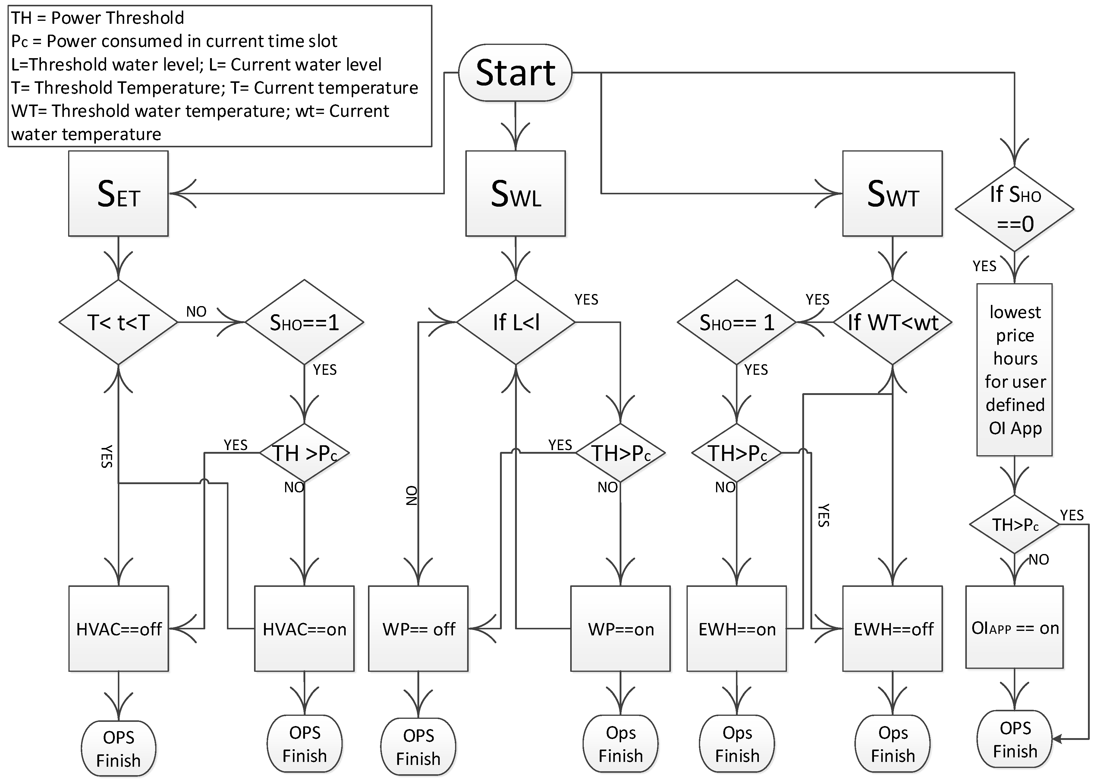
In this scenario, a network of sensors is deployed at the demand side that measures certain attributes. These sensors as programmed to switch on and off appliances after sensing respective features. Figure 2 illustrates the flow diagram of the algorithm, which is used for Scenario 2. Figure 2 reflects the functioning of three basic sensors, i.e., a sensor that senses the environmental temperature ($S_{ET}$) for HVAC, a sensor that senses the water level in the water tank ($S_{WL}$) for the water pump and a sensor that senses the water temperature ($S_{WT}$) for the electric water heater. Besides these basic sensors, one sensor is programmed that reflects the operation of $OI$ appliances that do not require home occupancy. These appliances (OI appliances) are to be scheduled at low-priced hours. Considering appliance-specific sensors, each sensor is programmed to regard, home occupancy, desired ToU range of the appliances and power usage thresholds as explained in [56]. $OI$ appliances are the ones that can be shifted to “low priced” times; while $OD$ appliances are not allowed to run for extra time using the sensor network and user-defined timings/thresholds. As can be seen in Figure 2, before functioning of any appliance, the respective sensed data and thresholds are analyzed. According to these checks, $OD$ appliances are switched on or off.

Figure 2. Flow chart: EMS (Scenario 2).

4.3. Scenario 3: EMS by Using Optimization Techniques

In this scenario, the binary version of the widely-studied PSO, i.e., (BPSO) (considering energy management solutions) is used as in [35,36,57]. Equation (19) expresses the objective function with the respective constraints.

$$obj1=min(C_{t=24}^N)$$

(19)

such that:

$$\begin{array}{}(19\mathrm{a})& \alpha \in (O{D}_{APP}\cup O{I}_{APP})\in N,\hfill (19\mathrm{b})& P{C}_h\le T{h}_h\forall ,T_1=[1,2,3,\dots 24],\hfill (19\mathrm{c})& P{r}_{\beta }^T=(1-\rho )\times P_{\beta }^{max}\forall \beta \in N,and,\forall \beta \notin T_h\hfill \end{array}$$

Constraint “19a” explains that appliance $\alpha \in N$, where $O{D}_{APP}\cup O{I}_{APP}=N$. Constraint “19b” represents the maximum PC value for the current hour to trim PC peaks. $P{r}_{\beta }^T$ represents the probability by which an electrical device $\beta \in N$ can be forced to switch on without following the schedule. Constraint “19c” elaborates the probability of switching on any electrical device without following the schedule made by the scheduler. This is calculated by an update function ρ, whose value is set as binary.

4.4. Scenario 4: EMS by Using Scenario 2 + Scenario 3

In this scenario, EMSs are developed by integrating sensor networks and an evolutionary algorithm as in [56]. Final schedules are made by BPSO on the basis of sensory inputs, while inputs for sensors are user defined. The objective function as in Scenario 3 is utilized here, as well, but with modified constraints. There is also a high impact of the scheduling window size on the appliance utility function [56]. Figure 3 illustrates the basic flow diagram of such a technique that has a scheduling window of 6 h and needs four cycles to complete the 24-h time slot.

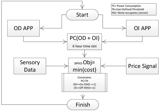
Figure 3. Flow diagram: Scenario 4.

Modifying Equation (17) for four logical scheduling windows, i.e., $T_1$, $T_2$, $T_3$ and $T_4$, Equation (20) is produced for the $T_1$ time slot of 6 h, where $(N-a)$ is the set of appliances that are to be scheduled during this time slot. The set $(N-a)$ is defined by the user and sensory data. The same equation can be used four times to complete one cycle of 24 h, and in each scheduling window, there is a different set of appliances based on the user preferred time and sensor inputs, as can be seen in Equations (20) to (23).

$$\begin{array}{c}\hfill C_{T_1=6}^{N-a}={\displaystyle \sum _{a=1}^{N-a}\sum _{h=1}^6}{P}_{h,a}\times C_h\forall h=1,2,3,4,5,6\end{array}$$

(20)

$$\begin{array}{c}\hfill C_{T_2=6}^{N-b}={\displaystyle \sum _{a=1}^{N-b}\sum _{h=6}^{12}}{P}_{h,a}\times C_h\forall h=6,7,8,9,10,11,12\end{array}$$

(21)

$$\begin{array}{c}\hfill C_{T_3=6}^{N-c}={\displaystyle \sum _{a=1}^{N-c}\sum _{h=12}^{18}}{P}_{h,a}\times C_h\forall h=13,14,15,16,17,18\end{array}$$

(22)

$$\begin{array}{c}\hfill C_{T_4=6}^{N-d}={\displaystyle \sum _{a=1}^{N-d}\sum _{h=18}^{24}}{P}_{h,a}\times C_h\forall h=19,20,21,22,23,24\end{array}$$

(23)

The objective function is set to minimize the cost with given constraints, as presented in Equation (24).

$$obj=min\left((C_{T_1}^{(n-a)})+C_{T_2}^{(n-b)})+C_{T_3}^{(n-c)})+C_{T_4}^{(n-d)}))\right)$$

(24)

Such that:

$$\begin{array}{}(24\mathrm{a})& T^{start}\le U{P}_{\alpha }\le T^{Finish}\forall T=[T_1,T_2,T_3,T_4]\hfill (24\mathrm{b})& U{P}_{(}N-k)\in T\forall T=[T_1,T_2,T_3,T_4]\hfill (24\mathrm{c})& P{C}_h\le T{h}_h\forall T=[T_1,T_2,T_3,T_4],\hfill (24\mathrm{d})& P{r}_x^{T_1}=(1-\rho )\times P_{\alpha }^{max}\forall \alpha \in N,and,\forall \alpha \notin (N-a)\hfill (24\mathrm{e})& P{r}_x^{T_2}=(1-\rho )\times P_{\alpha }^{max}\forall \alpha \in N,and,\forall \alpha \notin (N-b)\hfill (24\mathrm{f})& P{r}_x^{T_3}=(1-\rho )\times P_{\alpha }^{max}\forall \alpha \in N,and,\forall \alpha \notin (N-c)\hfill (24\mathrm{g})& P{r}_x^{T_4}=(1-\rho )\times P_{\alpha }^{max}\forall \alpha \in N,and,\forall \alpha \notin (N-d)\hfill \end{array}$$

Constraint “24a” restricts the use of an appliance within its scheduling horizon. Constraint “24b” states that every set of appliances $(N-k)\in N$ is operational in its corresponding scheduling window. These groups are formed by keeping two inputs, i.e., user preferred ToU and sensed data. Constraint “24c” limits the power usage beyond a threshold value, while the constraints “24d to 24g” express the measure of uncertainty (force starting of any appliance) within any scheduling window.

4.5. Scenario 5: EMS by Using Storage Device + Scenario 3

Investments on RE sources have reached 211 USD since 2004 [58]. There are no such exact figures accessible that presents net worldwide venture made in RE generation; in any case, 15% to 20% of the aggregate power commitment lies in RE sources, as expressed in [59].

Microgrids are gaining attention day by day as a major relief for traditional grid infrastructure. Residential microgrids in support of DSM are studied widely and give optimum cost savings with lowering energy usage from the main grid [60]. The authors in [61] preset an optimal bidding mechanism regarding the day ahead power market in a microgrid environment.

In this scenario, a storage device that is able to store 30% of per day load is added, while load shifting is done by using BPSO. Power is stored in storage devices at off-peak pricing hours and utilized at on-peak pricing hours. This ensures minimal appliance deviation from the desired ToU and is also cost effective.

Algorithm 2 explains the functioning of the energy storage system. The storage device can be in any of the four possible states as fully charged (11), discharging state (10), charging state (01) and idle state (00). B represents the battery; $B_{ch}$ stands for the amount of charge stored in the battery; $Th$ depicts the user-defined per hour PC threshold; while $P{C}_{req}$ gives the PC requirement for this hour.

Algorithm 2 Energy storage system.

1: $B_{idle}$ 2: if $B_{ch}==11$ then 3:   $B\leftarrow 00$ 4: else 5:   if $P{C}_h\le Th$ then 6:       $B\leftarrow 00$ 7:   else 8:       if $P{C}_{req}\ge Th$ && $B_{ch}\ge 60\%$ then 9:             $B\leftarrow 10$ 10:       else 11:             if $B_{ch}\le 30\%$ && $PC\le Th$ then 12:                     $B\leftarrow 01$ 13:             end if 14:       end if 15:   end if 16: end if 17: if $B_{ch}==11$ then 18:   $B\leftarrow 00$ 19: end if

4.6. Scenario 6: EMS by Using Storage Device + Scenario 4

In this scenario, a power storage system (as expressed in Algorithm 2) is combined with the EMS (built on the basis of Scenario 4) to get optimum results. Its installation cost is maximum, but in the long run, this seems to be a vital solution regarding most of the energy problems [33,38,39]. Shortening the logical scheduling window enforces less delay in appliances’ ToU, while integration of an energy storage system helps in normalizing electricity consumption peaks.

5. Results and Discussion

This section presents the numerical results obtained by simulating the proposed UCL and above-mentioned scenarios (in Section 4) reflecting the basic building blocks of energy management solutions. Results regarding Scenario 1 (Section 4.1) are presented in Section 5.2, Scenario 2 (Section 4.2) in Section 5.3, and so on so forth, till Scenario 6 (Section 4.6), whose results are discussed and presented in Section 5.7.

5.1. Numerical Studies: UCL

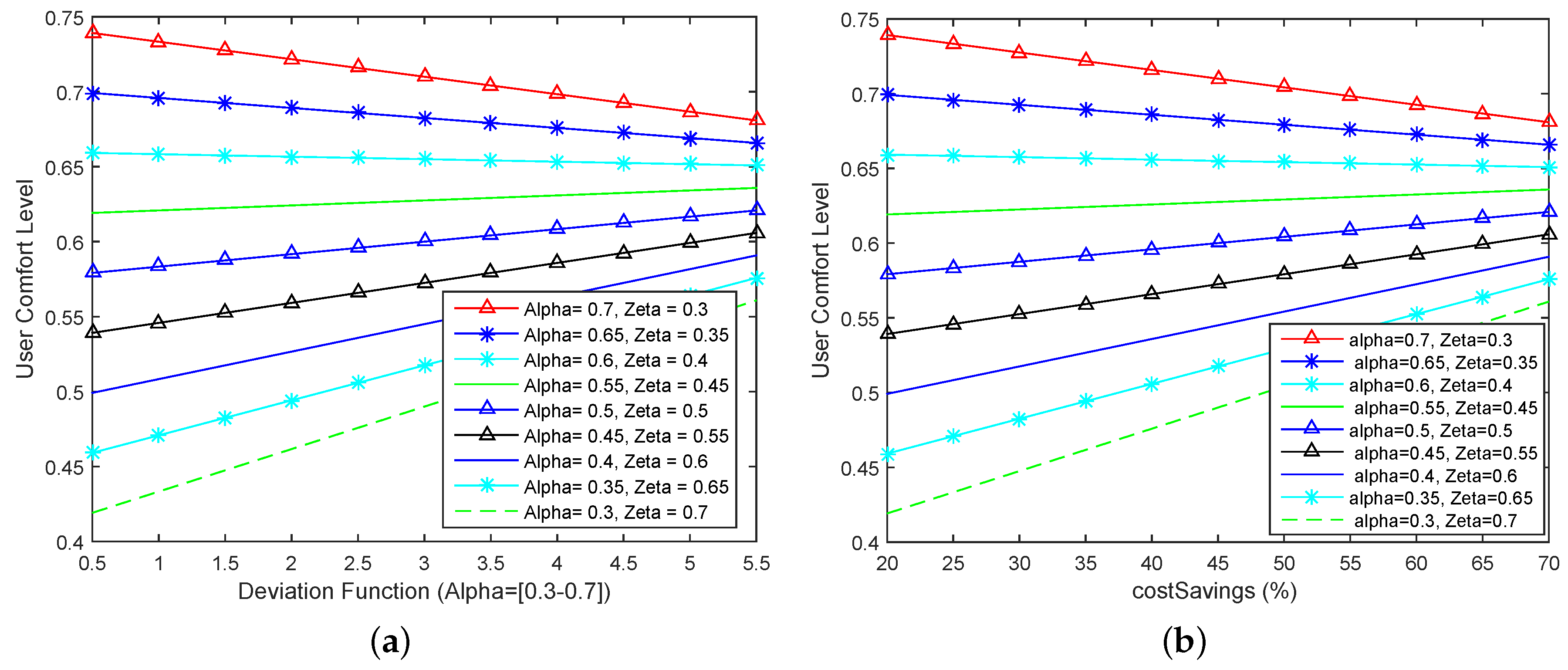
Equation (9), which is depicted in Algorithm 1, is used to compute numerical results with different values of α and ζ. The optimal solution can be achieved (of gaining the highest value of UCL) by keeping $E_{appUtil}$ (Figure 4a) and $E_{costSavings}$ (Figure 4b) variant.

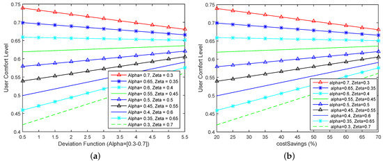
Figure 4. User comfort level keeping $\alpha =$ [0.3–0.7] and $\zeta =$ [0.3–0.7]. (a) $UCL$ w.r.t the appliance utility function; (b) $UCL$ w.r.t the cost saving function.

Table 4 gives UCL values under different situations. By using Equation (9), one can have insight considering the effectiveness of any EMS. This framework helps an end user to select the optimal EMS based on his/her preferences. Hence, it takes a step ahead in minimizing the gap between actual and analytical energy consumption. For example, consider an EMS that gives an average deviation of 1 h with 30% savings. If the user is more cost sensitive and delay-tolerant, then the values of α and ζ will be set as 0.3 and 0.7, respectively. This combination yields UCL of 0.468, which is not very appealing considering user preferences. However, for a delay-intolerant user, where values of α and ζ are set as 0.7 and 0.3, respectively, the EMS (that gives 70% savings and a delay of 1 h) is well suited as it gives the UCL value of 0.748. Hence, a user needs to be clear in his/her preferences regarding energy usage, so that he/she can select an EMS that is able to represent his/her preferences.

Table 4. UCL within different scenarios.

avgD-CSavings	α = 0.3, ζ = 0.7	α = 0.4, ζ = 0.6	α = 0.5, ζ = 0.5	α = 0.6, ζ = 0.4	α = 0.7, ζ = 0.3
1 h-30%	0.468	0.538	0.608	0.678	0.748
2 h-40%	0.496	0.556	0.616	0.676	0.736
3 h-50%	0.525	0.575	0.625	0.675	0.725
4 h-60%	0.553	0.593	0.633	0.673	0.713
5 h-70%	0.581	0.611	0.641	0.671	0.701

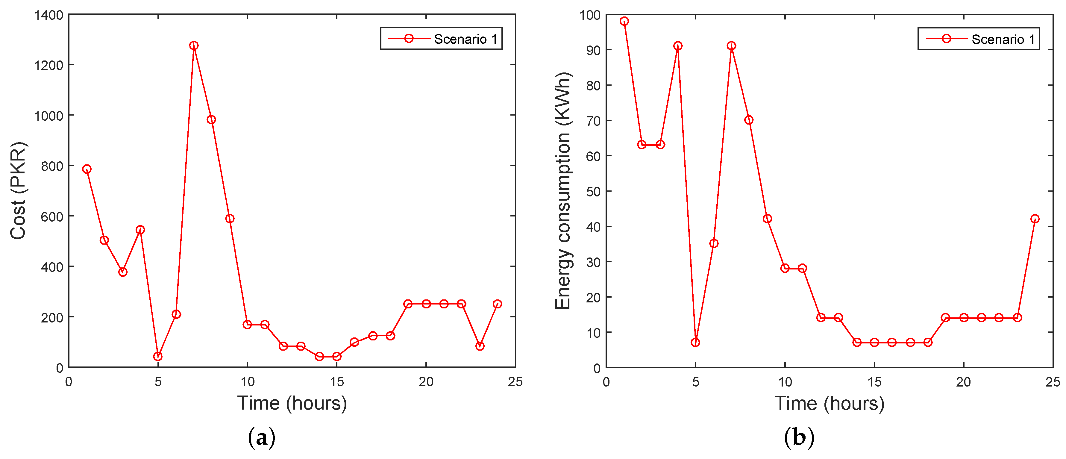
5.2. Scenario 1

Scenario 1 depicts the baseline model as stated earlier. In this scenario, energy is utilized as and when needed without considering the DR program or any other energy management strategy. Figure 5a depicts the cost, while Figure 5b illustrates the load profiles without any EMS.

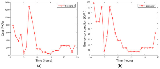
Figure 5. Baseline: without EMS (Scenario 1). (a) Cost profile (Scenario 1); (b) load profile (Scenario 1).

5.3. Scenario 2

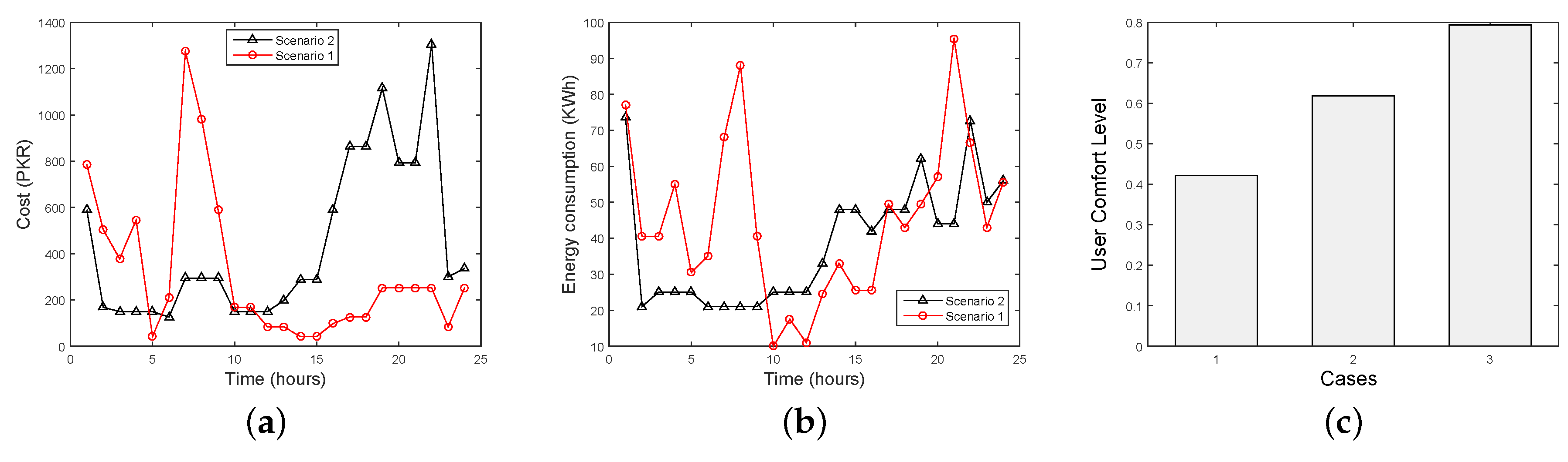
In Scenario 2, a home area sensor network is utilized to control and optimize energy consumption as discussed earlier in Section 4.2. As in accordance with the algorithm illustrated in Figure 3, PC peaks are normalized by using a user-defined power limiter (Figure 6a). Analyzing the cost profile of a week, it can be seen that this scheme rips off the PC peaks; however, it generates one peak during evening hours when the residential unit is fully occupied and the use of electrical appliances is high (Figure 6b).

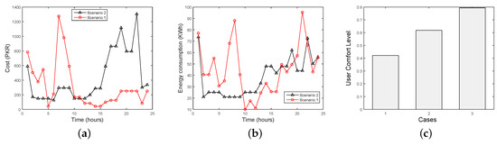
Figure 6. EMS: by using sensor networks (Scenario 2). (a) Cost profile (Scenario 2); (b) load profile (Scenario 2); (c) $UCL$ when: Case 1: $\alpha ,\zeta =0.3,0.7$; Case 2: $\alpha ,\zeta =0.5,0.5$; Case 3: $\alpha ,\zeta =0.7,0.3$.

Considering Figure 6c, UCL values are 0.422, 0.618, 0.794 for Cases 1, 2 and 3, respectively. The value of γ is set as 0.15, as the ROI is expected within a year. Looking carefully, it can be noted that as the value of ζ decreases with respect to α, UCL increases. This explains the inverse relationship between cost savings and lower delay in the ToU of appliances. Overall 15% cost savings was achieved in comparison with the baseline model (Scenario 1), while the average delay is 1 h.

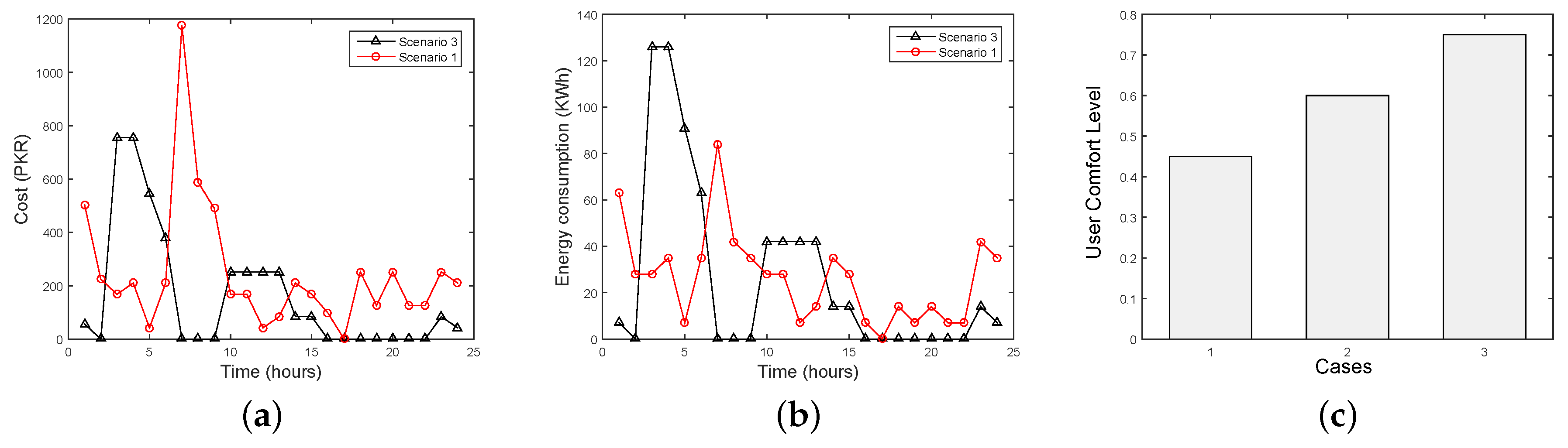
5.4. Scenario 3

In this scenario, load shifting to low priced hours is conducted using BPSO as stated in Section 4.3. Figure 7a illustrates the cost profile of a week. This mechanism shifts the load in a very undesirable manner, as can be seen in Figure 7b. Considering Figure 7c, BPSO gives the maximum value when α is set as 0.7, while ζ is set as 0.3, and γ, which represents the ROI function, is set as 0.10. The total power savings achieved by using BPSO for EMS is 28% with a 3-h (on average) appliance deviation from the desired ToU.

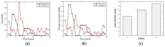
Figure 7. EMS: by using the optimization technique (Scenario 3). (a) Cost profile (Scenario 3); (b) load profile (Scenario 3); (c) $UCL$ when: Case 1: $\alpha ,\zeta =0.3,0.7$; Case 2: $\alpha ,\zeta =0.5,0.5$; Case 3: $\alpha ,\zeta =0.7,0.3$.

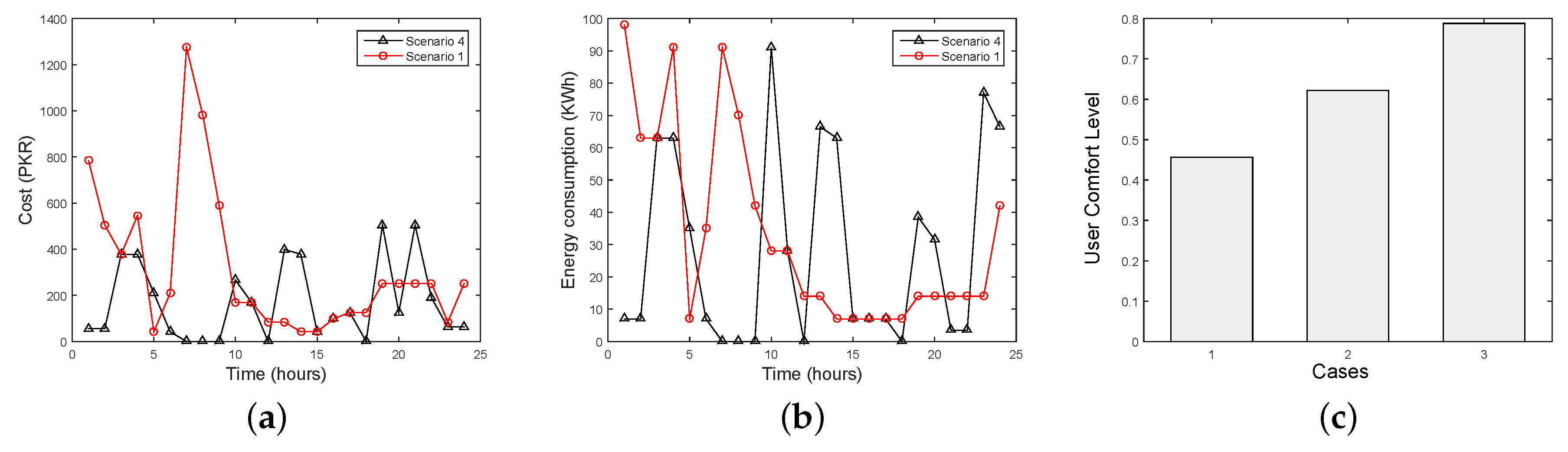
5.5. Scenario 4

As discussed in Section 4.4, this scenario is hybrid in nature, i.e., combining HAN with the optimization technique to optimize energy management. Moreover, dividing 24 h into four logical windows to schedule load results in minimized delay in ToU and maximizes the cost savings. Figure 8a,b illustrates the cost and load profiles of baseline and EMS using Scenario 4, along with numerical values of UCL gain (Figure 8c). Considering the load consumption profile (Figure 8b), there is a peak generated; however, this peak is at a low-priced hour, and its intensity is much lower than the peaks generated in the unscheduled load (Figure 8b). Peaks are normalized, and the load is shifted within its user-defined scheduling window. The value of γ is set at 0.05 as the ROI period exceeds two years; while the deviation in ToU of appliances is calculated as 1.5 h with respect to the desired ToU of an electrical appliance, giving cost savings of 21% with respect to the base model.

Figure 8. EMS: by using a combination of sensors and the evolutionary algorithm (Scenario 4). (a) Cost profile (Scenario 4); (b) load profile (Scenario 4); (c) $UCL$ when: Case 1: $\alpha ,\zeta =0.3,0.7$; Case 2: $\alpha ,\zeta =0.5,0.5$; Case 3: $\alpha ,\zeta =0.7,0.3$.

5.6. Scenario 5

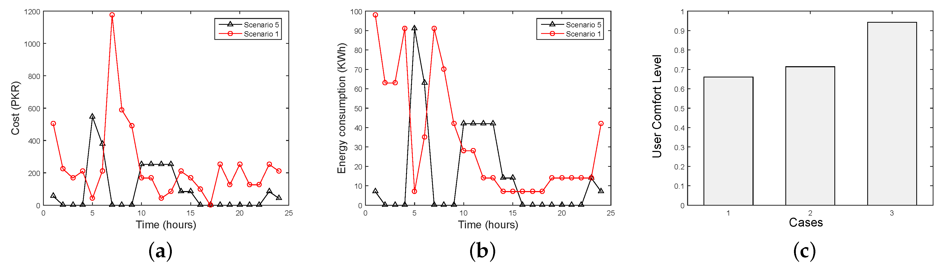
Advancements in storage systems make it more feasible to utilize them in energy management strategies. In this scenario, load shifting is done by utilizing BPSO (Scenario 2), and energy is stored at low-priced hours in the energy storage system as discussed in Section 4.5. This energy is utilized at high-priced hours. Such a mechanism gives more optimum results in terms of cost savings, appliance utility and energy usage times. Figure 9b represents the load profiles with respect to the baseline load. Such mechanisms prove their worth; however, the installation cost is higher. Figure 9c presents the UCL values for three different user requirements.

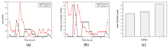
Figure 9. EMS with the combination of the evolutionary algorithm (BPSO) and storage device (Scenario 5). (a) Cost profile (Scenario 5); (b) load profile (Scenario 5); (c) $UCL$ when: Case 1: $\alpha ,\zeta =0.3,0.7$; Case 2: $\alpha ,\zeta =0.5,0.5$; Case 3: $\alpha ,\zeta =0.7,0.3$.

5.7. Scenario 6

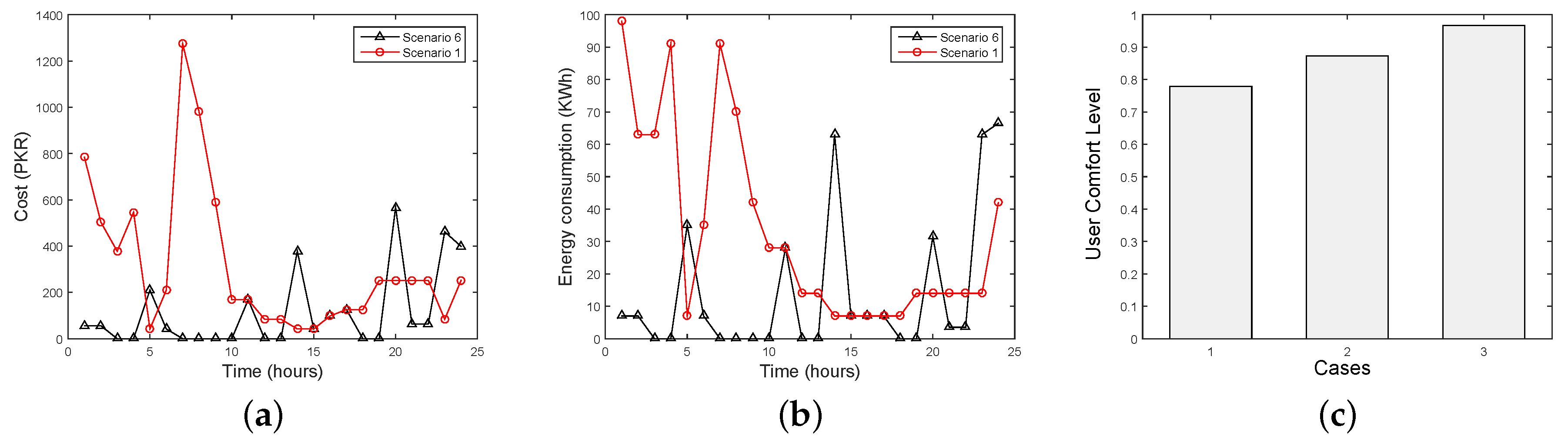
As discussed in Section 4.6, resizing the scheduling window and using BPSO to schedule load in respective time slots ensure less delay, keeping an equilibrium amongst cost and appliance utility, while integration of an energy storage system helps in normalizing electricity consumption peaks, as can be seen in Figure 10a. Load profiles of Scenario 6 and Scenario 1 are presented in Figure 10b. Scenario 6 rips off some PC peaks by using stored electricity. Anticipating Figure 10c, the highest UCL values are achieved in comparison to the above-mentioned scenarios.

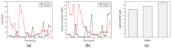
Figure 10. EMS: by using the combination of sensors, the evolutionary algorithm (BPSO) and storage devices (Scenario 6). (a) Cost profile (Scenario 6); (b) load profile (Scenario 6); (c) $UCL$ when: Case 1: $\alpha ,\zeta =0.3,0.7$; Case 2: $\alpha ,\zeta =0.5,0.5$; Case 3: $\alpha ,\zeta =0.7,0.3$.

6. Analysis and Policy Implications

6.1. Energy and Cost Profiles

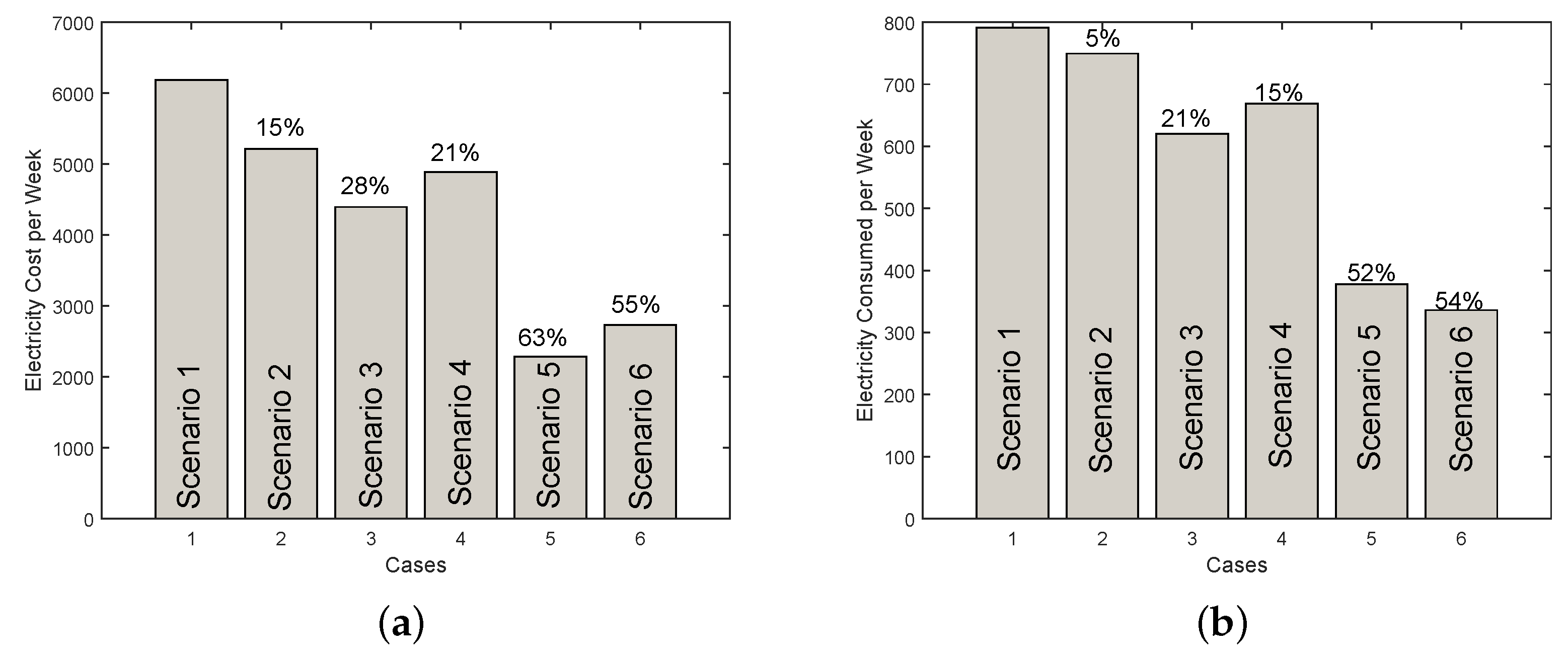
Considering energy profiles (Figure 11b), Scenario 4 utilizes lower energy in comparison with Scenarios 1 and 2; however, considering Scenario 3, it uses more energy. This is due to the integration of the sensor network that maximizes the appliance utility function. Scenario 5, which is a combination of Scenario 3 and a storage system, gives the maximum cost savings of 3906 PKR (63%), 2933 PKR (56%), 2112 PKR (48%), 2604 PKR (53%) and 448 PKR (16%) in comparison to Scenarios 1, 2, 3, 4 and 6, respectively (Figure 11a). Anticipating energy profiles, Scenario 6 proves its worth by utilizing the minimum amount of electricity amongst all other scenarios, as can be seen in Figure 11b.

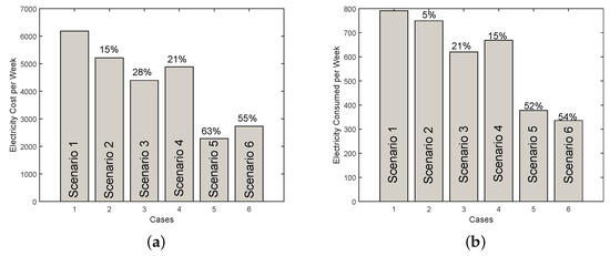
Figure 11. Cost and energy analysis. (a) Cost saving analysis; (b) energy consumption analysis.

Focusing on the impact of γ, Scenario 1 has no installation cost; hence, it has no effect on the performance metric. Deploying an efficient ZigBee or Bluetooth sensor network costs 150,000 PKR to 200,000 PKR, as offered by different vendors. Moreover, such sensors are easily available across the globe. Taking the upper bound of investment, ROI is expected within 205 weeks (more than 3.8 years). Hence, the value of γ is set as 0.05 for Scenario 2. ROI for the remaining scenarios is approximately 139 weeks (2.6 years), 268 weeks (5.5 years), 128 weeks (2.5 years) and 164 weeks (3.1 years) for Scenarios 3, 4, 5 and 6, respectively. In this study, only installation costs were considered, ignoring the element of uncertainty, like currency rate and other market implications.

6.2. UCL and PAR Profiles

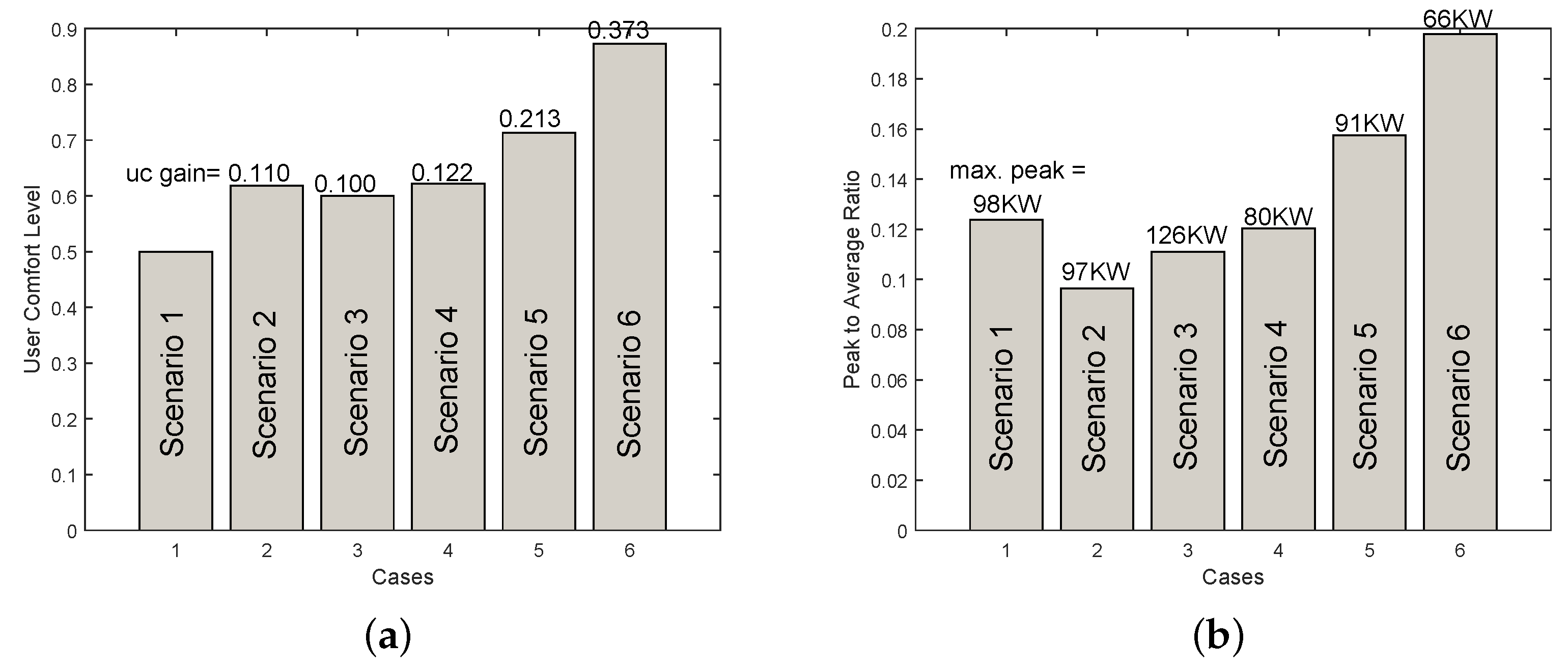
Anticipating UCL(Figure 12a), the values of α (user-defined value of appliance deviation function) and ζ (user-defined value of cost saving function) are set equal to 0.5. These values are user defined and can be changed as per the requirement. Scenario 6 gives the maximum comfort level with the highest installation cost; however, huge cost savings narrow down its ROI period. The UCL gain of 0.373 is achieved in comparison with unscheduled PC as can be seen in Figure 12a. Figure 12b illustrates the value of the highest PC peak and PAR focusing on the six scenarios. Considering Figure 12b, the maximum electrical load utilized by Scenario 1 in a week is 98 KWpHat certain hour, while its PAR is 0.12. The PAR reflecting Scenario 2 is lowest, whereas the PAR of Scenarios 5 and 6 is highest. However, the maximum PC by these two mechanisms is 91 KW and 66 KW, respectively, which is lower than Scenarios 1, 2 and 3. Scenario 3 produces the highest peak, utilizing 126 KWpH, as it tends to shift all load to “low-priced” hours. Scenario 4 takes care of ToU, as well as load shifting for cost savings; hence, it tends to create an equilibrium amongst price and appliance utility. Scenario 4 increased the second lowest PC peak amongst the six scenarios, as can be seen in Figure 12b.

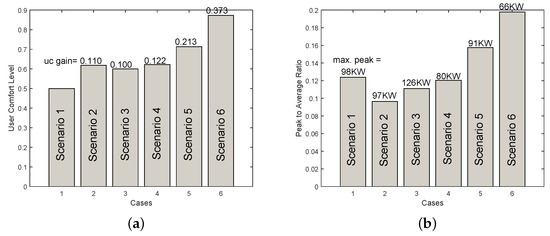
Figure 12. Performance metric and PAR. (a) $UCL$ achieved; (b) PAR.

Table 5 depicts the overall summary of all scenarios that are utilized for developing an EMS.

Table 5. Performance analysis of major EMS mechanisms.

Properties	Scenario 1	Scenario 2	Scenario 3	Scenario 4	Scenario 5	Scenario 6
Scheduling Window	No window	no window	1 × 24 = 24 h	4 × 6 = 24 h	1 × 24 =24 h	4 × 6 = 24 h
Power limiting threshold	No	Constant	Fixed	Dynamic range	Fixed	Dynamic range
Appliance categorization	No	No	Based on PC	Based on HO	Based on PC	Based on HO and PC
Load balancing	No	Yes	Load shift	w.r.t. need and price	Power bank	Balance between cost and price
Appliance utility	Maximum	Maximum	Do not care	Tends to create equilibrium	Do not care	optimum
Shave cost peaks	No	Yes	Yes	Yes	Yes	Yes
User comfort level	Compromised	Compromised	Compromised	Achieve a level of user satisfaction	better	Maximum
Home occupancy considered	Yes	Yes	No	Yes	No	Yes
Take care of utility	No	To some extent	Only at user premises	Tends to accommodate	Yes	Yes
Computational cost	No	Minimum complexity	Yes	Yes	Yes	Maximum complexity

6.3. UCL Scope and Limitations

The basic goals of EMSs are to reduce electricity bills for the end users and avoid PC peaks for the utility companies. By achieving these targets, numerous problems are addressed, the most important of which are the reduction in carbon emissions and utilizing fossil fuels resourcefully.

This study offers the optimal EMS selection framework for any PC unit considering user comfort and preferences. As discussed earlier, user comfort or user convenience tends to reduce the difference between estimated and actual PC. An EMS that gives a greater comfort level lessens this difference. Hence, a performance metric is formulated in this work that is able to predict the performance of any EMS prior to its installation anticipating user preferences. However, the proposed UCL has certain limitations. UCL is limited to the study of various EMSs proposed in the literature that reflect power usage and bill reduction to a certain level, where the grid is the only power source, or at the maximum small-scale PV, or the energy storage system is employed, which is able to manage 30% of the total power requirement of a day. This power storage is charged at low-priced hours of the day. Heavy storage devices and MGs that can support a residential unit to reach islanded mode are beyond the scope of this study. Market fluctuations are not controllable; hence, investment costs may vary that directly influence the value of γ. Moreover, an EMS that saves cost below 20% or above 70% is out of scope considering the proposed performance metric.

There is one critical aspect in using UCL, i.e., the electricity user must be aware of the relationship between cost savings and delay in the ToU of appliances, which are inversely proportional to each other. Hence, the user must decide the values of α and ζ carefully to achieve the maximum level of satisfaction. Moreover, the electricity user must be aware of his/her baseline electricity consumption and bills paid to the utility for comparison purposes. Hence, users have a responsibility to determine their preferences realistically with respect to appliance utility and savings to minimize the gap between estimated and actual PC, as well as cost savings.

7. Conclusions

Utilizing power resourcefully is the need of this era for preserving the atmosphere (limiting carbon emissions) and natural resources (fossil fuel consumption). To reach optimality in energy consumption, numerous EMSs are developed under the umbrella of DR programs. Diverse load shifting and load-preserving techniques have been proposed since last decade. However, there is a wide gap between actual and analytical results. The basic properties of existing EMSs are bill reduction, appliance deviation in ToU and ROI period. In this work, a numerical solution was proposed, which is based on the user-defined proportion of appliance deviation and cost savings, whereas the ROI period is dependent on the investment made and savings. By using the proposed metric (UCL), a user can choose an EMS that not only enhances comfort level, but is also cost and energy effective. This also tends to minimize the gap between the analytical and actual results of EMSs. In the latter part of paper, an extended literature analysis is presented that depicts the major techniques used in developing an EMS. EMSs are based on five generic building blocks, which were demonstrated and simulated (in the form of five scenarios) for performance analysis keeping the proposed UCL as the performance metric.

For the developing part of the world, differences between power demand and supply can be observed. Hence, energy management solutions are a must for such parts of the globe. However, lack of awareness, accessibility of smart appliances and economic issues result in poor energy managing strategies. Applying Scenario 2 (EMS using sensor networks) is advocated, which not only gives minimum PAR, but it is also an easily available and affordable to preserve electricity and ensure user comfort at a good level.

References

- Energy Information Administration. International Energy Outlook 2016, U.S. Department of Energy. May 2016. Available online: http://www.eia.gov/outlooks/ieo/pdf/0484(2016).pdf (accessed on 7 March 2017). [Google Scholar]
- Cetin, K.S.; Tabares-Velasco, P.C.; Novoselac, A. Appliance daily energy use in new residential buildings: Use profiles and variation in time-of-use. Energy Build. 2014, 84, 716–726. [Google Scholar] [CrossRef]
- Alam, M.R.; Reaz, M.B.; Ali, M.A. A review of smart homes—Past, present, and future. IEEE Trans. Syst. Man Cybern. Part C (Appl. Rev.) 2012, 42, 1190–1203. [Google Scholar] [CrossRef]
- Abushnaf, J.; Rassau, A.; Górnisiewicz, W. Impact of dynamic energy pricing schemes on a novel multi-user home energy management system. Electr. Power Syst. Res. 2015, 125, 124–132. [Google Scholar] [CrossRef]
- Bera, S.; Gupta, P.; Misra, S. D2S: Dynamic demand scheduling in smart grid using optimal portfolio selection strategy. IEEE Trans. Smart Grid 2015, 6, 1434–1442. [Google Scholar] [CrossRef]
- Taniguchi, T.; Kawasaki, K.; Fukui, Y.; Yano, S. Automated Linear Function Submission-based Double Auction for Emergent Real-Time Pricing in a Regional Smart Grid. 2015. Available online: http://arxiv.org/abs/1503.06408v1 (accessed on 2 January 2016).
- Mahmood, A.; Javaid, N.; Khan, M.A.; Razzaq, S. An overview of load management techniques in smart grid. Int. J. Energy Res. 2015, 39, 1437–1450. [Google Scholar] [CrossRef]
- Graditi, G.; Ippolito, M.G.; Telaretti, E.; Zizzo, G. Technical and economical assessment of distributed electrochemical storages for load shifting applications: An Italian case study. Renew. Sustain. Energy Rev. 2016, 57, 515–523. [Google Scholar] [CrossRef]
- Siano, P.; Graditi, G.; Atrigna, M.; Piccolo, A. Designing and testing decision support and energy management systems for smart homes. J. Ambient Intell. Humaniz. Comput. 2013, 4, 651–661. [Google Scholar] [CrossRef]
- Zheng, M.; Meinrenken, C.J.; Lackner, K.S. Agent-based model for electricity consumption and storage to evaluate economic viability of tariff arbitrage for residential sector demand response. Appl. Energy 2014, 126, 297–306. [Google Scholar] [CrossRef]
- Graditi, G.; Ippolito, M.G.; Lamedica, R.; Piccolo, A.; Ruvio, A.; Santini, E.; Siano, P.; Zizzo, G. Innovative control logics for a rational utilization of electric loads and air-conditioning systems in a residential building. Energy Build. 2015, 102, 1–7. [Google Scholar] [CrossRef]
- Qela, B.; Mouftah, H.T. Observe, learn, and adapt (OLA)—An algorithm for energy management in smart homes using wireless sensors and artificial intelligence. IEEE Trans. Smart Grid 2012, 3, 2262–2272. [Google Scholar] [CrossRef]
- Auger, A.; Doerr, B. Theory of Randomized Search Heuristics: Foundations and Recent Developments; World Scientific: Singapore, 2011. [Google Scholar]
- Hrovatin, N.; Dolšak, N.; Zorić, J. Factors impacting investments in energy efficiency and clean technologies: Empirical evidence from Slovenian manufacturing firms. J. Clean. Prod. 2016, 127, 475–486. [Google Scholar] [CrossRef]
- Menezes, A.C.; Cripps, A.; Bouchlaghem, D.; Buswell, R. Predicted vs. actual energy performance of non-domestic buildings: Using post-occupancy evaluation data to reduce the performance gap. Appl. Energy 2012, 97, 355–364. [Google Scholar] [CrossRef]
- USGBC Research Committee. A National Green Building Research Agenda. US Green Building Council, 2007. Available online: http://www.usgbc.org/Docs/Archive/General/Docs3402.pdf (accessed on 15 March 2014).
- De Wilde, P. The gap between predicted and measured energy performance of buildings: A framework for investigation. Autom. Constr. 2014, 41, 40–49. [Google Scholar] [CrossRef]
- Kibert, C.J. Sustainable Construction: Green Building Design and Delivery; John Wiley & Sons: New York, NY, USA, 2016. [Google Scholar]
- Dwaikat, L.N.; Ali, K.N. Measuring the Actual Energy Cost Performance of Green Buildings: A Test of the Earned Value Management Approach. Energies 2016, 9, 188. [Google Scholar] [CrossRef]
- Andreadou, N.; Guardiola, M.O.; Fulli, G. Telecommunication Technologies for Smart Grid Projects with Focus on Smart Metering Applications. Energies 2016, 9, 375. [Google Scholar] [CrossRef]
- Lobaccaro, G.; Carlucci, S.; Löfström, E. A Review of Systems and Technologies for Smart Homes and Smart Grids. Energies 2016, 9, 348. [Google Scholar] [CrossRef]
- Thomas, B.L.; Cook, D.J. Activity-Aware Energy-Efficient Automation of Smart Buildings. Energies 2016, 9, 624. [Google Scholar] [CrossRef]
- Kan, E.M.; Kan, S.L.; Ling, N.H.; Soh, Y.; Lai, M. Multi-zone Building Control System for Energy and Comfort Management. In Hybrid Intelligent Systems; Springer: Berlin, Germany, 2016; pp. 41–51. [Google Scholar]
- Cetin, K.S.; Manuel, L.; Novoselac, A. Thermal comfort evaluation for mechanically conditioned buildings using response surfaces in an uncertainty analysis framework. Sci. Technol. Built Environ. 2016, 22, 140–152. [Google Scholar] [CrossRef]
- Mendes, T.D.; Godina, R.; Rodrigues, E.M.; Matias, J.C.; Catalão, J.P. Smart home communication technologies and applications: Wireless protocol assessment for home area network resources. Energies 2015, 8, 7279–7311. [Google Scholar] [CrossRef]
- Ikpehai, A.; Adebisi, B.; Rabie, K.M.; Haggar, R.; Baker, M. Experimental Study of 6LoPLC for Home Energy Management Systems. Energies 2016, 9, 1046. [Google Scholar] [CrossRef]
- Faria, P.; Vale, Z.; Baptista, J. Constrained consumption shifting management in the distributed energy resources scheduling considering demand response. Energy Convers. Manag. 2015, 93, 309–320. [Google Scholar] [CrossRef]
- Pallonetto, F.; Oxizidis, S.; Milano, F.; Finn, D. The effect of time-of-use tariffs on the demand response flexibility of an all-electric smart-grid-ready dwelling. Energy Build. 2016, 128, 56–67. [Google Scholar] [CrossRef]
- Castillo-Cagigal, M.; Matallanas, E.; Gutiérrez, A.; Monasterio-Huelin, F.; Caamaño-Martín, E.; Masa-Bote, D.; Jiménez-Leube, J. Heterogeneous collaborative sensor network for electrical management of an automated house with PV energy. Sensors 2011, 11, 11544–11559. [Google Scholar] [CrossRef] [PubMed]
- Gao, B.; Zhang, W.; Tang, Y.; Hu, M.; Zhu, M.; Zhan, H. Game-theoretic energy management for residential users with dischargeable plug-in electric vehicles. Energies 2014, 7, 7499–7518. [Google Scholar] [CrossRef]
- Wang, Z.; Yang, R.; Wang, L. Intelligent multi-agent control for integrated building and micro-grid systems. In Proceedings of the 2011 IEEE PES Innovative Smart Grid Technologies (ISGT), Anaheim, CA, USA, 17–19 January 2011; pp. 1–7.
- Shaikh, P.H.; Nor, N.B.; Nallagownden, P.; Elamvazuthi, I.; Ibrahim, T. Intelligent multi-objective control and management for smart energy efficient buildings. Int. J. Electr. Power Energy Syst. 2016, 74, 403–409. [Google Scholar] [CrossRef]
- Lin, W.M.; Tu, C.S.; Tsai, M.T. Energy management strategy for microgrids by using enhanced bee colony optimization. Energies 2015, 9, 5. [Google Scholar] [CrossRef]
- Kim, H.Y.; Kang, H.J. A Study on Development of a Cost Optimal and Energy Saving Building Model: Focused on Industrial Building. Energies 2016, 9, 181. [Google Scholar] [CrossRef]
- Huang, Y.; Tian, H.; Wang, L. Demand response for home energy management system. Int. J. Electr. Power Energy Syst. 2015, 73, 448–455. [Google Scholar] [CrossRef]
- Bradac, Z.; Kaczmarczyk, V.; Fiedler, P. Optimal scheduling of domestic appliances via MILP. Energies 2014, 8, 217–232. [Google Scholar] [CrossRef]
- Rasheed, M.B.; Javaid, N.; Ahmad, A.; Khan, Z.A.; Qasim, U.; Alrajeh, N. An Efficient Power Scheduling Scheme for Residential Load Management in Smart Homes. Appl. Sci. 2015, 5, 1134–1163. [Google Scholar] [CrossRef]
- Iwafune, Y.; Ikegami, T.; da Silva Fonseca, J.G.; Oozeki, T.; Ogimoto, K. Cooperative home energy management using batteries for a photovoltaic system considering the diversity of households. Energy Convers. Manag. 2015, 96, 322–329. [Google Scholar] [CrossRef]
- Zhang, D.; Evangelisti, S.; Lettieri, P.; Papageorgiou, L.G. Economic and environmental scheduling of smart homes with microgrid: DER operation and electrical tasks. Energy Convers. Manag. 2016, 110, 113–124. [Google Scholar] [CrossRef]
- Karimi-Nasab, M.; Modarres, M.; Seyedhoseini, S.M. A self-adaptive PSO for joint lot sizing and job shop scheduling with compressible process times. Appl. Soft Comput. 2015, 27, 137–147. [Google Scholar] [CrossRef]
- Adika, C.O.; Wang, L. Autonomous appliance scheduling for household energy management. IEEE Trans. Smart Grid 2014, 5, 673–682. [Google Scholar] [CrossRef]
- Polaki, S.K.; Reza, M.; Roy, D.S. A genetic algorithm for optimal power scheduling for residential energy management. In Proceedings of the 2015 IEEE 15th International Conference on Environment and Electrical Engineering (EEEIC), Florence, Italy, 10–13 June 2015; pp. 2061–2065.
- Haider, H.T.; See, O.H.; Elmenreich, W. Dynamic residential load scheduling based on adaptive consumption level pricing scheme. Electr. Power Syst. Res. 2016, 133, 27–35. [Google Scholar] [CrossRef]
- Khan, M.A.; Javaid, N.; Mahmood, A.; Khan, Z.A.; Alrajeh, N. A generic demand-side management model for smart grid. Int. J. Energy Res. 2015, 39, 954–964. [Google Scholar] [CrossRef]
- Jaffe, A.B.; Stavins, R.N. The energy-efficiency gap What does it mean? Energy Policy 1994, 22, 804–810. [Google Scholar] [CrossRef]
- Sunikka-Blank, M.; Galvin, R. Introducing the prebound effect: the gap between performance and actual energy consumption. Build. Res. Inf. 2012, 40, 260–273. [Google Scholar] [CrossRef]
- Pusnik, M.; Al-Mansour, F.; Sucic, B.; Gubina, A.F. Gap analysis of industrial energy management systems in Slovenia. Energy. 2016, 108, 41–49. [Google Scholar] [CrossRef]
- Schulze, M.; Nehler, H.; Ottosson, M.; Thollander, P. Energy management in industry–a systematic review of previous findings and an integrative conceptual framework. J. Clean. Prod. 2016, 112, 3692–3708. [Google Scholar] [CrossRef]
- Cetin, K.S.; Manuel, L.; Novoselac, A. Effect of technology-enabled time-of-use energy pricing on thermal comfort and energy use in mechanically-conditioned residential buildings in cooling dominated climates. Build. Environ. 2016, 96, 118–130. [Google Scholar] [CrossRef]
- Toftum, J.; Kazanci, O.B.; Olesen, B.W. Effect of Set-point Variation on Thermal Comfort and Energy Use in a Plus-energy Dwelling. In Proceedings of the 9th Windsor Conference: Making Comfort Relevant, Windsor, UK, 7–10 April 2016.
- Salehi, M.M.; Cavka, B.T.; Frisque, A.; Whitehead, D.; Bushe, W.K. A case study: The energy performance gap of the Center for Interactive Research on Sustainability at the University of British Columbia. J. Build. Eng. 2015, 4, 127–139. [Google Scholar] [CrossRef]
- Mahmood, D.; Javaid, N.; Nouman, U.; Urrahman, A.; Khan, Z.A.; Qasim, U. Comparative Analysis of Energy Management Solutions focusing Practical Implementation. In Proceedings of the 2016 10th International Conference on Complex, Intelligent, and Software Intensive Systems (CISIS), Fukuoka, Japan, 6–8 July 2016; pp. 271–277.
- Zhou, B.; Li, W.; Chan, K.W.; Cao, Y.; Kuang, Y.; Liu, X.; Wang, X. Smart home energy management systems: Concept, configurations, and scheduling strategies. Renew. Sustain. Energy Rev. 2016, 61, 30–40. [Google Scholar] [CrossRef]
- Paradiso, F.; Paganelli, F.; Giuli, D.; Capobianco, S. Context-Based Energy Disaggregation in Smart Homes. Future Internet 2016, 8, 4. [Google Scholar] [CrossRef]
- Mulder, G.; Six, D.; Claessens, B.; Broes, T.; Omar, N.; Van Mierlo, J. The dimensioning of PV-battery systems depending on the incentive and selling price conditions. Appl. Energy 2013, 111, 1126–1135. [Google Scholar] [CrossRef]
- Mahmood, D.; Javaid, N.; Alrajeh, N.; Khan, Z.A.; Qasim, U.; Ahmed, I.; Ilahi, M. Realistic Scheduling Mechanism for Smart Homes. Energies 2016, 9, 202. [Google Scholar] [CrossRef]
- Liu, Z.; Chen, C.; Yuan, J. Hybrid Energy Scheduling in a Renewable Micro Grid. Appl. Sci. 2015, 5, 516–531. [Google Scholar] [CrossRef]
- UNEP BN. Global Trends in Renewable Energy Investments 2011. Analysis of Trends and Issues in the Financing of Renewable Energy. 2011. [Google Scholar]
- OECD/IEA. International Energy Agency—Scenarios & Strategies to 2050. 2010. Available online: https://www.iea.org/publications/freepublications/publication/etp2010.pdf (accessed on 7 March 2017).
- Ferruzzi, G.; Graditi, G.; Rossi, F.; Russo, A. Optimal operation of a residential microgrid: The role of demand side management. Intell. Ind. Syst. 2015, 1, 61–82. [Google Scholar] [CrossRef]
- Ferruzzi, G.; Cervone, G.; Delle Monache, L.; Graditi, G.; Jacobone, F. Optimal bidding in a Day-Ahead energy market for Micro Grid under uncertainty in renewable energy production. Energy 2016, 106, 194–202. [Google Scholar] [CrossRef]
© 2017 by the authors. Licensee MDPI, Basel, Switzerland. This article is an open access article distributed under the terms and conditions of the Creative Commons Attribution (CC BY) license ( http://creativecommons.org/licenses/by/4.0/).