Optimal Scheduling of Microgrid with Multiple Distributed Resources Using Interval Optimization

Abstract

In this paper, an optimal day-ahead scheduling problem is studied for a microgrid with multiple distributed resources. For the sake of coping with the prediction uncertainties of renewable energies and loads and taking advantage of the time-of-use price for buying/selling electricity, an interval-based optimization model for maximum profits is developed. To reduce the computational complexity in solving the model, the possibility degree comparison between an interval and a real number is used to convert the interval constraints into the general ones; meanwhile, some slack variables and complementary conditions are introduced to eliminate the absolute-value operation. Unlike the stochastic optimization, the interval optimization only needs the upper-lower bounds of the uncertain variables instead of their probability distribution functions, which is beneficial to the practical application. Furthermore, the possible profit interval and the expected optimal profit can be determined by solving the optimization model. Numerical simulations are performed on a microgrid system modified from the benchmark low voltage network in the European Union project “Microgrid”, and the results demonstrate the effectiveness of the proposed method.

1. Introduction

In recent years, the application of microgrids in power system has drawn growing attention. A microgrid is characterized by flexibility, intelligence and compatibility. It is not only able to integrate the small-scale distributed renewable resources, but also helps to enhance the reliability and efficiency of the power system [1]. There are two operation modes for the microgrid, namely grid-connected mode and islanded mode [2,3]. In the grid-connected mode, the microgrid usually provides ancillary service to the main power grid. In the islanded mode, the microgrid needs to keep the supply-demand balance by itself.

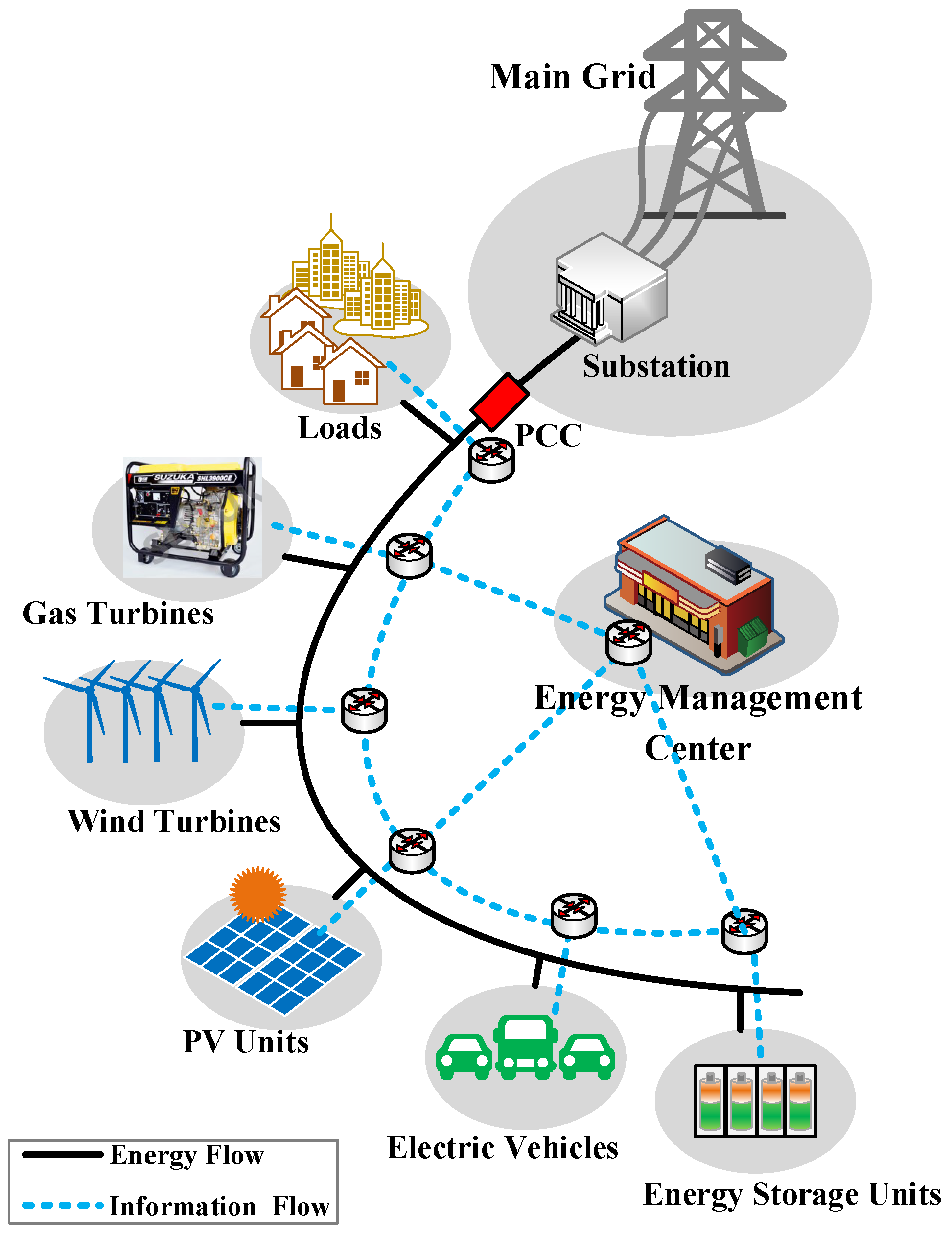
It is assumed that a microgrid comprises wind turbines (WTs), photovoltaic units (PVs) and gas turbines (GTs), energy storage units (ESUs), electric vehicles (EVs) and loads (see Figure 1). In order to provide high-quality and economical electricity, the microgrid operation needs to be scheduled reasonably [4]. As the brain of the microgrid, the energy management system (EMS) takes charge of coordinating the output power of the distributed resources and the exchanged power with the main grid to minimize the operational cost or maximize the total profits, according to the information from load prediction, power prediction of renewable energy and electricity price [5,6,7]. As far as the architecture of EMS is concerned, there exist three kinds of structures: the centralized structure [8], the hierarchical structure [7,9] and the distributed structure [5,10]. The authors in [11] give a comprehensive review about the EMS of microgrids and summarize the recent state of the art in control structures, strategies and technologies for the multi-time-scale energy management of microgrids.

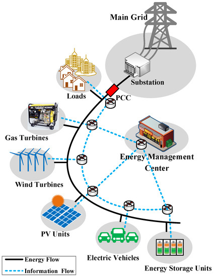
Figure 1. Configuration of a microgrid.

Power generation scheduling in the EMS plays an important role in the microgrid operation, which is used to dispatch various energy resources to meet the load demands at the minimum cost subject to the physical constraints of the microgrid [12]. Generally speaking, the power generation scheduling of the microgrid involves economic dispatch (ED) and optimal power flow (OPF). In essence, both the ED and the OPF can be boiled down to the optimization issue.

In the past ten years, the optimization issue of the microgrid has been investigated by many researchers. In [13], the authors present an optimization algorithm to minimize the total cost of buying power from multiple generations under the microgrid framework. In [14], an optimization procedure is developed to make a schedule for the distributed generators and the storage in the microgrid to minimize the operating cost and the pollutant emission. For multiple interconnected microgrids, the authors in [15] propose a pricing mechanism based on the potential game theory to study the anticipated benefits in an open market. Considering the users’ thermal comfort and the system constraints, the authors in [16] propose an optimal day-ahead price-based power scheduling scheme for a community-scale microgrid for the purpose of maximizing the expected benefit and minimizing the operational cost. For a multi-microgrid interconnected system, the authors in [7] present a two-level hierarchical optimization method. Under the hierarchical framework, the lower level and the upper level are responsible for an individual microgrid and the entire system, respectively. In [17], the authors propose a hierarchical decision-making framework for a distribution company and a microgrid to optimize their respective objective in a cooperative manner. It should be noted that the uncertainties of renewable energies in microgrids have not been considered in the aforementioned works.

Comparing with the conventional power systems, more uncertainties will be confronted in the generation scheduling of a microgrid due to less accuracy in the prediction of small-scale renewable energies and load demands [12,18]. Recently, some researchers have studied the problems about the generation scheduling of microgrids considering the prediction uncertainties. Their works can be categorized into stochastic optimization, fuzzy optimization, robust optimization and interval optimization.

For the stochastic optimization for microgrid operation, some research works have been done in recent years. In [19], the authors develop a cuckoo optimization algorithm to solve the stochastic unit commitment problem of microgrids. In [20], the availability of distributed generators, energy storage units and responsive loads are studied through analyzing their uncertainty natures, and then, a stochastic optimization method based on Monte Carlo simulation is used to cope with the uncertainties. For a typical microgrid with a diesel generator, renewable energies and energy storage, the authors in [21] present a probabilistic constrained approach to model the uncertainties of load and renewable power predictions and use stochastic dynamic programming to find the optimal day-ahead scheduling of the microgrid. In [22], a hierarchical stochastic control scheme is proposed to coordinate the charging power of the plug-in electric vehicles and the wind power. In this scheme, the truncated Gaussian distribution is used to describe the uncertainty of wind power prediction. In [23], the authors model the forecast errors of wind speed and solar irradiance using the probability distribution functions and then take the Latin hypercube sampling to generate the possible scenarios of renewable generation for day-head energy and reserve scheduling. It is known that the stochastic optimization approach relies on the accurate probability distribution functions of the uncertain variables. However, it is difficult for us to obtain the accurate probability distributions.

In fuzzy optimization methods, fuzzy variables are used to describe the uncertainties of optimization model, fuzzy sets are composed of all of the uncertain constraints, and the degree to meet constraints is defined as the membership function [24]. Recently, the fuzzy optimization methods have been applied to microgrid scheduling preliminarily. For instance, the authors in [25] present a fuzzy-logic expert system to handle uncertainties related to the forecasted parameters and the fuzzy operational environment of the microgrid. In the context of multi-objective optimization of the microgrid, the authors in [26] propose a fuzzy decision approach to represent microgrid operators’ preferences in compromising between two objectives. As far as the fuzzy optimization methods are concerned, the fuzzy membership functions of the uncertainties often have some subjective arbitrariness since they are determined by decision-maker’s personal experience [27].

To enhance the robustness of the generation scheduling, some researchers have studied several robust optimization methods. Considering the prediction errors of energy generation and consumption in a long time scale, the authors in [28] present a robust multi-objective scheduling approach for dispatching distributed energy resources in the microgrid. In [29], the authors present a robust optimization method to deal with the uncertainty of wind power output and provide a robust unit commitment schedule in the day-ahead market. The authors in [30] propose a robust distributed economic dispatch approach for a grid-connected microgrid with high-penetration renewable energy and optimize the worst-case transaction cost stemming from the uncertainties of the renewable energy. In [31], the authors present a multi-level robust optimization model for an energy-intensive corporate microgrid to minimize the unbalance cost in the worst case considering the uncertainties of loads. To save the cost and reduce the emission, the authors in [32] develop a multi-objective robust planning approach for the microgrid with the consideration of multiple uncertainties during operation, for the purpose of calculating the worst-case cost among possible scenarios. The authors in [33] develop a robust EMS for a microgrid under the mathematical framework of model predictive control, in which a fuzzy prediction interval model is used to describe the uncertainties of the renewable energy sources. Though the robust optimization methods do not require the explicit probability distribution functions of the uncertain variables, the obtained generation scheduling strategy tends to be conservative.

As we know, it is easier in practice to determine the upper and lower bounds of an uncertain variable than to obtain its probability distribution function. Mathematically, an interval is usually used to describe an uncertain variable whose upper-lower bounds are known [34,35]. Recently, the interval optimization for the generation scheduling of power system has drawn increasing attention. For example, the authors in [36,37] present an interval-based optimization method to solve the unit commitment problem of the power system considering the uncertainties of distributed energy resources and loads. The authors in [38] adopt intervals to describe the uncertainty of load prediction in the linear economic dispatch model and then formulate the optimistic and pessimistic solution. In [39], the authors propose an improved interval optimization method based on differential evolution for dynamic economic dispatch to minimize the economic and environmental costs of a microgrid. Comparing robust optimization with interval optimization, we can draw the differences between them. The robust optimization is to achieve the optimal decision under the worst case of uncertain parameters. Therefore, the solution of the robust optimization has good robustness against uncertainties, but it has much conservativeness, as well. The interval optimization uses the intervals to describe the uncertain parameters in objective function and constraints. The solution of the interval optimization is related to the possibility degree that the interval constraints are satisfied. In general, the bigger the possibility degree the decision-maker chooses for the constraints, the better the robustness of the solution the decision-maker obtains, but the more conservativeness the decision-maker needs to bear, and vice versa. In comparison with the robust optimization, the interval optimization is very flexible, though it has some subjectivity.

This paper focuses on the optimal day-ahead scheduling problem for a microgrid with multiple distributed energy resources. The optimization objective is to maximize the profits of the microgrid operation by scheduling the active and reactive power of all of the controllable energy resources under the time-of-use price mechanism. In the optimization model, the uncertainties of renewable resource prediction and load prediction are modeled by using intervals. Meanwhile, a set of interval decision variables (active and reactive power output of a gas turbine) are designed to balance the fluctuations of the renewable energies in the microgrid. To facilitate solving the optimization model, the possibility degree comparison between an interval and a real number is adopted to simplify the objective function and the constraints. In addition, some slack variables and complementary conditions are introduced to eliminate the absolute-value function (ABS function). The solution of the optimization problem in this paper provides a schedule for the active and reactive power output of all of the controllable energy resources, as well as the possible profit interval and the expected optimal profit of the microgrid.

The rest of this paper is organized as follows. Section 2 formulates a day-ahead scheduling model for the microgrid in which the interval variables are used to describe the uncertainties of the renewable resource and load prediction. In Section 3, the mathematical transformations are adopted to eliminate the ABS functions and the interval variables of the scheduling model for reducing the model complexity. In Section 4, the case studies on a typical microgrid are presented to demonstrate the effectiveness of the proposed method. Section 5 draws the conclusions of this paper.

2. Scheduling Problem Formulation

This paper considers a kind of microgrid consisting of gas turbines (GTs), photovoltaic units (PVs), wind turbines (WTs), energy storage units (ESUs), electric vehicles (EVs) and a number of loads. For the microgrid, the power predictions of PVs and WTs have inevitable uncertainties, since the power of PVs and WTs is subject to the local weather conditions, such as irradiance, temperature and wind speed [40]. In addition, load prediction is also inaccurate due to the randomness in load demand.

In this paper, intervals are adopted to describe the prediction values with uncertainties for PV power, WT power and load power, i.e.,

$$\begin{array}{c}{P}_{\mathrm{wt},w}^{\mathcal{I}}(t)=[P_{\mathrm{wt},w}^{\mathcal{L}}(t),P_{\mathrm{wt},w}^{\mathcal{R}}(t)]\hfill \\ P_{\mathrm{pv},v}^{\mathcal{I}}(t)=[P_{\mathrm{pv},v}^{\mathcal{L}}(t),P_{\mathrm{pv},v}^{\mathcal{R}}(t)]\hfill \\ P_{\mathrm{load},i}^{\mathcal{I}}(t)=[P_{\mathrm{load},i}^{\mathcal{L}}(t),P_{\mathrm{load},i}^{\mathcal{R}}(t)]\hfill \\ Q_{\mathrm{load},i}^{\mathcal{I}}(t)=[Q_{\mathrm{load},i}^{\mathcal{L}}(t),Q_{\mathrm{load},i}^{\mathcal{R}}(t)]\hfill \end{array}$$

(1)

where the superscripts $\mathcal{I}$, $\mathcal{L}$ and $\mathcal{R}$ denote an interval, left bound and right bound of the corresponding power prediction, respectively. Generally, it is easy for us to determine the left bound and right bound of the prediction interval by analyzing the historical predicted data and real data. Therefore, it is assumed in this paper that the bounds of the above prediction intervals in (1) have been known in advance.

According to the power balance requirements of the microgrid, the power output of the controllable distributed resources should vary in a certain range to counteract the uncertainties of the PV power, WT power and loads. Here, the power outputs of GTs are selected to take the counteracting responsibility. Thus, the active power and the reactive power of a GT are designed to be two interval variables, i.e.,

$$\begin{array}{c}{P}_{\mathrm{gt},g}^{\mathcal{I}}(t)=[P_{\mathrm{gt},g}^{\mathcal{L}}(t),P_{\mathrm{gt},g}^{\mathcal{R}}(t)]\hfill \\ Q_{\mathrm{gt},g}^{\mathcal{I}}(t)=[Q_{\mathrm{gt},g}^{\mathcal{L}}(t),Q_{\mathrm{gt},g}^{\mathcal{R}}(t)]\hfill \end{array}$$

(2)

where $P_{\mathrm{gt},g}^{\mathcal{I}}(t)$ and $Q_{\mathrm{gt},g}^{\mathcal{I}}(t)$ denote the active and reactive power intervals of the GT, respectively. It should be noted that the power intervals $P_{\mathrm{gt},g}^{\mathcal{I}}(t)$ and $Q_{\mathrm{gt},g}^{\mathcal{I}}(t)$ serve as decision variables, not uncertain parameters.

2.1. Objective Function

This paper concerns the grid-connected microgrid, which allows bidirectional power flow at the point of common coupling (PCC). This means that the microgrid operator is permitted to buy the short electricity from (or sell the spare electricity to) the main grid at any time. The objective of power generation scheduling can be to maximize the benefits or minimize the cost. Here, we take the maximum profits as the objective of the power generation scheduling for the microgrid.

Generally, the profits of the microgrid are equal to the total earnings minus the total costs. The objective function for the generation scheduling of the microgrid is formulated as:

$$maxF={\displaystyle \sum _{t=1}^T}\left[F_{\mathrm{E}}(t)-F_{\mathrm{C}}(t)\right]$$

(3)

where $F_{\mathrm{E}}(t)$ and $F_{\mathrm{C}}(t)$ denote the earnings and costs of the microgrid in the $t-\mathrm{th}$ time interval (1 h for each time interval), respectively; T denotes the number of time intervals.

The earnings $F_{\mathrm{E}}(t)$ are calculated by:

$$\begin{array}{c}{F}_{\mathrm{E}}(t)={\gamma }_{\mathrm{s}}(t)P_{\mathrm{pcc}}^{\mathrm{s}}(t)+{\gamma }_{\mathrm{b}}(t){\displaystyle \sum _{i=1}^{\mathcal{N}}}{P}_{\mathrm{load},i}^{\mathcal{I}}(t)+{\gamma }_{\mathrm{sub}}(t)[{\displaystyle \sum _{p=1}^{\mathcal{P}}}{P}_{\mathrm{pv},p}^{\mathcal{I}}(t)+{\displaystyle \sum _{w=1}^{\mathcal{W}}}{P}_{\mathrm{wt},w}^{\mathcal{I}}(t)]\hfill \end{array}$$

(4)

where ${\gamma }_{\mathrm{s}}$ is the selling price; ${\gamma }_{\mathrm{b}}$ is the buying price; ${\gamma }_{\mathrm{sub}}$ is the subsidy price from the government; $P_{\mathrm{pcc}}^{\mathrm{s}}(t)$ is the power, which is sold to the main grid; $\mathcal{P}$ is the number of PVs; $\mathcal{W}$ is the number of WTs.

The costs $F_{\mathrm{C}}(t)$ are calculated by:

$$\begin{array}{c}{F}_{\mathrm{C}}(t)={\gamma }_{\mathrm{b}}(t)P_{\mathrm{pcc}}^{\mathrm{b}}(t)+{\gamma }_{\mathrm{b}}(t)P_{\mathrm{loss}}(t)+F_{\mathrm{C},\mathrm{gt}}(t)+F_{\mathrm{C},\mathrm{esu}}(t)+F_{\mathrm{C},\mathrm{ev}}(t)\hfill \end{array}$$

(5)

where $P_{\mathrm{pcc}}^{\mathrm{b}}(t)$ is the power, which is bought from the main grid; $P_{\mathrm{loss}}(t)$ is the total power loss of microgrid; $F_{\mathrm{C},\mathrm{gt}}(t)$ is the total cost of GTs; $F_{\mathrm{C},\mathrm{esu}}(t)$ is the total cost of ESUs; $F_{\mathrm{C},\mathrm{ev}}(t)$ is the total cost of EVs.

As we know, for a grid-connected microgrid, selling electricity to the main power grid and buying electricity from the main power grid cannot occur at the same time. Therefore, to avoid this phenomenon appearing in the objective function, the sold power and the bought power at the $t-\mathrm{th}$ time interval can be expressed as follows:

$$\begin{array}{c}{P}_{\mathrm{pcc}}^{\mathrm{s}}(t)=\frac{|P_{\mathrm{pcc}}(t)|-P_{\mathrm{pcc}}(t)}{2}\hfill \\ P_{\mathrm{pcc}}^{\mathrm{b}}(t)=\frac{\mid P_{\mathrm{pcc}}(t)\mid +P_{\mathrm{pcc}}(t)}{2}\hfill \end{array}$$

(6)

where $P_{\mathrm{pcc}}(t)$ denotes the actual power at the PCC (the direction of power flow is from the main grid to the microgrid). Obviously, $P_{\mathrm{pcc}}(t)<0$ implies the selling-electricity transaction, otherwise implying the buying-electricity transaction.

For the microgrid with $\mathcal{N}$ buses, the total active power loss is calculated as follows [41]:

$$\begin{array}{c}{P}_{\mathrm{loss}}\left(t\right)=\frac{1}{2}{\displaystyle \sum _{i=1}^{\mathcal{N}}}{\displaystyle \sum _{j=1}^{\mathcal{N}}}{R}_{ij}(G_{ij}^2+B_{ij}^2)\left[V_i^2(t)+V_j^2(t)-2V_i(t)V_j(t)cos{\theta }_{ij}(t)\right]\hfill \end{array}$$

(7)

where $V_i(t)$ and $V_j(t)$ denote the voltage at bus i and bus j, respectively; ${\theta }_{ij}(t)={\theta }_i(t)-{\theta }_j(t)$ denotes the phase difference between bus i and bus j; $G_{ij}$ and $B_{ij}$ are the real component and the imaginary component of the complex admittance matrix elements $[Y_{ij}]\in {\mathbb{C}}^{\mathcal{N}\times \mathcal{N}}$, respectively; $R_{ij}$ is the resistance of the line between bus i and bus j.

Assuming that the operational cost of a GT is proportional to the active power output, then the total costs of all of the GTs can be calculated by:

$$F_{\mathrm{C},\mathrm{gt}}(t)={\displaystyle \sum _{g=1}^{\mathcal{G}}}{\gamma }_{\mathrm{gt},g}{P}_{\mathrm{gt},g}^{\mathcal{I}}(t)$$

(8)

where $P_{\mathrm{gt},g}^{\mathcal{I}}(t)$ and ${\gamma }_{\mathrm{gt},g}$ are the active power interval and the cost coefficient of the g-th GT, respectively; $\mathcal{G}$ is the number of GTs.

The operational cost of an ESU is mainly related to the charging times of its storage battery. The cost of an ESU for per charging/discharging cycle can be calculated by:

$$c_{\mathrm{esu},s}=\frac{C_{\mathrm{esu},s}^{\mathrm{inv}}}{K_{\mathrm{esu},s}}$$

(9)

where $C_{\mathrm{esu},s}^{\mathrm{inv}}$ is the investment cost for the s-th ESU and $K_{\mathrm{esu},s}$ is the total charging/discharging cycles. In the t-th time interval, the total operational cost of all of the ESUs can be calculated by:

$$\begin{array}{c}{F}_{\mathrm{C},\mathrm{esu}}(t)=\frac{1}{2}{\displaystyle \sum _{s=1}^{\mathcal{S}}}{c}_{\mathrm{esu},s}\frac{|P_{\mathrm{esu},s}(t)|}{E_{\mathrm{esu},s}^{\mathrm{rate}}}={\displaystyle \sum _{s=1}^S}{\gamma }_{\mathrm{esu},s}|P_{\mathrm{esu},s}(t)|\hfill \end{array}$$

(10)

where ${\gamma }_{\mathrm{esu},s}=c_{\mathrm{esu},s}/(2E_{\mathrm{esu},s}^{\mathrm{rate}})$; $P_{\mathrm{esu},s}(t)$ and $E_{\mathrm{esu},s}^{\mathrm{rate}}$ are the active power and the rated capacity of the s-th ESU, respectively; $\mathcal{S}$ is the number of ESUs.

Similarly, the total operational cost of all of the EVs in the t-th time interval is:

$$\begin{array}{c}{F}_{\mathrm{C},\mathrm{ev}}(t)=\frac{1}{2}{\displaystyle \sum _{v=1}^{\mathcal{V}}}{c}_{\mathrm{ev},v}\frac{|P_{\mathrm{ev},v}(t)|}{E_{\mathrm{ev},v}^{\mathrm{rate}}}={\displaystyle \sum _{v=1}^{\mathcal{V}}}{\gamma }_{\mathrm{ev},v}|P_{\mathrm{ev},v}(t)|\hfill \end{array}$$

(11)

where ${\gamma }_{\mathrm{ev},v}=c_{\mathrm{ev},v}/(2E_{\mathrm{ev},v}^{\mathrm{rate}})$; $P_{\mathrm{ev},v}(t)$ and $E_{\mathrm{ev},v}^{\mathrm{rate}}$ are the active power and the rated capacity of the v-th EV, respectively; $\mathcal{V}$ is the number of EVs.

2.2. Operational Constraints

The optimal generation scheduling of microgrid operation is to maximize the profits on the premise that all of the operational constraints of the system are satisfied.

2.2.1. Constraints of Power Flow Balance

The microgrid operation needs to meet the power flow constraints. The power flow equations at the i-th bus are given as follows [42]:

$$\begin{array}{c}\hfill P_i(t)=V_i(t){\displaystyle \sum _{j=1}^{\mathcal{N}}}{V}_j(t)\left[G_{ij}cos{\theta }_{ij}(t)+B_{ij}sin{\theta }_{ij}(t)\right]\\ \hfill Q_i(t)=V_i(t){\displaystyle \sum _{j=1}^{\mathcal{N}}}{V}_j(t)\left[G_{ij}sin{\theta }_{ij}(t)-B_{ij}cos{\theta }_{ij}(t)\right]\end{array}$$

(12)

where $G_{ij}$ and $B_{ij}$ are the real component and the imaginary component of the complex admittance matrix elements $[Y_{ij}]\in {\mathbb{C}}^{\mathcal{N}\times \mathcal{N}}$. $P_i(t)$ and $Q_i(t)$ are the injected active and reactive power at bus i, respectively, which can be expressed as follows:

$$\begin{array}{c}{P}_i\left(t\right)=P_{\mathrm{esu},i}(t)+P_{\mathrm{ev},i}(t)+P_{\mathrm{pcc},i}(t)+P_{\mathrm{gt},i}^{\mathcal{I}}(t)+P_{\mathrm{wt},i}^{\mathcal{I}}(t)+P_{\mathrm{pv},i}^{\mathcal{I}}(t)-P_{\mathrm{load},i}^{\mathcal{I}}(t)\hfill \\ Q_i\left(t\right)=Q_{\mathrm{esu},i}(t)+Q_{\mathrm{ev},i}(t)+Q_{\mathrm{pcc},i}(t)+Q_{\mathrm{gt},i}^{\mathcal{I}}(t)+Q_{\mathrm{wt},i}(t)+Q_{\mathrm{pv},i}(t)-Q_{\mathrm{load},i}^{\mathcal{I}}(t)\hfill \end{array}$$

(13)

where $P_{\mathrm{pcc},i}(t)$, $P_{\mathrm{gt},i}^{\mathcal{I}}(t)$, $P_{\mathrm{wt},i}^{\mathcal{I}}(t)$, $P_{\mathrm{pv},i}^{\mathcal{I}}(t)$, $P_{\mathrm{esu},i}(t)$, $P_{\mathrm{ev},i}(t)$ and $P_{\mathrm{load},i}^{\mathcal{I}}(t)$ denote the active power outputs of PCC, GTs, WTs, PVs, ESUs, EVs and loads at bus i, respectively; $Q_{\mathrm{pcc},i}(t)$, $Q_{\mathrm{gt},i}^{\mathcal{I}}(t)$, $Q_{\mathrm{wt},i}(t)$, $Q_{\mathrm{pv},i}(t)$, $Q_{\mathrm{esu},i}(t)$, $Q_{\mathrm{ev},i}(t)$ and $Q_{\mathrm{load},i}^{\mathcal{I}}(t)$ denote the reactive powers of PCC, GTs, WTs, PVs, ESUs, EVs and loads at bus i, respectively.

2.2.2. Constraints of Bus Voltage

The voltage at each bus is required not to exceed the prescribed bounds. Therefore, the constraint of voltage at bus i is given by the following inequality:

$$V_i^{min}\le V_i(t)\le V_i^{max}$$

(14)

where $V_i^{min}$ and $V_i^{max}$ are the lower bound and the upper bound, respectively.

2.2.3. Constraints of Power Exchange at PCC

The exchanged active and reactive power between the microgrid and the main grid at PCC need to meet the following constraints:

$$\begin{array}{c}{P}_{\mathrm{pcc}}^{min}\le P_{\mathrm{pcc}}(t)\le P_{\mathrm{pcc}}^{max}\hfill \\ Q_{\mathrm{pcc}}^{min}\le Q_{\mathrm{pcc}}(t)\le Q_{\mathrm{pcc}}^{max}\hfill \end{array}$$

(15)

where $P_{\mathrm{pcc}}^{min}$, $P_{\mathrm{pcc}}^{max}$, $Q_{\mathrm{pcc}}^{min}$ and $Q_{\mathrm{pcc}}^{max}$ denote the minimum and maximum values of the exchanged active and reactive power at PCC, respectively.

2.2.4. Constraints of WTs and PVs

The constraints for the reactive power of WT and PV are given as follows:

$$\begin{array}{c}{Q}_{\mathrm{wt},w}^{min}\le Q_{\mathrm{wt},w}(t)\le Q_{\mathrm{wt},w}^{max}\hfill \\ Q_{\mathrm{pv},p}^{min}\le Q_{\mathrm{pv},p}(t)\le Q_{\mathrm{pv},p}^{max}\hfill \end{array}$$

(16)

where $Q_{\mathrm{wt},w}^{min}$, $Q_{\mathrm{wt},w}^{max}$, $Q_{\mathrm{pv},p}^{min}$ and $Q_{\mathrm{pv},p}^{max}$ denote the minimum and maximum values of the reactive power of the w-th WT and the p-th PV, respectively.

2.2.5. Constraints of GTs

The constraints for the active and reactive power outputs of the g-th GT are given as follows:

$$\begin{array}{c}{P}_{\mathrm{gt},g}^{min}\le P_{\mathrm{gt},g}^{\mathcal{I}}(t)\le P_{\mathrm{gt},g}^{max}\hfill \\ Q_{\mathrm{gt},g}^{min}\le Q_{\mathrm{gt},g}^{\mathcal{I}}(t)\le Q_{\mathrm{gt},g}^{max}\hfill \end{array}$$

(17)

where $P_{\mathrm{gt},g}^{min}$, $P_{\mathrm{gt},g}^{max}$, $Q_{\mathrm{gt},g}^{min}$, and $Q_{\mathrm{gt},g}^{max}$ denote the minimum and maximum values of the active and reactive power of the g-th GT, respectively.

2.2.6. Constraints of ESUs

The ESU operation is required to meet the following constraints:

$$P_{\mathrm{esu},s}^{min}\le P_{\mathrm{esu},s}(t)\le P_{\mathrm{esu},s}^{max}$$

(18)

$$Q_{\mathrm{esu},s}^{min}\le Q_{\mathrm{esu},s}(t)\le Q_{\mathrm{esu},s}^{max}$$

(19)

$$E_{\mathrm{esu},s}^{min}\le E_{\mathrm{esu},s}(t)\le E_{\mathrm{esu},s}^{max}$$

(20)

$$E_{\mathrm{esu},s}(t)=E_{\mathrm{esu},s}(t-1)-P_{\mathrm{esu},s}(t)$$

(21)

$$E_{\mathrm{esu},s}(0)=E_{\mathrm{esu},s}(T)$$

(22)

where the inequalities (18)–(20) represent constraints of the active power capacity, reactive power capacity and energy capacity of the ESU, respectively; the equality (21) denotes the charging/discharging energy balance; the equality (22) denotes the energy balance between the initial and the final state of charge (SoC). $P_{\mathrm{esu},s}^{min}$ and $P_{\mathrm{esu},s}^{max}$ denote the minimum and the maximum values of the active power of the s-th ESU, respectively; $Q_{\mathrm{esu},s}^{min}$ and $Q_{\mathrm{esu},s}^{max}$ denote the minimum and the maximum values of the reactive power of the s-th ESU, respectively; $E_{\mathrm{esu},s}^{min}$ and $E_{\mathrm{esu},s}^{max}$ denote the minimum and the maximum values of the energy of the s-th ESU, respectively.

2.2.7. Constraints of EVs

For the vehicle-to-grid EVs, at the grid-connected time, the operational constraints are similar to the ones of the ESUs, i.e.,

$$P_{\mathrm{ev},v}^{min}\le P_{\mathrm{ev},v}(t)\le P_{\mathrm{ev},v}^{max},t\in T_{\mathrm{ev}}$$

(23)

$$Q_{\mathrm{ev},v}^{min}\le Q_{\mathrm{ev},v}(t)\le Q_{\mathrm{ev},v}^{max},t\in T_{\mathrm{ev}}$$

(24)

$$E_{\mathrm{ev},v}^{min}\le E_{\mathrm{ev},v}(t)\le E_{\mathrm{ev},v}^{max},t\in T_{\mathrm{ev}}$$

(25)

$$E_{\mathrm{ev},v}(t)=E_{\mathrm{ev},v}(t-1)-P_{\mathrm{ev},v}(t),t\in T_{\mathrm{ev}}$$

(26)

$$E_{\mathrm{ev},v}(0)=E_{\mathrm{ev},v}(T)$$

(27)

where $T_{\mathrm{ev}}$ denotes the set of all of the grid-connected time intervals.

To satisfy the traveling requirements in the morning and afternoon, the energy of EVs should be adequate for departing from and returning to the charging station. Therefore, at the departing time, the energy of EVs should meet the minimum energy constraints:

$$\begin{array}{c}{E}_{\mathrm{ev},\mathrm{dep},v}^{min}\le E_{\mathrm{ev},v}(t_{\mathrm{mor},\mathrm{dep}})\hfill \\ E_{\mathrm{ev},\mathrm{dep},v}^{min}\le E_{\mathrm{ev},v}(t_{\mathrm{aft},\mathrm{dep}})\hfill \end{array}$$

(28)

where $E_{\mathrm{ev},\mathrm{dep},v}^{min}$ denotes the required minimum energy for the v-th EV traveling; $t_{\mathrm{mor},\mathrm{dep}}$ and $t_{\mathrm{aft},\mathrm{dep}}$ denote the departing time in the morning and afternoon, respectively.

Assuming that the EV returns to the charging station after k hours, the residual energy of the EV at the returning time can be calculated by:

$$\begin{array}{c}{E}_{\mathrm{ev},v}(t_{\mathrm{mor},\mathrm{ret}})=E_{\mathrm{ev},v}(t_{\mathrm{mor},\mathrm{dep}})-k{P}_{\mathrm{ev}}^{\mathrm{av}}\hfill \\ E_{\mathrm{ev},v}(t_{\mathrm{aft},\mathrm{ret}})=E_{\mathrm{ev},v}(t_{\mathrm{aft},\mathrm{dep}})-k{P}_{\mathrm{ev}}^{\mathrm{av}}\hfill \end{array}$$

(29)

where $P_{\mathrm{ev}}^{\mathrm{av}}$ denotes the average traveling power of each EV; $t_{\mathrm{mor},\mathrm{ret}}$ and $t_{\mathrm{aft},\mathrm{ret}}$ denote the returning time in the morning and afternoon, respectively.

By combining the above objective function and constraints, we obtain the day-ahead scheduling model of the microgrid operation. In the scheduling model, there exist some interval variables and ABS functions, which increase the complexity of the model.

3. Scheduling Model Transformation

The scheduling model of the microgrid includes the ABS functions, the interval objective function and the interval constraints. As we know, the ABS functions consume much of the calculation resource, and the interval constraints cause many difficulties in solving the model. To simplify the scheduling model, this paper adopts mathematical transformations to eliminate the ABS functions and the interval variables.

3.1. Transformation for Interval Constraints and the Objective Function

3.1.1. Arithmetic Operations between Intervals

An interval is defined to be a set consisting of random variables with the left and right limits, i.e.,

$$A^{\mathcal{I}}=[A^{\mathcal{L}},A^{\mathcal{R}}]=\{a:A^{\mathcal{L}}\le a\le A^{\mathcal{R}}\}$$

(30)

Alternatively, the interval $A^{\mathcal{I}}$ can also be represented by midpoint and width, i.e.,

$$A^{\mathcal{I}}=⟨m(A^{\mathcal{I}}),w(A^{\mathcal{I}})⟩$$

(31)

where $m(A^{\mathcal{I}})$ and $w(A^{\mathcal{I}})$ represent the midpoint and width of the interval $A^{\mathcal{I}}$, respectively, which can be expressed as follows:

$$\begin{array}{c}m(A^{\mathcal{I}})=(A^{\mathcal{R}}+A^{\mathcal{L}})/2\hfill \\ w(A^{\mathcal{I}})=(A^{\mathcal{R}}-A^{\mathcal{L}})/2\hfill \end{array}$$

(32)

Assuming that a constant λ and two interval numbers ($A^{\mathcal{I}}$ and $B^{\mathcal{I}}$) are given, the operation rules for scalar multiplication, addition and subtraction are defined as follows [43,44]:

$$\lambda ·A^{\mathcal{I}}=\left\{\begin{array}{c}\left[\lambda A^{\mathcal{L}},\lambda A^{\mathcal{R}}\right]\mathrm{if}\lambda \ge 0\\ \left[\lambda A^{\mathcal{R}},\lambda A^{\mathcal{L}}\right]\mathrm{if}\lambda <0\end{array}\right.$$

(33)

$$\lambda +A^{\mathcal{I}}=\left[\lambda +A^{\mathcal{L}},\lambda +A^{\mathcal{R}}\right]$$

(34)

$$A^{\mathcal{I}}+B^{\mathcal{I}}=\left[A^{\mathcal{L}}+B^{\mathcal{L}},A^{\mathcal{R}}+B^{\mathcal{R}}\right]$$

(35)

$$A^{\mathcal{I}}-B^{\mathcal{I}}=\left[A^{\mathcal{L}}-B^{\mathcal{R}},A^{\mathcal{R}}-B^{\mathcal{L}}\right]$$

(36)

$$m(A^{\mathcal{I}}+B^{\mathcal{I}})=m(A^{\mathcal{I}})+m(B^{\mathcal{I}})$$

(37)

$$m(A^{\mathcal{I}}-B^{\mathcal{I}})=m(A^{\mathcal{I}})-m(B^{\mathcal{I}})$$

(38)

$$w(A^{\mathcal{I}}+B^{\mathcal{I}})=w(A^{\mathcal{I}}-B^{\mathcal{I}})=w(A^{\mathcal{I}})+w(B^{\mathcal{I}})$$

(39)

3.1.2. Definition of Possibility Degree

In interval mathematics, there are two kinds of comparisons: $A^{\mathcal{I}}\le B^{\mathcal{I}}$ and $A^{\mathcal{I}}\le b$ (b is a real number). It should be noted that $A^{\mathcal{I}}\le B^{\mathcal{I}}$ does not mean $B^{\mathcal{I}}$ is larger than $A^{\mathcal{I}}$ as the comparison between two real numbers; rather, it denotes that $B^{\mathcal{I}}$ is superior to $A^{\mathcal{I}}$. In interval optimization theory, the possibility degree is often used to describe the degree to which an interval is superior to another interval [35]. The meanings of $A^{\mathcal{I}}\le b$ are similar to those of $A^{\mathcal{I}}\le B^{\mathcal{I}}$. Considering that the interval constraints in the scheduling model are related to the comparison between an interval and a real number, we next introduce the possibility degree definition for $A^{\mathcal{I}}\le b$.

The geometric relation between an interval $A^{\mathcal{I}}$ and a real number b is shown in Figure 2. On the basis of the position relation shown in Figure 2a–c, the possibility degree for $A^{\mathcal{I}}\le b$ is defined as follows [35]:

$$P\{A^{\mathcal{I}}\le b\}=\left\{\begin{array}{c}0\mathrm{for}{A}^{\mathcal{L}}>b\hfill \\ \frac{b-A^{\mathcal{L}}}{A^{\mathcal{R}}-A^{\mathcal{L}}}\mathrm{for}{A}^{\mathcal{L}}\le b\le A^{\mathcal{R}}\hfill \\ 1\mathrm{for}{A}^{\mathcal{R}}<b\hfill \end{array}\right.$$

(40)

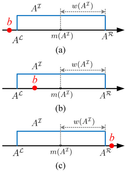
Figure 2. Relation between an interval and a real number. (a) $A^{\mathcal{L}}\ge b$; (b) $A^{\mathcal{L}}\le b\le A^{\mathcal{R}}$; (c) $A^{\mathcal{R}}\le b$.

Equivalently,

$$P\{A^{\mathcal{I}}\le b\}=\left\{\begin{array}{c}0\mathrm{for}m(A^{\mathcal{I}})-w(A^{\mathcal{I}})>b,\hfill \\ \frac{b-m(A^{\mathcal{I}})+w(A^{\mathcal{I}})}{2w(A^{\mathcal{I}})}\mathrm{for}m(A^{\mathcal{I}})-w(A^{\mathcal{I}})\le b\hfill \\ \le m(A^{\mathcal{I}})+w(A^{\mathcal{I}}),\hfill \\ 1\mathrm{for}m(A^{\mathcal{I}})+w(A^{\mathcal{I}})<b.\hfill \end{array}\right.$$

(41)

According to the arithmetic operations between intervals, we have $P\{A^{\mathcal{I}}\ge b\}=P\{-A^{\mathcal{I}}\le -b\}=P\{{A^{\prime }}^{\mathcal{I}}\le b^{\prime }\}$, where ${A^{\prime }}^{\mathcal{I}}=-A^{\mathcal{I}}$ and $b^{\prime }=-b$. Therefore, the possibility degree definition for $P\{A^{\mathcal{I}}\ge b\}$ is omitted for simplicity.

Assuming that a threshold $\xi \in [0,1]$ is given for the possibility degree of the interval constraint $A^{\mathcal{I}}\le b$ based on a decision-maker’s risk tolerance, we obtain $P\{A^{\mathcal{I}}\le b\}\ge \xi$. Therefore, according to the possibility degree definition in (41), the interval constraint $A^{\mathcal{I}}\le b$ with the given ξ can be converted into a deterministic inequality, i.e.,

$$m(A^{\mathcal{I}})+(2\xi -1)w(A^{\mathcal{I}})\le b$$

(42)

The prescribed ξ represents the degree to which a decision-maker tolerates the risk on interval uncertainties. Based on the possibility degree definition of the interval constraint $A^{\mathcal{I}}\le b$, it can be concluded that the bigger ξ we prescribe, the more pessimistic decision we make. In particular, the possibility degree $\xi =0$ (namely $P\{A^{\mathcal{I}}\le b\}\ge 0$) means an absolutely optimistic decision, while $\xi =1$ (namely $P\{A^{\mathcal{I}}\le b\}\ge 1$) means an absolutely pessimistic decision.

3.1.3. Interval Constraint Transformation

After prescribing a threshold of the possibility degree for an interval constraint, we can transform the interval constraint into a deterministic constraint.

Assuming the possibility degree ${\xi }_{\mathrm{eq}}$ is given for the interval equality constraints (12) and (13), we can convert (12) and (13) into deterministic constraints, i.e.,

$$\begin{array}{c}m(P_i(t))+(2{\xi }_{\mathrm{eq}}-1)w(P_i(t))\le V_i(t){\displaystyle \sum _{j=1}^N}{V}_j(t)\left[G_{ij}cos{\theta }_{ij}(t)+B_{ij}sin{\theta }_{ij}(t)\right]\hfill \\ m(P_i(t))+(2{\xi }_{\mathrm{eq}}-1)w(P_i(t))\ge V_i(t){\displaystyle \sum _{j=1}^N}{V}_j(t)\left[G_{ij}cos{\theta }_{ij}(t)+B_{ij}sin{\theta }_{ij}(t)\right]\hfill \end{array}$$

(43)

$$\begin{array}{c}m(Q_i(t))+(2{\xi }_{\mathrm{eq}}-1)w(Q_i(t))\le V_i(t){\displaystyle \sum _{j=1}^N}{V}_j(t)\left[G_{ij}sin{\theta }_{ij}(t)-B_{ij}cos{\theta }_{ij}(t)\right]\hfill \\ m(Q_i(t))+(2{\xi }_{\mathrm{eq}}-1)w(Q_i(t))\ge V_i(t){\displaystyle \sum _{j=1}^N}{V}_j(t)\left[G_{ij}sin{\theta }_{ij}(t)-B_{ij}cos{\theta }_{ij}(t)\right]\hfill \end{array}$$

(44)

where:

$$\begin{array}{c}m(P_i(t))=P_{\mathrm{esu},i}(t)+P_{\mathrm{ev},i}(t)+P_{\mathrm{pcc},i}(t)+m(P_{\mathrm{gt},i}^{\mathcal{I}}(t))+m(P_{\mathrm{wt},i}^{\mathcal{I}}(t))+m(P_{\mathrm{pv},i}^{\mathcal{I}}(t))-m(P_{\mathrm{load},i}^{\mathcal{I}}(t))\hfill \\ w(P_i(t))=w(P_{\mathrm{gt},i}^{\mathcal{I}}(t))+w(P_{\mathrm{wt},i}^{\mathcal{I}}(t))+w(P_{\mathrm{pv},i}^{\mathcal{I}}(t))+w(P_{\mathrm{load},i}^{\mathcal{I}}(t))\hfill \end{array}$$

(45)

$$\begin{array}{c}m(Q_i(t))=Q_{\mathrm{esu},i}(t)+Q_{\mathrm{ev},i}(t)+Q_{\mathrm{pcc},i}(t)+Q_{\mathrm{pv},i}(t)+Q_{\mathrm{wt},i}(t)+m(Q_{\mathrm{gt},i}^{\mathcal{I}}(t))-m(Q_{\mathrm{load},i}^{\mathcal{I}}(t))\hfill \\ w(Q_i(t))=w(Q_{\mathrm{gt},i}^{\mathcal{I}}(t))+w(Q_{\mathrm{load},i}^{\mathcal{I}}(t))\hfill \end{array}$$

(46)

Similarly, the interval inequality constraints (17) with a given possibility degree ${\xi }_{\mathrm{ineq}}$ can be converted into deterministic constraints, i.e.,

$$\begin{array}{c}m(P_{\mathrm{gt},g}^{\mathcal{I}}(t))+(2{\xi }_{\mathrm{ineq}}-1)w(P_{\mathrm{gt},g}^{\mathcal{I}}(t))\le P_{\mathrm{gt},g}^{max}(t)\hfill \\ m(P_{\mathrm{gt},g}^{\mathcal{I}}(t))-(2{\xi }_{\mathrm{ineq}}-1)w(P_{\mathrm{gt},g}^{\mathcal{I}}(t))\ge P_{\mathrm{gt},g}^{min}(t)\hfill \end{array}$$

(47)

$$\begin{array}{c}m(Q_{\mathrm{gt},g}^{\mathcal{I}}(t))+(2{\xi }_{\mathrm{ineq}}-1)w(Q_{\mathrm{gt},g}^{\mathcal{I}}(t))\le Q_{\mathrm{gt},g}^{max}(t)\hfill \\ m(Q_{\mathrm{gt},g}^{\mathcal{I}}(t))-(2{\xi }_{\mathrm{ineq}}-1)w(Q_{\mathrm{gt},g}^{\mathcal{I}}(t))\ge Q_{\mathrm{gt},g}^{min}(t)\hfill \end{array}$$

(48)

3.1.4. Objective Function Transformation

Since the objective function of the obtained scheduling model includes the interval variables $P_{\mathrm{load}}^{\mathcal{I}}(t)$, $P_{\mathrm{wt}}^{\mathcal{I}}(t)$, $P_{\mathrm{pv}}^{\mathcal{I}}(t)$ and $P_{\mathrm{gt}}^{\mathcal{I}}(t)$, the value of the objective function is an interval, namely $F^{\mathcal{I}}=⟨m(F^{\mathcal{I}})w(F^{\mathcal{I}})⟩$, where $m(F^{\mathcal{I}})$ and $w(F^{\mathcal{I}})$ represent the midpoint and width of the objective function, respectively. As far as the problem on maximizing profits is concerned, a decision-maker tends to achieve the maximum midpoint for high profits and the minimum width for low uncertainty. Thus, the objective function (3) can be represented by a multi-objective function, i.e.,

$$max\{m(F^{\mathcal{I}}),-w(F^{\mathcal{I}})\}$$

(49)

where:

$$\begin{array}{c}m(F^{\mathcal{I}})={\displaystyle \sum _{t=1}^T}\left[m(F_{\mathrm{E}}^{\mathcal{I}})-m(F_{\mathrm{C}}^{\mathcal{I}})\right]\hfill \\ w(F^{\mathcal{I}})={\displaystyle \sum _{t=1}^T}\left[w(F_{\mathrm{E}}^{\mathcal{I}})+w(F_{\mathrm{C}}^{\mathcal{I}})\right]\hfill \end{array}$$

(50)

For simplicity, this paper uses a linear weighting method to convert the multi-objective function (49) into a single-objective function, i.e.,

$$maxf=m(F^{\mathcal{I}})-{\xi }_{\mathrm{fun}}w(F^{\mathcal{I}})$$

(51)

where ${\xi }_{\mathrm{fun}}\in [0,1]$ denotes the weighting coefficient. Obviously, the smaller weighting coefficient ${\xi }_{\mathrm{fun}}$ implies that the decision-maker cares more about the midpoint and less about the width. In other words, the decision-maker is willing to obtain more profits at the cost of higher uncertain risks.

3.2. Transformation for Absolute-Value Function

To reduce the computational expense, we need to make a transformation for the ABS function. In mathematics, for an arbitrary real number $Y\in \mathbb{R}$, its ABS function $\left|Y\right|$ can be expressed to be $\left|Y\right|=W+Z$, where W and Z are called the slack variables, which should be meet the following complementary conditions [38]:

$$\begin{array}{c}Y=W-Z,WZ=0,W\ge 0,Z\ge 0\hfill \end{array}$$

(52)

According to the above mathematical transformation, the equality (6) can be transformed into:

$$\begin{array}{c}{P}_{\mathrm{pcc}}^{\mathrm{s}}(t)=Z_{\mathrm{pcc}}\hfill \\ P_{\mathrm{pcc}}^{\mathrm{b}}(t)=W_{\mathrm{pcc}}\hfill \\ P_{\mathrm{pcc}}=W_{\mathrm{pcc}}-Z_{\mathrm{pcc}}\hfill \\ W_{\mathrm{pcc}}{Z}_{\mathrm{pcc}}=0\hfill \\ W_{\mathrm{pcc}}\ge 0,Z_{\mathrm{pcc}}\ge 0\hfill \end{array}$$

(53)

where $W_{\mathrm{pcc}}$ and $Z_{\mathrm{pcc}}$ are slack variables; $P_{\mathrm{pcc}}=W_{\mathrm{pcc}}-Z_{\mathrm{pcc}}$, $W_{\mathrm{pcc}}{Z}_{\mathrm{pcc}}=0$, $W_{\mathrm{pcc}}\ge 0$ and $Z_{\mathrm{pcc}}\ge 0$ are complementary conditions.

Similarly, the equality (10) can be transformed into:

$$\begin{array}{c}{F}_{\mathrm{C},\mathrm{esu}}(t)={\displaystyle \sum _{s=1}^{\mathcal{S}}}{\gamma }_{\mathrm{esu},s}\left[W_{\mathrm{esu},s}(t)+Z_{\mathrm{esu},s}(t)\right]\hfill \\ P_{\mathrm{esu},s}=W_{\mathrm{esu},s}(t)-Z_{\mathrm{esu},s}(t)\hfill \\ W_{\mathrm{esu},s}(t)Z_{\mathrm{esu},s}(t)=0\hfill \\ W_{\mathrm{esu},s}(t)\ge 0,Z_{\mathrm{esu},s}(t)\ge 0\hfill \end{array}$$

(54)

where $W_{\mathrm{esu},s}(t)$ and $Z_{\mathrm{esu},s}(t)$ are slack variables; $P_{\mathrm{esu},s}=W_{\mathrm{esu},s}(t)-Z_{\mathrm{esu},s}(t)$, $W_{\mathrm{esu},s}{Z}_{\mathrm{esu},s}=0$, $W_{\mathrm{esu},s}\ge 0$ and $Z_{\mathrm{esu},s}\ge 0$ are complementary conditions.

The equality (11) can be transformed into:

$$\begin{array}{c}{F}_{\mathrm{C},\mathrm{ev}}(t)={\displaystyle \sum _{v=1}^{\mathcal{V}}}{\gamma }_{\mathrm{ev},v}\left[W_{\mathrm{ev},v}(t)+Z_{\mathrm{ev},v}(t)\right]\hfill \\ P_{\mathrm{ev},v}(t)=W_{\mathrm{ev},v}(t)-Z_{\mathrm{ev},v}(t)\hfill \\ W_{\mathrm{ev},v}(t)Z_{\mathrm{ev},v}(t)=0\hfill \\ W_{\mathrm{ev},v}(t)\ge 0,Z_{\mathrm{ev},v}(t)\ge 0\hfill \end{array}$$

(55)

where $W_{\mathrm{ev},v}(t)$ and $Z_{\mathrm{ev},v}(t)$ are slack variables; $P_{\mathrm{ev},v}(t)=W_{\mathrm{ev},v}(t)-Z_{\mathrm{ev},v}(t)$, $W_{\mathrm{ev},v}{Z}_{\mathrm{ev},v}=0$, $W_{\mathrm{ev},v}\ge 0$ and $Z_{\mathrm{ev},v}\ge 0$ are complementary conditions.

After the above transformations, the scheduling model of the microgrid has been converted into a general nonlinear programming model without the interval constraints and the ABS functions. In the following numerical simulations, considering that the optimization model is nonlinear and nonconvex, this paper uses the professional optimization software (GAMS) to solve the model.

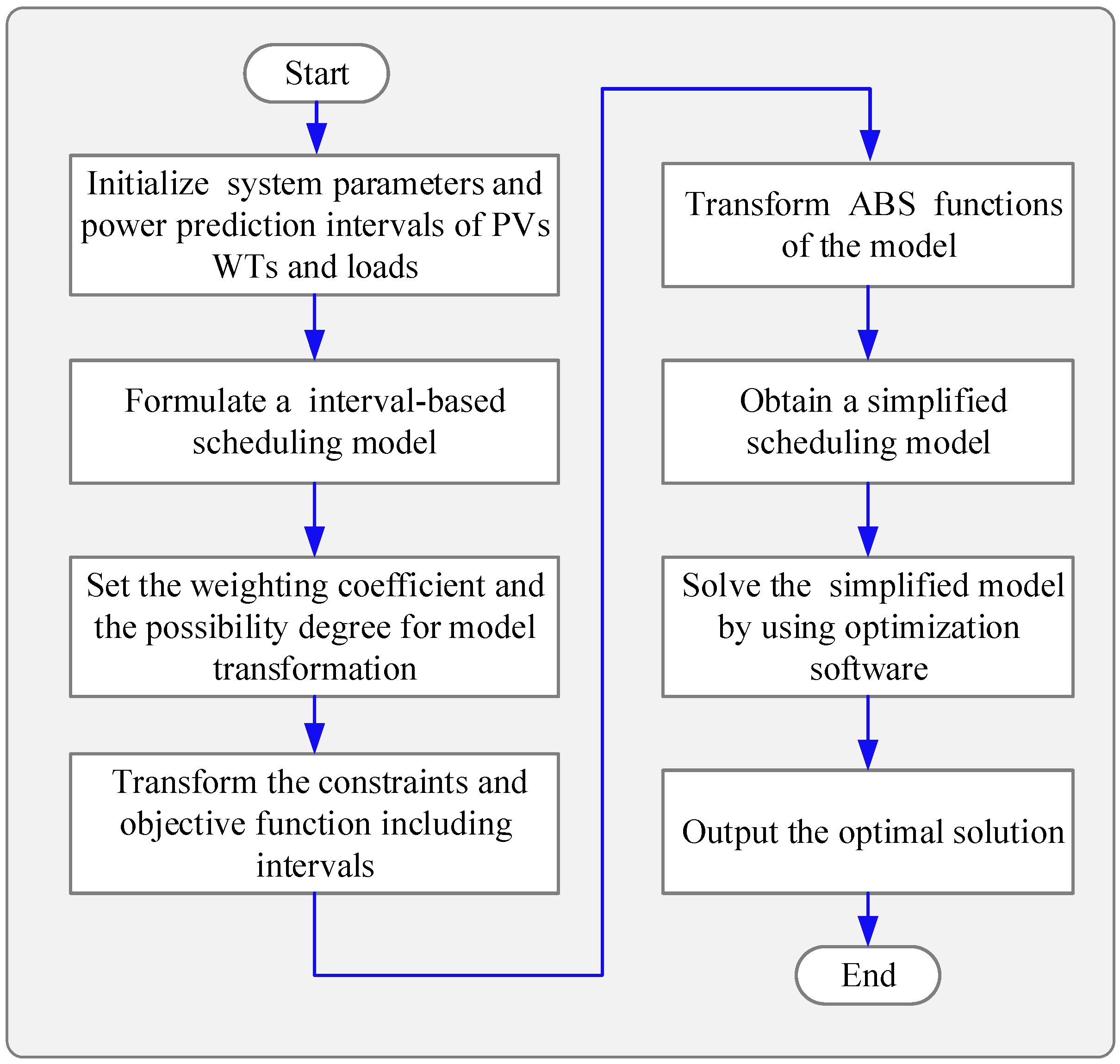
The details about the application for the proposed interval-based optimization model of the microgrid are summarized in Figure 3.

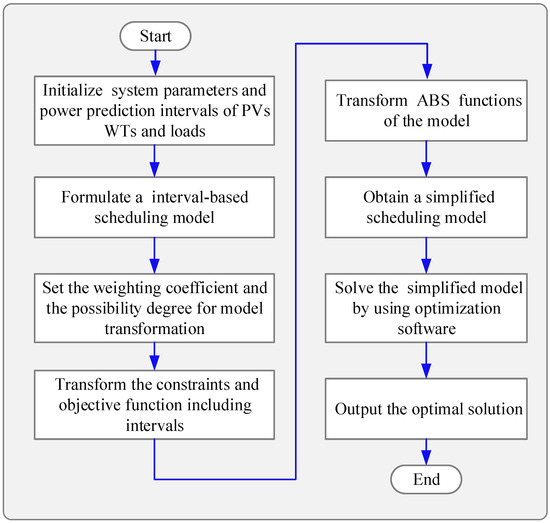
Figure 3. Flow chart for solving the interval-based optimization model.

3.3. A Simple Example for Model Transformation

For readers to understand the above model transformation well, we take a simple example for illustration. An optimization problem is given as follows:

$$\begin{array}{c}\hfill maxF=3X_1^2+2X_2^2+Y^{\mathcal{I}}{X}_2\end{array}$$

(56a)

$$\begin{array}{c}\hfill \mathrm{s}.\mathrm{t}.{\mathrm{X}}_1^3+{\mathrm{X}}_2^2+{\mathrm{Y}}^{\mathcal{I}}=0\end{array}$$

(56b)

$$\begin{array}{c}\hfill X_1+X_2+Y^{\mathcal{I}}\le 3\end{array}$$

(56c)

$$\begin{array}{c}\hfill |X_1|+X_2^2-X_2\le 4\end{array}$$

(56d)

$$\begin{array}{c}\hfill -5\le X_1\le 5,0\le X_2\end{array}$$

(56e)

where $X_1$ and $X_2$ are the decision variables; $Y^{\mathcal{I}}=[1.2,1.8]=\{y:1.2\le y\le 1.8\}$ denotes the interval of uncertain variable y. The midpoint and width of $Y^{\mathcal{I}}$ are $m(Y^{\mathcal{I}})=(1.2+1.8)/2=1.5$ and $w(Y^{\mathcal{I}})=1.8-1.2=0.6$, respectively.

The interval equality (56b) can be converted into two interval inequalities equivalently, i.e.,

$$\begin{array}{c}{X}_1^3+X_2^2+Y^{\mathcal{I}}\le 0\hfill \\ X_1^3+X_2^2+Y^{\mathcal{I}}\ge 0\hfill \end{array}$$

(57)

By choosing ${\xi }_{\mathrm{eq}}$ as the possibility degree of (57), we can convert (57) into two deterministic constraints according to (42), i.e.,

$$\begin{array}{c}m(X_1^3+X_2^2+Y^{\mathcal{I}})+(2{\xi }_{\mathrm{eq}}-1)w(X_1^3+X_2^2+Y^{\mathcal{I}})\le 0\hfill \\ m(X_1^3+X_2^2+Y^{\mathcal{I}})+(2{\xi }_{\mathrm{eq}}-1)w(X_1^3+X_2^2+Y^{\mathcal{I}})\ge 0\hfill \end{array}$$

(58)

namely,

$$\begin{array}{c}{X}_1^3+X_2^2+m(Y^{\mathcal{I}})+(2{\xi }_{\mathrm{eq}}-1)w(Y^{\mathcal{I}})\le 0\hfill \\ X_1^3+X_2^2+m(Y^{\mathcal{I}})+(2{\xi }_{\mathrm{eq}}-1)w(Y^{\mathcal{I}})\ge 0\hfill \end{array}$$

(59)

By substituting $m(Y^{\mathcal{I}})=1.5$ and $w(Y^{\mathcal{I}})=0.6$ into (59), it yields:

$$\begin{array}{c}{X}_1^3+X_2^2+1.5+0.6(2{\xi }_{\mathrm{eq}}-1)\le 0\hfill \\ X_1^3+X_2^2+1.5+0.6(2{\xi }_{\mathrm{eq}}-1)\ge 0\hfill \end{array}$$

(60)

namely,

$$X_1^3+X_2^2+1.5+0.6(2{\xi }_{\mathrm{eq}}-1)=0$$

(61)

Similarly, the interval inequality (56c) can be transformed into a deterministic constraint by using (42), i.e.,

$$X_1+X_2+1.5+0.6(2{\xi }_{\mathrm{ineq}}-1)\le 3$$

(62)

where ${\xi }_{\mathrm{ineq}}$ is the given possibility degree of the interval inequality (56c).

According to the mathematical transformation (52) for the ABS function, the constraint (56d) can be converted into the following constraints, i.e.,

$$\begin{array}{c}W+Z+X_2^2-X_2\le 4\hfill \\ X_1=W-Z\hfill \\ WZ=0,W\ge 0,Z\ge 0\hfill \end{array}$$

(63)

where W and Z are the slack variables; $WZ=0$, $W\ge 0$ and $Z\ge 0$ are the complementary conditions.

Assuming that ${\xi }_{\mathrm{fun}}$ is the weighting coefficient of the interval objective function (56a), we transform (56a) into a deterministic objective function by using (51), i.e.,

$$maxf=m(F^{\mathcal{I}})-{\xi }_{\mathrm{fun}}w(F^{\mathcal{I}})$$

(64)

namely,

$$maxf=3X_1^2+2X_2^2+1.5X_2-0.6{\xi }_{\mathrm{fun}}{X}_2$$

(65)

Through the above transformations, the optimization problem (56) has been converted into a general optimization model without intervals and the ABS function, i.e.,

$$\begin{array}{c}\hfill maxf=3X_1^2+2X_2^2+1.5X_2-0.6{\xi }_{\mathrm{fun}}{X}_2\\ \hfill \mathrm{s}.\mathrm{t}.X_1^3+X_2^2+1.5+0.6(2{\xi }_{\mathrm{eq}}-1)=0\\ \hfill X_1+X_2+1.5+0.6(2{\xi }_{\mathrm{ineq}}-1)\le 3\\ \hfill W+Z+X_2^2-X_2\le 4\\ \hfill X_1=W-Z\\ \hfill WZ=0,W\ge 0,Z\ge 0\\ \hfill -5\le X_1\le 5,0\le X_2\end{array}$$

(66)

where ${\xi }_{\mathrm{fun}}$, ${\xi }_{\mathrm{eq}}$ and ${\xi }_{\mathrm{ineq}}$ are the preassigned parameters.

For the optimization model (66), we can use the existing nonlinear programming algorithms or the professional optimization software to calculate the optimal solution. Here, the calculation process is omitted for brevity.

4. Case Studies

In this section, a microgrid test system, which is modified from the benchmark LVnetwork in the EU project “Microgrid” [45], is used to test the proposed scheduling method. The single-line diagram of the microgrid test system is shown in Figure 4.

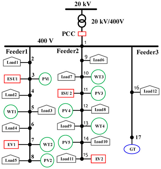
Figure 4. Single-line diagram of the microgrid test system.

In the test system, the impedance parameters of the network lines (120 mm${}^2$ Al XLPEtwisted cable) are given as: $R=0.284\mathsf{\Omega }/\mathrm{km}$, $X=0.083\mathsf{\Omega }/\mathrm{km}$ and pole-to-pole distance $L=35\mathrm{m}$.

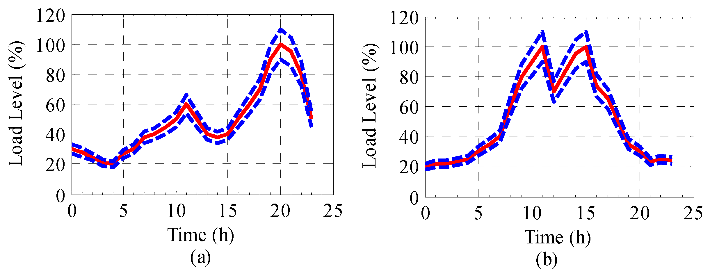
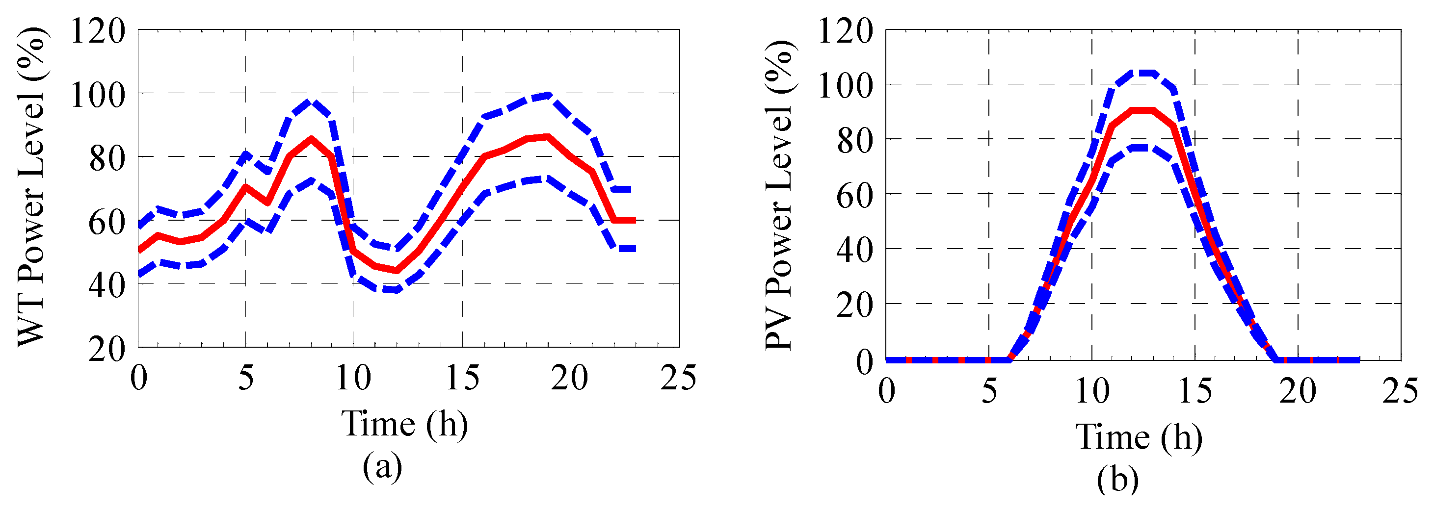
The loads on Feeder 1 represent residential power consumption, while the loads on Feeders 2 and 3 represent industrial power consumption. The rated apparent power ($S_{\mathrm{rate}}$) and power factor ($cos\psi$) of the loads are listed in Table 1, and the prediction intervals of loads in 24 h are shown in Figure 5. The load prediction error is assumed to be $\pm 10\%$ of the prediction value (midpoint). The parameters of PVs and WTs are given in Table 2, and the power prediction intervals in 24 h are shown in Figure 6. The power prediction error of PVs and WTs is assumed to be $\pm 15\%$ of the prediction value (midpoint). The parameters of ESUs, EVs and GT are given in Table 3.

Table 1. Parameters of loads of the microgrid.

Name	Node	${\mathit{S}}_{\mathbf{rate}}$ (kVA)	PF ($cos\mathit{\psi }$)
Load 1	2	40	0.85
Load 2	4	40	0.85
Load 3	5	40	0.85
Load 4	6	40	0.85
Load 5	8	40	0.85
Load 6	9	50	0.90
Load 7	10	50	0.90
Load 8	12	50	0.90
Load 9	13	50	0.90
Load 10	14	50	0.90
Load 11	15	50	0.90
Load 12	16	200	0.95

Figure 5. Prediction intervals of loads in 24 h (the dotted lines denote the upper and lower bounds, and the real lines denote predicted value). (a) Loads on Feeder 1; (b) loads on Feeders 2 and 3.

Table 2. Parameters of PVs and WTs of the microgrid.

Name	Node	${\mathit{P}}_{\mathbf{rate}}$ (kW)	${\mathit{Q}}^{min}$ (kvar)	${\mathit{Q}}^{max}$ (kvar)
PV1	3	20	−8.0	8.0
PV2	8	20	−8.0	8.0
PV3	11	20	−8.0	8.0
PV4	12	30	−10.0	10.0
PV5	14	30	−10.0	10.0
WT1	5	25	−5.0	5.0
WT2	7	25	−5.0	5.0
WT3	10	25	−5.0	5.0
WT4	13	25	−5.0	5.0

Figure 6. Power prediction intervals of PVs and WTs in 24 h (the dotted lines denote the upper and lower bounds, and the real lines denote predicted value). (a) Active power of WTs; (b) active power of PVs.

Table 3. Parameters of energy storage units (ESUs), EVs and gas turbine (GT) of the microgrid.

Name	Node	γ (CNY/kWh)	${\mathit{P}}^{min}$ (kW)	${\mathit{P}}^{max}$ (kW)	${\mathit{Q}}^{min}$ (kvar)	${\mathit{Q}}^{max}$ (kvar)	${\mathit{E}}^{min}$ (kWh)	${\mathit{E}}^{max}$ (kWh)	$\mathit{E}(0)$ (kWh)
ESU1	3	0.20	−100	100	−20	20	60	600	90
ESU2	11	0.20	−100	100	−20	20	60	600	90
EV1	7	0.25	−75	75	−10	10	40	400	60
EV2	15	0.25	−75	75	−10	10	40	400	60
GT	17	0.65	0.0	80	−15	15	–	–	–

The day-ahead price information from the electricity market is given in Table 4. In the tests, it is assumed that the traveling time of EVs is two hours (8:00–9:00 and 17:00–18:00), the average traveling power of EVs is $100\mathrm{kW}$, and the required minimum energy for EV traveling is $150\mathrm{kWh}$. Thus, the corresponding parameters of each EV for the simulations are set as: $t_{\mathrm{mor},\mathrm{dep}}=8$, $t_{\mathrm{mor},\mathrm{ret}}=9$, $t_{\mathrm{aft},\mathrm{dep}}=17$, $t_{\mathrm{aft},\mathrm{ret}}=18$, $k=1$, $P_{\mathrm{ev}}^{\mathrm{av}}=100$ and $E_{\mathrm{ev},\mathrm{dep}}^{min}=150$.

Table 4. Time-of-use price in a day.

Periods	${\mathit{\gamma }}_{\mathbf{b}}$ (CNY/kWh)	${\mathit{\gamma }}_{\mathbf{s}}$ (CNY/kWh)	${\mathit{\gamma }}_{\mathbf{sub}}$ (CNY/kWh)
00:00–08:00	0.39	0.30	0.42
08:00–12:00	1.65	0.95	0.42
12:00–17:00	0.87	0.56	0.42
17:00–21:00	1.65	0.95	0.42
21:00–24:00	0.87	0.56	0.42

For guaranteeing the voltage quality, the allowed deviation of all of the bus voltage is limited to $\pm 5\%$ of the rated value.

The scheduling strategy is affected by the weighting coefficient (${\xi }_{\mathrm{fun}}$) of the objective function, the possibility degree (${\xi }_{\mathrm{eq}}$) of the interval equality constraints (13) and the possibility degree (${\xi }_{\mathrm{ineq}}$) of the interval inequality constraints (17). In order to reduce the difficulty in analysis, the possibility degree of the interval inequality constraints is fixed to ${\xi }_{\mathrm{ineq}}\equiv 1$, which means that the scheduling strategy completely satisfies the interval inequality constraints. In other words, the decision-maker is absolutely pessimistic about the interval inequality constraints (17).

The numerical simulations are performed with different values of ${\xi }_{\mathrm{fun}}$ and ${\xi }_{\mathrm{eq}}$, and the corresponding profit intervals of the microgrid are listed in Table 5. From the results, we can see that with the same weighting coefficient (${\xi }_{\mathrm{fun}}$), as the possibility degree (${\xi }_{\mathrm{eq}}$) increases, the midpoint, the width and the expected value of the profit interval increase. The bigger possibility degree (${\xi }_{\mathrm{eq}}$) means that the decision-maker expects the more power output of renewable resources and the higher load level to increase the profits, at the cost of the bigger risk on the prediction uncertainties. If the decision-maker fixes a small possibility degree (${\xi }_{\mathrm{eq}}$), as the weighting coefficient (${\xi }_{\mathrm{fun}}$) increases, the midpoint and the width of the profit interval barely change, but the expected profit decreases since the objective function (45) is inversely proportional to the weighting coefficient (${\xi }_{\mathrm{fun}}$).

Table 5. Profit intervals of the microgrid.

${\mathit{\xi }}_{\mathbf{fun}}$	${\mathit{\xi }}_{\mathbf{eq}}$	Midpoint (CNY)	Width (CNY)	Expected Profit (CNY)
0.0	0.0	7142.81	1055.36	7142.81
0.0	0.5	7144.19	1087.78	7144.19
0.0	1.0	7702.77	1676.16	7702.77
0.5	0.0	7142.81	1055.36	6615.13
0.5	0.5	7144.19	1055.36	6616.51
0.5	1.0	7701.70	1669.45	6866.98
1.0	0.0	7142.81	1055.36	6087.45
1.0	0.5	7144.19	1055.36	6088.83
1.0	1.0	7401.33	1309.42	6091.91

Table 6 lists the iterations and the computation time for solving the optimization model. From the comparative results, we can see that the computation time is reduced significantly after the ABS functions are removed.

Table 6. Computation time for solving the optimization model.

Optimization Model	Iterations	Time (s)
Remove ABS Function	438	1.22
Include ABS Function	2826	13.76

Due to page limitations, we choose one of the simulation cases (${\xi }_{\mathrm{eq}}=0.5$, ${\xi }_{\mathrm{fun}}=0.5$) for analysis. The simulation results are shown in Figure 7, Figure 8, Figure 9, Figure 10, Figure 11 and Figure 12.

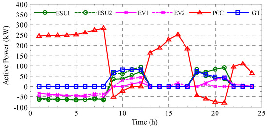
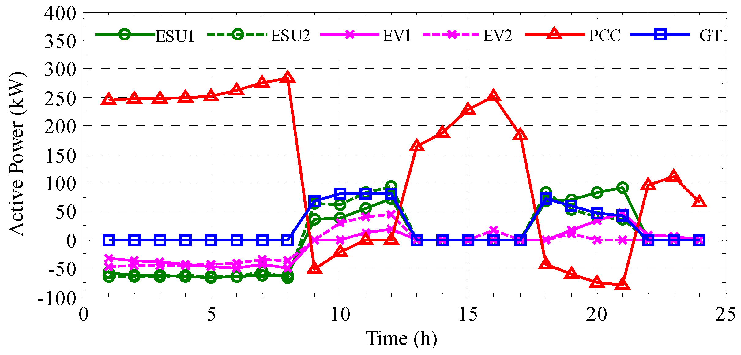
Figure 7. Active power of ESUs, EVs, point of common coupling (PCC) and GT in 24 h.

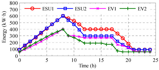
Figure 8. Energy of ESUs and EVs in 24 h.

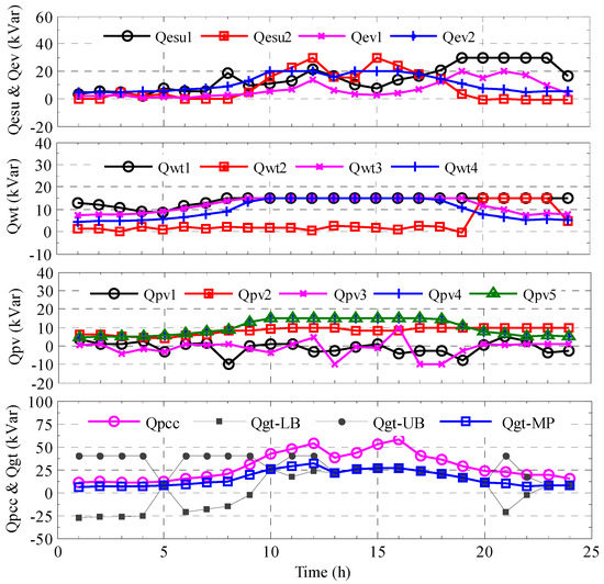
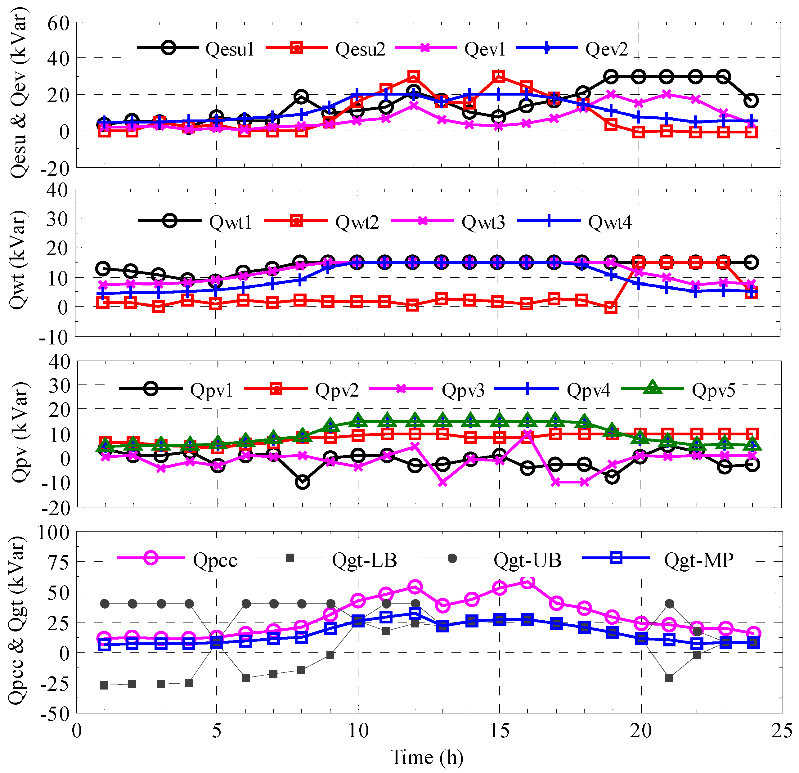
Figure 9. Reactive power of ESUs, EVs, WTs, PVs, PCC and GT in 24 h.

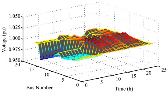
Figure 10. Voltage amplitude of the microgrid in 24 h.

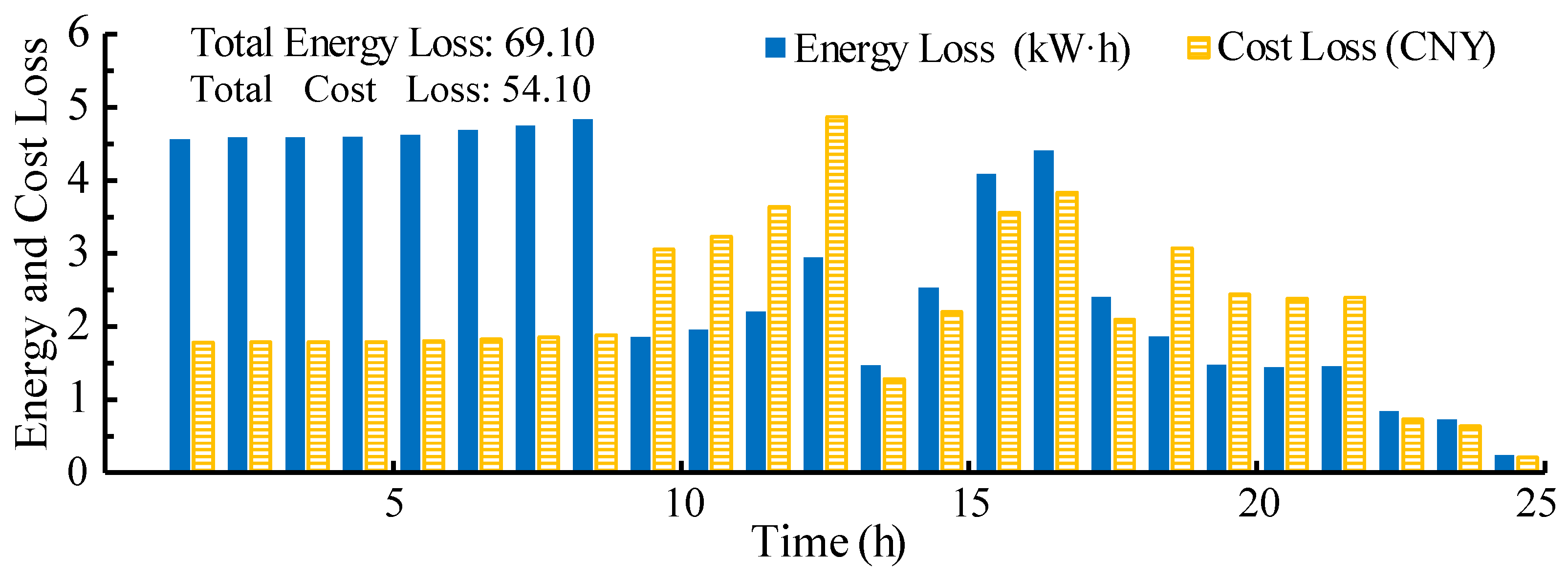
Figure 11. Energy and cost loss of the microgrid in 24 h.

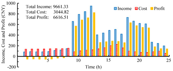
Figure 12. Income, cost and profits of the microgrid in 24 h.

Figure 7 shows the scheduling strategy for the active power of all of the controllable resources. From the results, we can see that the ESUs and the EVs are charged in a low-price time and discharged in a high-price time. In this way, the ESUs and the EVs generate profits by taking advantage of the time-of-use price. It is worthy to note that the active power of the EVs is zero at 08:00 and 17:00 since the EVs are not at the charging station. Seeing the active power curve of PCC, we can find that the microgrid purchases the electricity from the main grid in low-price or mid-price periods ($P_{\mathrm{pcc}}>0$) and sells the electricity to the main grid in high-price periods ($P_{\mathrm{pcc}}<0$). The GT outputs active power in the high-price periods (08:00–12:00 and 17:00–21:00) because only in these periods, the electric price is higher than the cost. Here, it should be noted that the active power $P_{\mathrm{gt}}^{\mathcal{I}}$ of GT degenerates into a real number to reduce the uncertainty of the profits, though $P_{\mathrm{gt}}^{\mathcal{I}}$ is originally designed to be an interval decision variable.

The residual energy curves of ESUs and EVs in 24 h are shown in Figure 8. The initial energies of ESUs and EVs are 90 kWh and 60 kWh, respectively. At 08:00, ESUs and EVs are fully charged; in the high-price periods, ESUs and EVs feed their power to the grid; at the end of a day, the residual energies of ESUs and EVs drop to the initial values, which means that the energies in ESUs and EVs are kept balanced in a whole day.

Figure 9 shows the reactive power of ESUs, EVs, WTs, PVs, PCC and GT in 24 h. The reactive power outputs of the controllable resources are adjusted in different periods to keep all of the bus voltages in the allowed range and reduce the active power loss of microgrid. It can be found from the results that PV1 and PV3 absorb excess reactive power on Bus 3 and Bus 11, while the rest of the resources provide the reactive power for the microgrid. Here, it should be noted that the reactive power of PVs is nonzero in the periods without sunlight (before 6:00 a.m. and after 19:00 p.m. in a day), though the active power of PVs is zero; see Figure 6b. The reason is that in these periods, the PV converter serves as a static var generator (SVG) whose reactive power output does not depend on sunlight. Therefore, the PV converter can generate reactive power in 24 h. As mentioned earlier, the reactive power $Q_{\mathrm{gt}}^{\mathcal{I}}$ of GT is designed to be an interval decision variable for coping with the reactive power uncertainties of loads. The lower bound, the upper bound and the midpoint of $Q_{\mathrm{gt}}^{\mathcal{I}}$ are shown in the fourth subfigure of Figure 9. It can be seen that the width of $Q_{\mathrm{gt}}^{\mathcal{I}}$ varies in different periods, and the widest interval reaches [−26, 28] kvar.

The bus voltages in 24 h are shown in Figure 10. It can be seen that all of the bus voltages stay in the prescribed range, which means that the optimal scheduling scheme can guarantee the voltage quality of the microgrid.

The energy loss and the cost loss of the whole microgrid are illustrated in Figure 11. From the results, we can find that the energy loss in 0:00–8:00 is higher than that in other periods. The reason is that in 0:00–8:00, the amount of power flows from the main grid into the microgrid through distribution lines to feed ESUs, EVs and loads, and thus, the energy loss on the distribution lines is relatively high. By contrast, in other periods, the transmission loss is reduced greatly, since much power demand is balanced locally. From the cost loss statistics, it can be seen that the cost loss in the high-price periods is high, because the cost loss is equal to the product of the energy loss and the electric price.

Figure 12 shows the income, the cost and the profits of the microgrid. It is illustrated that the profits are gained in the high-price and mid-price periods. In these periods, the profits consist of the electricity sales of ESUs, EVs, WTs, PVs, as well as the government’s subsidies to the renewable energy. It should be noted that the profits in 0:00–08:00 are negative, since a large amount of power is purchased from the main grid to charge ESUs and EVs in this period.

5. Conclusions

This paper studies the optimal scheduling problem of a grid-connected microgrid with ESUs, EVs, PVs, WTs and GTs. The intervals are used to describe the uncertainties of the renewable resources and the loads in the microgrid, since it is easier to know the bounds of the uncertain variables than to obtain their probability distribution functions. To reduce the complexity caused by the interval variables, the possibility degree comparison between an interval and a real number is adopted to remove the interval variables in the optimization model. In addition, some slack variables and complementary conditions are introduced to eliminate the ABS functions to save the computational cost. The simulation results show that the proposed method can find the interval of profits and obtain the optimal expected profits, as long as the decision-maker assigns the values for the weighting coefficient of the objective function and the possibility degrees of the interval constraints. It should be pointed out that how to reasonably choose the aforementioned values for the interval optimization problem will be studied in further research.

References

- Basak, P.; Chowdhury, S.; Dey, S.H.N.; Chowdhury, S.P. A literature review on integration of distributed energy resources in the perspective of control, protection and stability of microgrid. Renew. Sustain. Energy Rev. 2012, 16, 5545–5556. [Google Scholar] [CrossRef]
- Mehrizi-Sani, A.; Iravani, R. Potential-function based control of a microgrid in islanded and grid-connected modes. IEEE Trans. Power Syst. 2010, 25, 1883–1891. [Google Scholar] [CrossRef]
- Lv, T.; Ai, Q.; Zhao, Y. A bi-level multi-objective optimal operation of grid-connected microgrids. Electr. Power Syst. Res. 2016, 131, 60–70. [Google Scholar] [CrossRef]
- Mahmoud, M.S.; Saif, U.M.; Sunni, F.M.A.L. Review of microgrid architectures—A system of systems perspective. IET Renew. Power Gener. 2015, 9, 1064–1078. [Google Scholar] [CrossRef]
- Jimeno, J.; Anduaga, J.; Oyarzabal, J.; De Muro, A.G. Architecture of a microgrid energy management system. Eur. Trans. Electr. Power 2011, 21, 1142–1158. [Google Scholar] [CrossRef]
- Chen, C.; Duan, S.; Cai, T.; Liu, B. Smart energy management system for optimal microgrid economic operation. IET Renew. Power Gener. 2011, 5, 258–267. [Google Scholar] [CrossRef]
- Tian, P.; Xiao, X.; Wang, K.; Ding, R. A hierarchical energy management system based on hierarchical optimization for microgrid community economic operation. IEEE Trans. Smart Grid. 2016, 7, 2230–2241. [Google Scholar] [CrossRef]
- Tsikalakis, A.G.; Hatziargyriou, N.D. Centralized control for optimizing microgrids operation. IEEE Trans. Energy Convers. 2008, 23, 241–248. [Google Scholar] [CrossRef]
- Shafiee, Q.; Dragicevic, T.; Vasquez, J.C.; Guerrero, J.M. Hierarchical control for multiple DC-Microgrids clusters. IEEE Trans. Energy Convers. 2014, 29, 922–933. [Google Scholar] [CrossRef]
- Khan, M.R.B.; Jidin, R.; Pasupuleti, J. Multi-agent based distributed control architecture for microgrid energy management and optimization. Energy Convers. Manag. 2016, 112, 288–307. [Google Scholar] [CrossRef]
- Meng, L.; Sanseverino, E.R.; Luna, A.; Dragicevic, T.; Vasquez, J.C.; Guerrero, J.M. Microgrid supervisory controllers and energy management systems: A literature review. Renew. Sustain. Energy Rev. 2016, 60, 1263–1273. [Google Scholar] [CrossRef]
- Wang, R.; Wang, P.; Xiao, G. A robust optimization approach for energy generation scheduling in microgrids. Energy Convers. Manag. 2015, 106, 597–607. [Google Scholar] [CrossRef]
- Khalid, M.; Ahmadi, A.; Savkin, A.V.; Agelidis, V.G. Minimizing the energy cost for microgrids integrated with renewable energy resources and conventional generation using controlled battery energy storage. Renew. Energy 2016, 97, 646–655. [Google Scholar] [CrossRef]
- Conti, S.; Nicolosi, R.; Rizzo, S.A.; Zeineldin, H.H. Optimal dispatching of distributed generators and storage systems for MV islanded microgrids. IEEE Trans. Power Deliv. 2012, 27, 1243–1251. [Google Scholar] [CrossRef]
- Belgana, A.; Rimal, B.P.; Maier, M. Multi-objective pricing game among interconnected smart microgrids. In Proceedings of the PES General Meeting, Conference & Exposition, Washington, DC, USA, 27–31 July 2014; pp. 1–5.
- Nguyen, D.T.; Le, L.B. Optimal bidding strategy for microgrids considering renewable energy and building thermal dynamics. IEEE Trans. Smart Grid 2014, 5, 1608–1620. [Google Scholar] [CrossRef]
- Bahramara, S.; Moghaddam, M.P.; Haghifam, M.R. A bi-level optimization model for operation of distribution networks with micro-grids. Int. J. Electr. Power Energy Syst. 2016, 82, 169–178. [Google Scholar] [CrossRef]
- Alharbi, W.; Raahemifar, K. Probabilistic coordination of microgrid energy resources operation considering uncertainties. Electr. Power Syst. Res. 2015, 128, 1–10. [Google Scholar] [CrossRef]
- Mohammadi, S.; Mozafari, B.; Solymani, S.; Niknam, T. Stochastic scenario-based model and investigating size of energy storage for PEM-fuel cell unit commitment of micro-grid considering profitable strategies. IET Gener. Transm. Distrib. 2014, 8, 1228–1243. [Google Scholar] [CrossRef]
- Talari, S.; Yazdaninejad, M.; Haghifam, M.R. Stochastic-based scheduling of the microgrid operation including wind turbines, photovoltaic cells, energy storage and responsive loads. IET Gener. Transm. Distrib. 2015, 9, 1498–1509. [Google Scholar] [CrossRef]
- Nguyen, T.A.; Crow, M.L. Stochastic optimization of renewable-based microgrid operation incorporating battery operating cost. IEEE Trans. Power Syst. 2016, 31, 2289–2296. [Google Scholar] [CrossRef]
- Kou, P.; Liang, D.; Gao, L.; Gao, F. Stochastic coordination of plug-in electric vehicles and wind turbines in microgrid: A model predictive control approach. IEEE Trans. Smart Grid 2016, 7, 1537–1551. [Google Scholar] [CrossRef]
- Mazidi, M.; Zakariazadeh, A.; Jadid, S.; Siano, P. Integrated scheduling of renewable generation and demand response programs in a microgrid. Energy Convers. Manag. 2014, 86, 1118–1127. [Google Scholar] [CrossRef]
- Momoh, J.A.; Ma, X.W.; Tomsovic, K. Overview and literature survey of fuzzy set theory in power systems. IEEE Trans. Power Syst. 1995, 10, 1676–1690. [Google Scholar] [CrossRef]
- Chaouachi, A.; Kamel, R.M.; Andoulsi, R.; Nagasaka, K. Multiobjective intelligent energy management for a microgrid. IEEE Trans. Ind. Electron. 2013, 60, 1688–1699. [Google Scholar] [CrossRef]
- Farzin, H.; Fotuhi-Firuzabad, M.; Moeini, M. A stochastic multi-objective framework for optimal scheduling of Energy storage systems in Microgrids. IEEE Trans. Smart Grid. 2017, 8, 117–127. [Google Scholar] [CrossRef]
- Mei, S.; Guo, W.; Wang, Y.; Liu, F.; Wei, W. A game model for robust optimization of power systems and its application. Proc. CSEE. 2013, 33, 47–57. [Google Scholar]
- Di Silvestre, M.L.; Graditi, G.; Ippolito, M.G.; Riva Sanseverino, E.; Zizzo, G. Robust multi-objective optimal dispatch of distributed energy resources in micro-grids. In Proceedings of the 2011 IEEE Trondheim PowerTech, Trondheim, Norway, 19–23 June 2011.
- Jiang, R.; Wang, J.; Guan, Y. Robust unit commitment with wind power and pumped storage hydro. IEEE Trans. Power Syst. 2012, 27, 800–810. [Google Scholar] [CrossRef]
- Zhang, Y.; Gatsis, N.; Giannakis, G.B. Robust energy management for microgrids with high-penetration renewables. IEEE Trans. Sustain. Energy 2013, 4, 944–953. [Google Scholar] [CrossRef]
- Liu, K.; Guan, X.; Gao, F.; Zhai, Q.; Wu, J. Self-balancing robust scheduling with flexible batch loads for energy intensive corporate microgrid. Appl. Energy 2015, 159, 391–400. [Google Scholar] [CrossRef]
- Yu, N.; Kang, J.S.; Chang, C.C.; Lee, T.Y.; Lee, D.Y. Robust economic optimization and environmental policy analysis for microgrid planning: An application to Taichung Industrial Park, Taiwan. Energy 2016, 113, 671–682. [Google Scholar] [CrossRef]
- Valencia, F.; Saez, J.C.; Marin, L.G. Robust energy management system for a microgrid based on a fuzzy prediction interval model. IEEE Trans. Smart Grid 2016, 7, 1486–1494. [Google Scholar] [CrossRef]
- Tong, S.C. Interval number and fuzzy number linear programmings. Fuzzy Sets Syst. 1994, 66, 301–306. [Google Scholar]
- Jiang, C.; Han, X.; Liu, G.R.; Liu, G.P. A nonlinear interval number programming method for uncertain optimization problems. Eur. J. Oper. Res. 2008, 188, 1–13. [Google Scholar] [CrossRef]
- Wang, Y.; Xia, Q.; Kang, C. Unit commitment with volatile node injections by using interval optimization. IEEE Trans. Power Syst. 2011, 26, 1705–1713. [Google Scholar] [CrossRef]
- Zhou, M.; Xia, S.; Li, G.; Han, X. Interval optimization combined with point estimate method for stochastic security-constrained unit commitment. Int. J. Electr. Power Energy Syst. 2014, 63, 276–284. [Google Scholar] [CrossRef]
- Ding, T.; Bo, R.; Gu, W.; Guo, Q.; Sun, H. Absolute value constraint based method for interval optimization to SCED model. IEEE Trans. Power Syst. 2014, 29, 980–981. [Google Scholar] [CrossRef]
- Wang, S.; Fan, X.; Han, L.; Ge, L. Improved interval optimization method based on differential evolution for microgrid economic dispatch. Electr. Power Compon. Syst. 2015, 43, 1882–1890. [Google Scholar] [CrossRef]
- Saez, D.; Avila, F.; Olivares, D.; Canizares, C.; Marin, L. Fuzzy prediction interval models for forecasting renewable resources and loads in microgrids. IEEE Trans. Smart Grid 2015, 6, 548–556. [Google Scholar] [CrossRef]
- Gabash, A.; Li, P. Active-reactive optimal power flow in distribution networks with embedded generation and battery storage. IEEE Trans. Power Syst. 2012, 27, 2026–2035. [Google Scholar] [CrossRef]
- Atwa, Y.M.; El-Saadany, E.F. Probabilistic approach for optimal allocation of wind-based distributed generation in distribution systems. IET Renew. Power Gener. 2011, 5, 79–88. [Google Scholar] [CrossRef]
- Moore, R.E.; Kearfott, R.B.; Cloud, M.J. Introduction to Interval Analysis; Society for Industrial and Applied Mathematics: Philadelphia, PA, USA, 2009; pp. 7–17. [Google Scholar]
- Liu, Y.; Jiang, C.; Shen, J.; Hu, J. Coordination of hydro units with wind power generation using interval optimization. IEEE Trans. Sustain. Energy 2015, 6, 443–453. [Google Scholar] [CrossRef]
- Papathanassiou, S.; Hatziargyriou, N.; Strunz, K. A benchmark low voltage microgrid network. In Proceedings of the CIGRE Symposium: Power Systems with Dispersed Generation, Athens, Greece, 13–16 April 2005.
© 2017 by the authors. Licensee MDPI, Basel, Switzerland. This article is an open access article distributed under the terms and conditions of the Creative Commons Attribution (CC BY) license ( http://creativecommons.org/licenses/by/4.0/).