2.2. Numerical Model and Sliding Technology
The commercial CFD software Fluent 14.0 was used to perform the calculations for 3D full-scale model by solving Reynolds averaged incompressible Navier–Stokes equations based on finite volume method. The mass and momentum conservation equations are given as:
where
is the velocity vector (m·s
−1),
t represents time (s),
ρ is density (kg·m
−3),
p is static pressure (Pa),
is external body force term (N·m
−3),
is the gravity constant (m·s
−2) and
μ is the effective viscosity (kg·m
−1·s
−1).
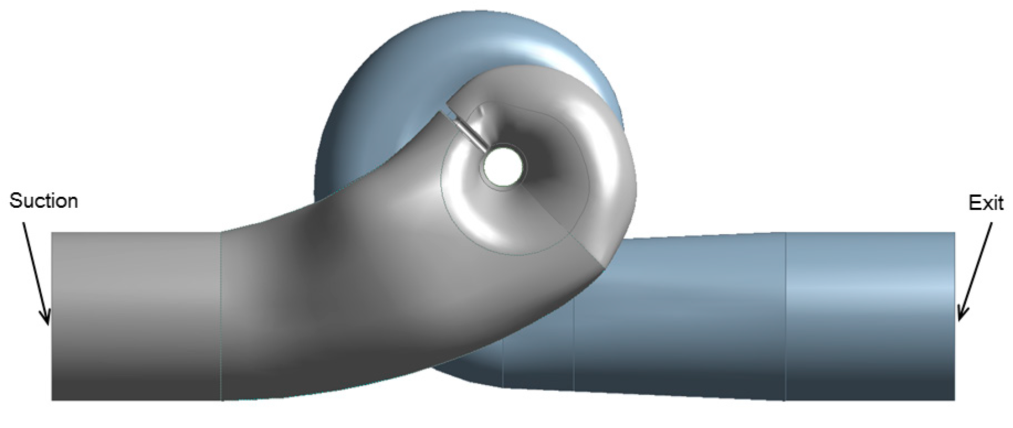
The full model was made up of two different kinds of zones: the stationary zone for the suction and extruding chambers, and the motion zone for the impeller region. In the stationary zone, for a general scalar,
, in an arbitrary control volume,
V (m
3), the convection–diffusion-reaction (CDR) equation in its integral form can be written as Equation (3):
where
is the area vector of the faces on the control volume (m
2),
is the generic variable for solving the equation, and Γ and
are the diffusion coefficient and source term of
, respectively. In the equation of continuity,
is set as 1 and Γ is 0. However, in the momentum equation,
is the velocity component and Γ is the dynamic viscosity (kg·m
−1·s
−1). From left to right, the four items in Equation (3) represent the mass variation over time, the convection term, the diffusion term and the source term, respectively.
For the motion zone, Fluent 14.0 provided a dynamic mesh model with sliding technology [
21] to better reflect the real fluid flow under the impeller–tongue interaction. With this technology, all the nodes in impeller region rotate rigidly around the center, and the dynamic mesh zone gets connected to the stationary zone of extruding chamber through non-conformal interfaces. When the mesh rotation is updated each time, the non-conformal interfaces are also likewise updated, so the new phase difference between the impeller and tongue can be truly reflected. The general transport equation in Equation (3) also applies to the dynamic mesh model, except for the convection term, which is left out due to the consideration of the mesh’s motion. Therefore, the conservation equation for the above general scalar,
, in the motion zone can be represented by Equation (4) [
21].
where
is the mesh velocity vector of the moving mesh (m·s
−1).
As there is no shape change for all of the mesh cells during the rotation of impeller, the control volume
V remains constant, and therefore the time derivative term in Equation (4) can be simplified to Equation (5) by using first-order backward difference.
where
n denotes the respective value at the nth time level, and
n + 1 represents its next time level.
For the turbulence model, the
k-
ω-based shear-stress transport (SST) model developed by Menter [
22] was used to solve the mass and momentum conservation equations. The
k-
ω-based SST model is especially well-suited for the turbulence problems occurring in high rotational speed turbomachinery due to its reasonable balance between the computational cost and accuracy. In the far field region with free shear flow, the standard
k-
ε model is used to speed up the calculations, while in the near-wall region with intense separation flow induced by the multi-curvature revolving blade walls, the turbulence model is gradually transformed into
k-
ω model to ensure the resolution of the analysis. Details of the coefficients of turbulence model can be found in a previously published report [
22].
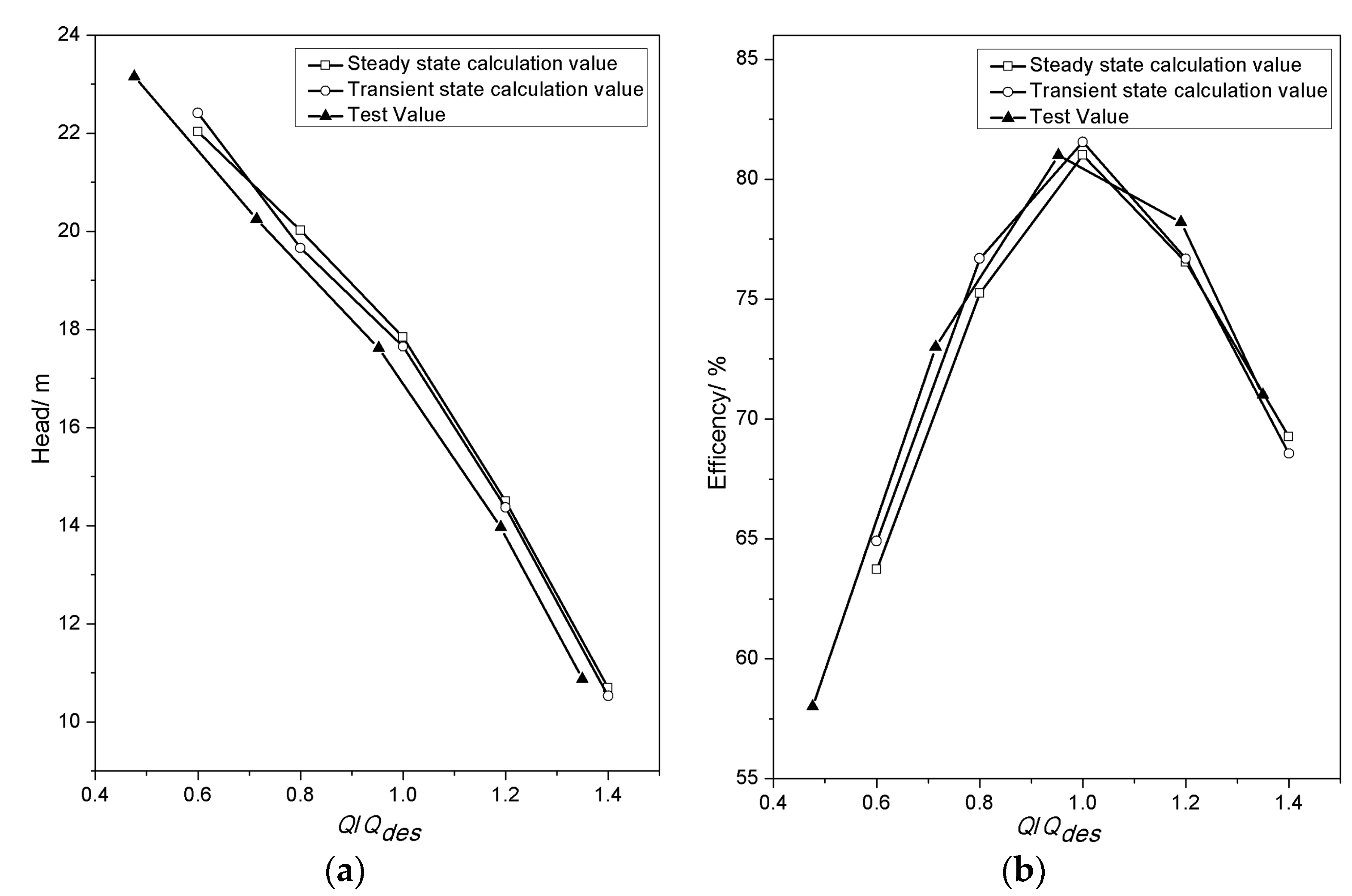
The calculation procedure was separated into two stages. The first stage was for a steady model, while the second was for an unsteady model. There were five different cases to be computed in this study, while each one corresponded to a certain working condition. The flow rates for the five cases were 0.6
Qdes, 0.8
Qdes, 1.0
Qdes, 1.2
Qdes and 1.4
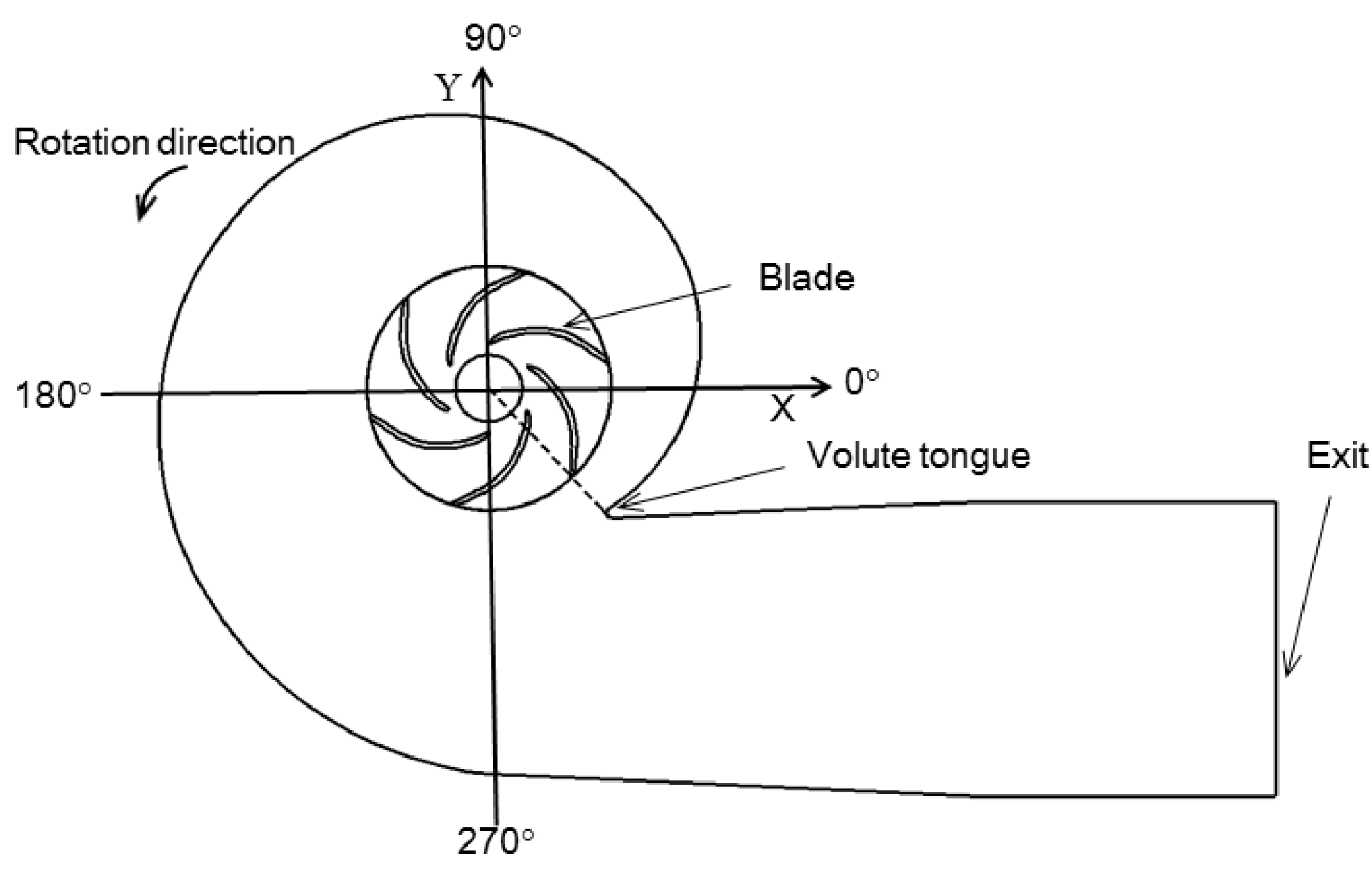
Qdes, respectively. The steady model was computed in advance to validate the calculation results with test data and then provide the initial condition for subsequent transient numerical simulation, where the impeller was located on the zero phase position. In the steady model, the full fluid region consists of two different reference frames. These reference frames were the stationary frame for the suction and extruding chambers, and the rotating frame with a rotating speed of 1480 r·min
−1 for the impeller zone. A specified flow velocity was set on the suction face as the inlet boundary condition with flow direction perpendicular to the face, and the turbulence intensity was set at 5%. An outflow condition was given on the exit face of the extruding chamber to capture the fully developed pressure and velocity distribution. All interior faces of the fluid region consisted of no-slip rough walls, and according to the specifications of the processing technology, the roughness of the blades and other faces were set to be 5 × 10
−5 m and 10
−4 m, respectively. The internal leakage of pump was ignored for simplification. Physical property parameters of pure water, including density and dynamic viscosity at 25 °C were given as the fluid properties. The convergence criterion was less than 10
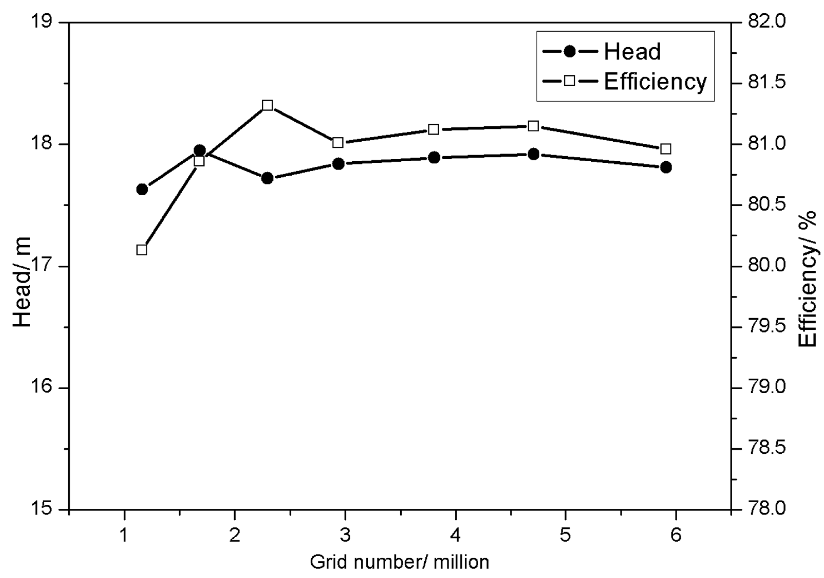
−4 for mean residues of both mass and momentum. The whole fluid region was meshed with hexahedral structure elements to ensure convergence and computational speed. To run the grid sensitivity test, seven computational cases with different mesh sizes but fixed flow rate 1.0
Qdes were studied to obtain the changes in head and efficiency values. Both the predicted head and efficiency values become very stable after the fourth point (see
Figure 3), whose rangeability becomes less than 0.3% and 0.2% respectively, so the mesh of that point was selected for computation in this work in order to save computation time. The mesh information including elements and nodes number was listed in
Table 2, and the element quality, skewness factor and orthogonal quality of the mesh was 0.73, 0.76 and 0.81 respectively. The maximum non-dimensional wall distance y+ < 60 was obtained in the full flow field of the final computation results by performing the Yplus mesh adaption refinement function [
21] during numerical computations.
2.3. Transient Calculations
After steady state computation, each case was transformed into a transient one with the steady result as its initial condition. There were mainly two differences between the unsteady and steady state models. First of all, the rotating reference frame for the impeller fluid was discarded, and a sliding mesh technique was used with a mesh motion speed of 1480 r·min
−1 to simulate the real fluid effect of the impeller’s rotation. For the solution setup, the total calculation time was 0.2432 s, corresponding to six shaft rotation cycles. The time step ∆t was defined according to the Equation (6).
where
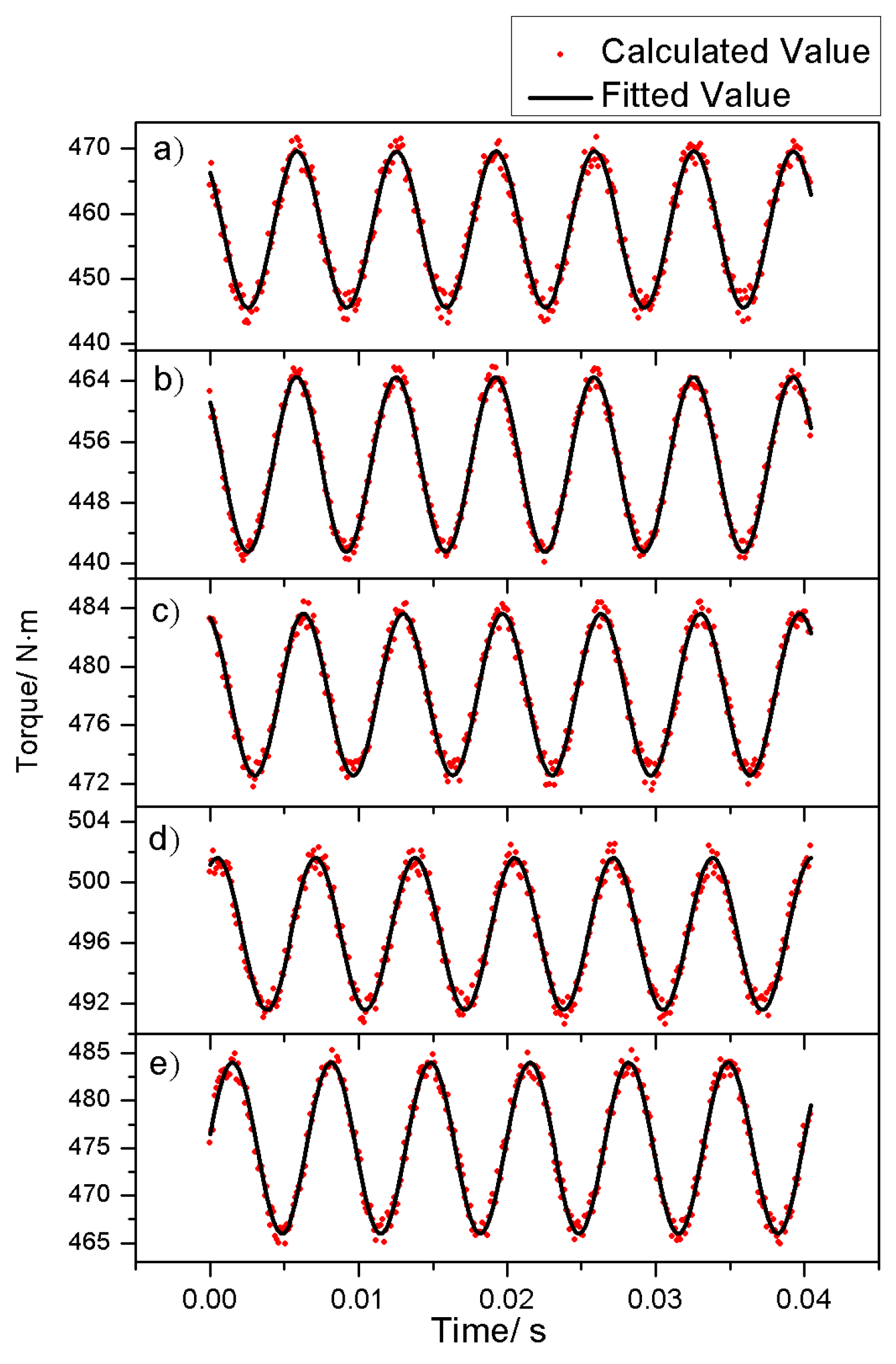
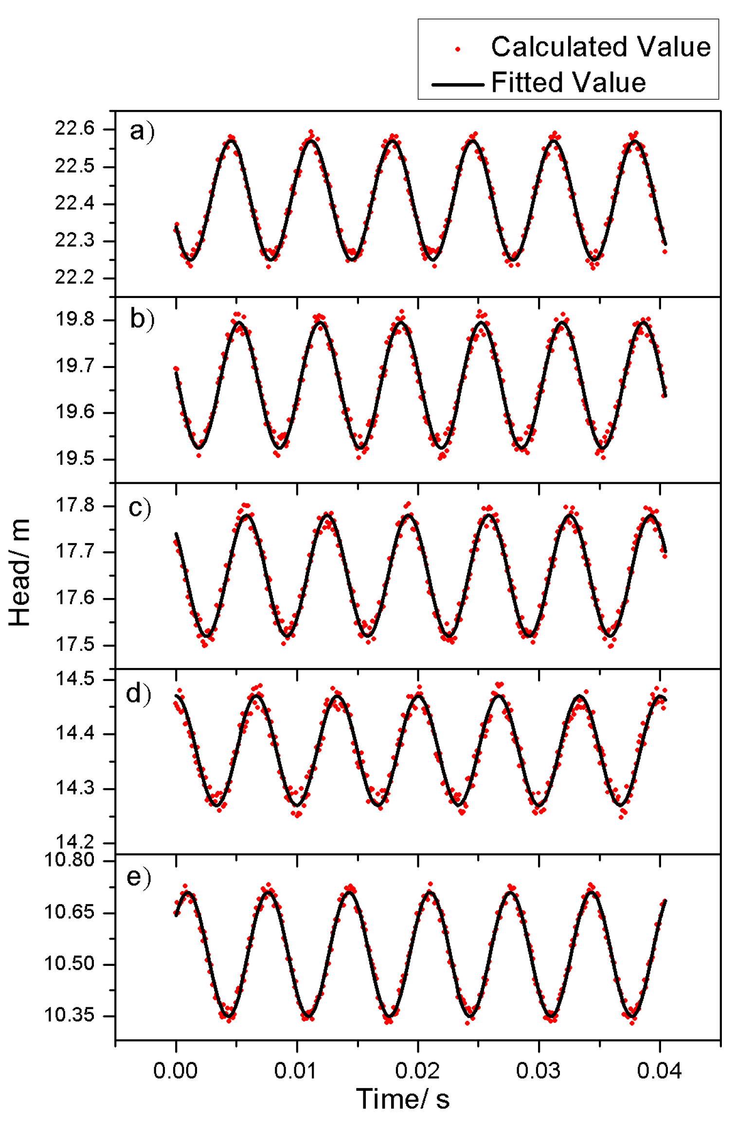
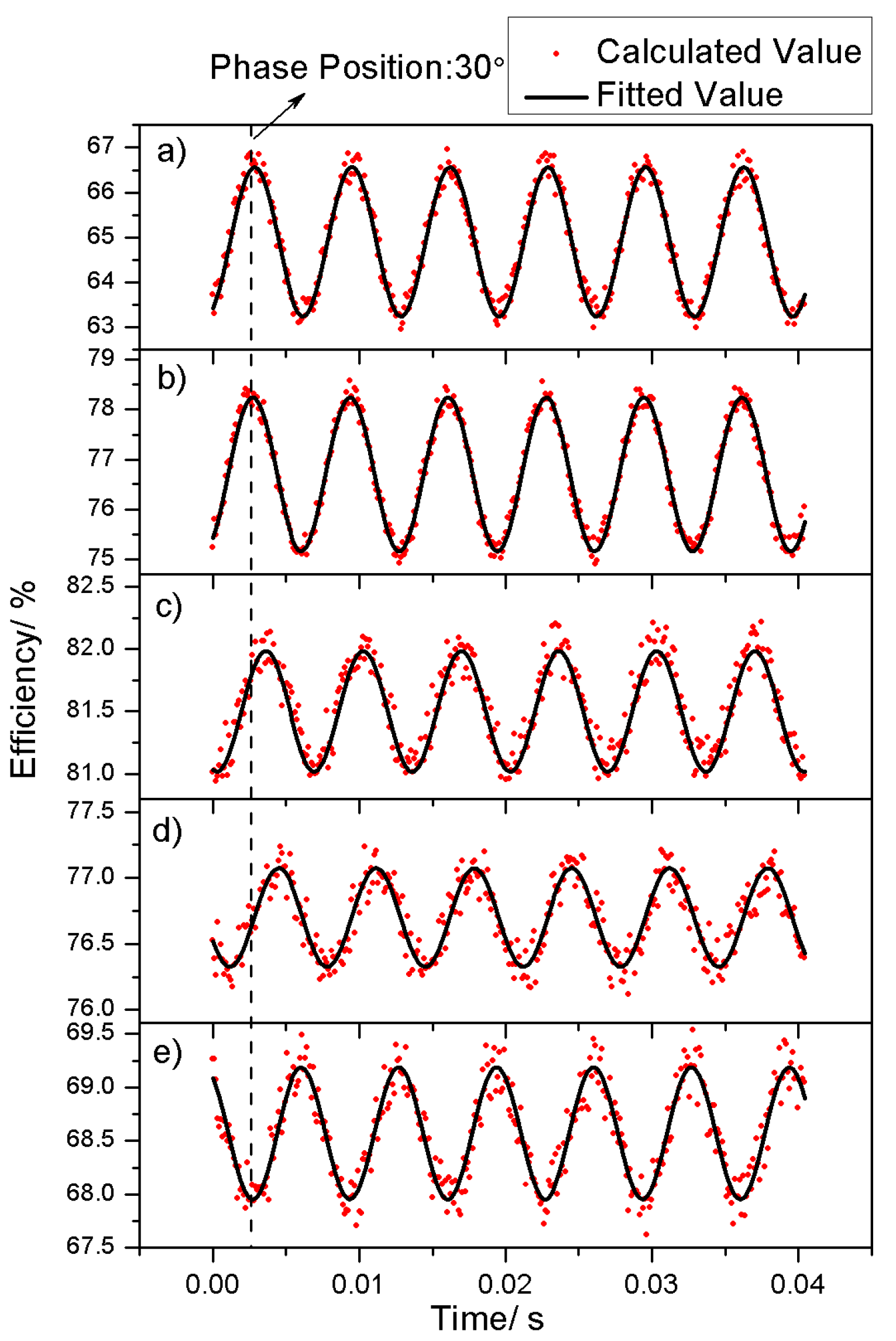
T is the rotation period of the main shaft and had the value of 0.04054 s. This means that the impeller fluid region meshes rotate 1° anticlockwise for each time step. The unsteady flow calculation results of the last shaft rotation cycle were chosen for analysis when the transient iteration was fully convergent and the fluctuation in flow parameters was regular. The head lift and fluid torque on impeller were monitored during the whole computational process, and the energy efficiency for each time step was calculated using Equation (7).
where
g is the gravitational acceleration (9.8 N·kg
−1),
Q is the volume flow rate (m
3·s
−1),
H is the head of the pump (m),
n is the shaft’s rotational speed (rev·min
−1), and
N is the torque (N·m) on the impeller. The pump head
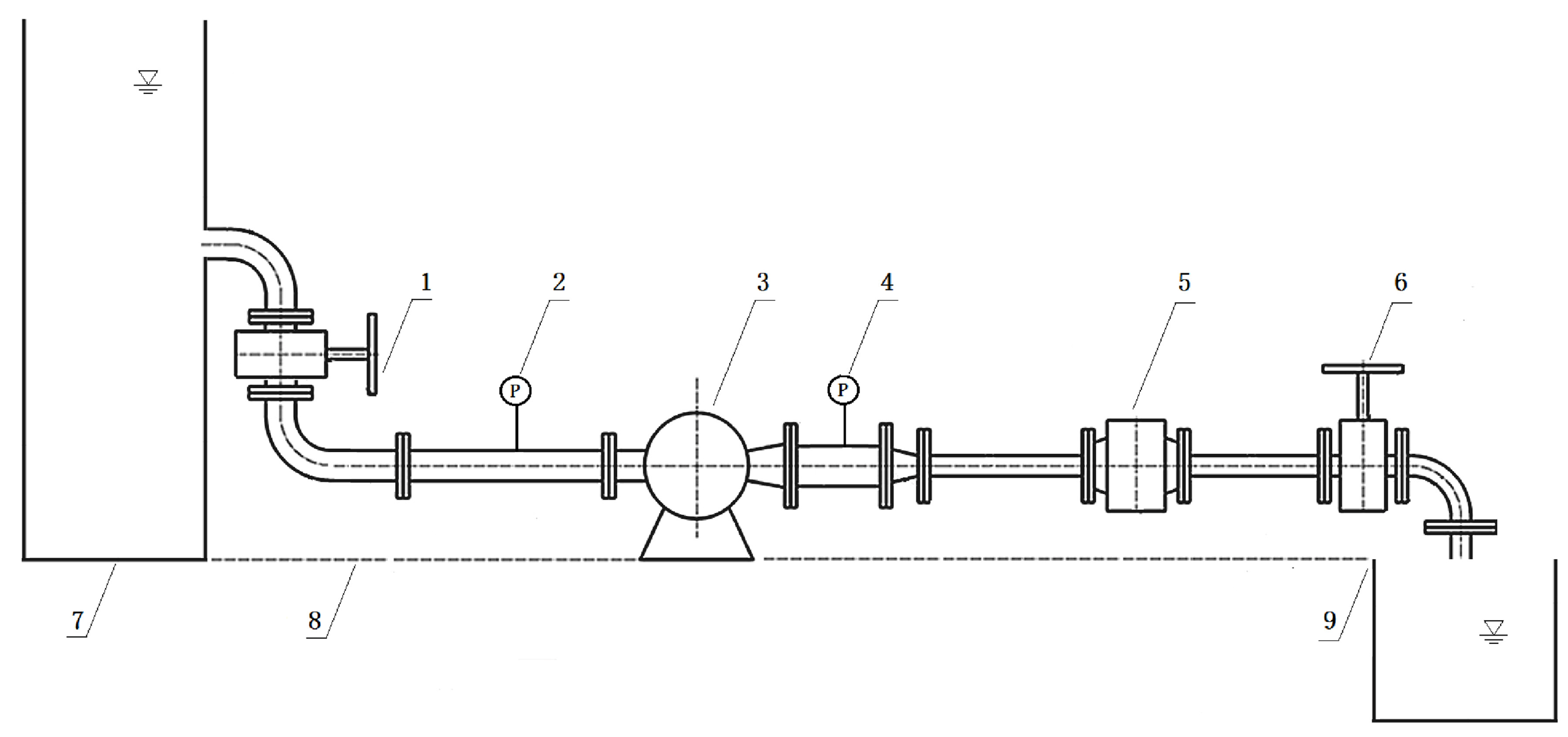
H can be obtained using Equation (8).
where
Po and
Pi represent the total pressure of the exit and entrance faces of the pump, respectively.


