Applications of Digital-Physical Hybrid Real-Time Simulation Platform in Power Systems

Abstract

Digital-physical hybrid real-time simulation (hybrid simulation) platform integrates the advantages of both digital simulation and physical simulation by combining the physical simulation laboratory and the real-time digital simulator. Based on a 400 V/50 kVA hybrid simulation platform with 500 kVA short-circuit capacity, the hybrid simulation methodology and a Hausdorff distance based accuracy evaluation method are proposed. The case validation of power system fault recurrence is performed through this platform, and the stability and accuracy are further validated by comparing the hybrid simulation waveform and field-recorded waveform and by evaluating the accuracy with the proposed error index. Two typical application scenarios in power systems are studied subsequently. The static var generator testing shows the hybrid simulation platform can provide system-level testing conditions for power electronics equipment conveniently. The low-voltage ride through standard testing of a photovoltaic inverter indicates that the hybrid simulation platform can be also used for voltage standard testing for various power system apparatus with low cost. With this hybrid simulation platform, the power system simulation and equipment testing can be implemented with many advantages, such as short period of modelling, flexible modification of parameter and network, low cost, and low risk. Based on this powerful tool platform, there will be more application scenarios in future power systems.

1. Introduction

Power system simulation is an important means to research the dynamic behavior, ensure the safety and stability, and optimize the operation of power grids. For the traditional power systems, there are lots of mature digital models and simulation experience; meanwhile, large-scale networks with high power level make it unrealistic to be simulated with actual equipment, so the real-time digital simulation maybe an ideal choice due to its advantages of fast modelling, good flexibility, and low cost. However, for the emerging new energy power generation or distributed microgrid, the digital models are not sufficient to reflect their real behaviours and characteristics and it is necessary to embed the actual devices into the digital simulation system to make simulation results more realistic. The digital-physical hybrid real-time simulation (abbreviated as hybrid simulation), also known as the power hardware-in-the-loop (PHIL) simulation, can integrate the physical simulation laboratory and digital real-time simulator [1,2,3]. Therefore, there is an increasing need to apply the hybrid simulation to the power system simulation and power equipment testing to obtain many advantages, such as short modelling period, flexible modification of network and parameter, low testing cost, and closer-to-reality simulation results.

As an advanced simulation technology, the PHIL method has been applied in many aspects. Due to the flexibility to provide various testing environment with low cost and risk, some PHIL platforms are specially designed for the control validation and testing of grid-connected inverters [4,5], motor drives [6,7], distributed energy resources (DERs) [8,9], and microgrids [10,11], etc. Based on the PHIL concept, many different kinds of converter-based emulators whose electrical behaviours are controlled to represent those of the models have been developed for the realistic and flexible testing, such as synchronous generator emulator [12], load emulator [13], induction motor load emulator [14], variable-speed wind turbine emulator [15], photovoltaic emulator [16], and energy storage emulator [17], etc. Typically, a number of emulators, each emulating a particular component, are connected together to form a hardware test bed (HTB) for the emulation of power systems [18]. In practice, the HTB can only emulate limited power network and its stability issues will be more severe due to the multiple power interfaces among the multiple emulators [2,19,20]. For the power system hybrid simulation, a power network in loop method in which the equipment can be interfaced with a digital simulator were discussed [21] and a PHIL simulation was used for laboratory education of modern power systems for the first time [22]. A remote PHIL platform using a web application core was developed for geographically-dispersed multi-site co-simulation [23]. The grid frequency regulation through energy storage resources [24] and the testing of smart grid control algorithms [25] were studied with the real equipment integrated to the simulated power system. Nevertheless, these applications involve only one emulation target or aim at systems with the complexity and the power level no more than a microgrid [12]. And there still remains the need of system-level hybrid simulation that can integrate the virtual and physical simulation systems of the power system.

To satisfy the increasing need of power system hybrid simulation and system-level equipment testing, our team have developed a 400 V/50 kVA hybrid simulation platform with 500 kVA short-circuit capacity, integrating the real-time digital simulator (RTDS) and the physical simulation laboratory [26]. As there are two types (at signal level and power level) of simulation systems interacting with each other, it could be called power system-in-the-loop (PSIL) simulation. Based on this platform, the hybrid simulation methodology and a Hausdorff distance based accuracy evaluation method are proposed. The case validation of power system fault recurrence is performed through the hybrid simulation platform, and the stability and accuracy of this platform are further validated by comparing the hybrid simulation result and field-recorded result and by evaluating the accuracy with the proposed error index. Two typical application scenarios in power systems are studied subsequently. The static var generator (SVG) is used in distribution networks to improve the voltage quality and the system-level testing of a SVG device is carried out on this platform with low cost. The related grid codes require that the grid-connected solar photovoltaic (PV) system must have the low-voltage ride through (LVRT) capability, so the LVRT standard testing of a PV inverter is conducted on this platform, which also shows that the hybrid simulation platform can be used for voltage standard testing of various power system apparatus. When implementing the power system simulation and equipment testing, the hybrid simulation platform has many advantages, such as short period of modelling, flexible parameter and network modification, low cost, and low risk. Based on this powerful tool platform, there will be more possible application scenarios in future power systems.

2. Digital-Physical Hybrid Real-Time Simulation Platform and Accuracy Evaluation Method

2.1. Overview of the Hybrid Simulation Platform

Figure 1 shows the layout of the hybrid simulation platform, including three parts: the RTDS, power interface, and physical simulation laboratory.

The RTDS is capable for the digital simulation of large-scale power grids with good flexibility. The time step of 50 μs can meet the need of real-time simulation of large-scale power grids, and the small time-step of 2~3 microseconds can be used for power electronics components. The GTAI (giga-transceiver analogue input) and GTAO (giga-transceiver analogue output) cards integrating 16-bit A/D and D/A integrating 16-bit A/D and D/A converters can be used to feed back the measured signals and send the voltage reference, respectively.

The power interface is used for power amplification, i.e., the output tracks the voltage reference from the RTDS. The power interface consists of three single-phase portions with three-phase four-wire connection at the output terminal to support the simulation of unbalanced power systems. All the employed insulated gate bipolar transistor (IGBT) modules have high switching frequency of 20 kHz. There are current and voltage measurements at the output terminal. The designed short-circuit capacity of this platform is 500 kVA, which can meet the requirements of most current application scenarios. If the higher capacity is required, the power interface needs to be expanded conveniently by adding the quantity in parallel. The detailed research and development of this platform can be found in [26].

The physical simulation laboratory is used for physical simulation. Currently the laboratory with the 800 V rated voltage has equipped with scale-down synchronous generators, transmission lines, loads, wind power, PV power, and power electronics equipment, etc. Surely, other customer products can be easily connected to the laboratory for tests if necessary. The equipment in the laboratory can be operated and monitored remotely with automation systems.

The hybrid simulation of power systems generally includes various transient phenomena and short-circuit faults, which lead to severe stability issues, so an improved interface algorithm based on ideal transformer model (ITM) is used to enhance the stability performance [27]. Meanwhile, the output DC component of the power interface is eliminated by a proper strategy, thereby improving the simulation accuracy and security [28].

2.2. Methodology for Hybrid Simulation

There are two major concerns when implementing the PSIL simulation of power systems. The first concern is how to choose an appropriate decoupling point to divide the original system into two parts, named as digital subsystem and physical subsystem, respectively. There are two general principles that should be taken into consideration. The first one is that according to the equivalent impedances, which may change during short-circuit faults, of the two subsystems, the stability condition [20] of hybrid simulation must be ensured even during various transient phenomena and short-circuit faults. The second principle is that the section of interest or with insufficient digital models should be divided into the physical subsystem. Because the actual controller and measurement of the physical model can be employed, which makes the simulation results more real. On the contrary, if there is no physical model available, the section should be divided into digital subsystem.

The second concern is to define the scale factors. Usually the physical models are scale-down, and their rated voltage and power level are fixed once they are established. However, in different applications, the same physical models may be used to simulate the real network with different voltage or power level. Therefore, there are scale factors between the physical model and the real network. The scale factors of voltage, current, apparent power, and impedance are defined as follows.

$$M_U=\frac{U_p}{U_r}$$

(1)

$$M_I=\frac{I_p}{I_r}$$

(2)

$$M_S=\frac{S_p}{S_r}=\frac{U_p{I}_p}{U_r{I}_r}=M_U\cdot M_I$$

(3)

$$M_{\left|Z\right|}=\frac{\left|Z_p\right|}{\left|Z_r\right|}=\frac{U_p}{I_P}\cdot \frac{I_r}{U_r}=\frac{M_U}{M_I}$$

(4)

where U, I, S are the root mean square (RMS) values of the voltage, current, and apparent power, respectively. |Z| is the magnitude of impedance. The subscript p and r mean the physical model and real network, respectively.

For these four scale factors, as long as any two of them are determined first, the other two scale factors will be derived. In general, the M_U is determined first according to the voltage level, then the M_S or M_|Z| according to the actual needs.

After the determination of appropriate decoupling point and scale factors, the digital subsystem will be modelled in the RTDS with true scale for virtual digital simulation, and the physical subsystem will be established by the scale-down physical devices in the laboratory for physical simulation. The terminal voltage reference from RTDS will be scaled by M_U and then sent to the power interface and amplified to drive the physical subsystem. The current and voltage at the output terminal of power interface will be scaled by 1/M_I and 1/M_U, respectively, and then fed back to the RTDS for closed-loop simulation and other control.

2.3. Proposed Accuracy Evaluation Method for Hybrid Simulation

The hybrid simulation needs to be accurate to truly reflect the behavior of the systems. For the accuracy evaluation, as the causes of hybrid simulation errors include time delay and noise injection, etc., the common quantitative indexes based on curve errors may be not reasonable enough. This paper proposed a practical evaluation method based on the Hausdorff distance theory to obtain the maximum degree of error between the reference waveform and hybrid simulation waveform. The Hausdorff distance is a measure of dissimilarity between two finite point sets and is commonly used in medical image segmentation and registration [29,30]. Herein, the Hausdorff distance is adopted for waveform comparison and its mathematical definition is as follows.

Given two finite point sets $A=\{a_1,a_2,\cdots ,a_q\}$ and $B=\{b_1,b_2,\cdots ,b_q\}$, calculate the euclidean distance between a point a_i in set A and every point in set B and find the point b_j closest to point a_i, i.e.,

$$\underset{b\in B}{\min }\Vert a_i-b\Vert =\Vert a_i-b_j\Vert \le \Vert a_i-b_k\Vert ,1\le k\le q\mathrm{and}k\ne j$$

(5)

where $\Vert \cdot \Vert$ is the euclidean distance between two points. (5) measures the minimum distance from point a_i to set B.

For all elements in set A, the maximum value that satisfies (5) is defined as the directed Hausdorff distance from set A to set B, i.e.,

$$h(A,B)=\underset{a\in A}{\max }\underset{b\in B}{\min }\Vert a-b\Vert .$$

(6)

Similarly, the directed Hausdorff distance from set B to set A is

$$h(B,A)=\underset{b\in B}{\max }\underset{a\in A}{\min }\Vert a-b\Vert .$$

(7)

The Hausdorff distance between set A to set B is defined as the maximum of h(A,B) and h(B,A), i.e.,

$$H(A,B)=\max (h(A,B),h(B,A)).$$

(8)

Thus, the H(A,B), also called the bidirectional Hausdorff distance, measures the degree of mismatch between two point sets by measuring the distance between the point in set A that is farthest from any point in set B and its nearest neighbor in set B and vice versa.

Based on the Hausdorff distance of the reference waveform and hybrid simulation waveform, a quantitative error index E is given by

$$E=\frac{H(A,B)}{\left|M\right|}\times 100\%$$

(9)

where |M| is the amplitude of waveform during steady state.

The waveforms are generally recorded as actual values with the sampling time, so the waveform data need to be normalized to eliminate the adverse effects of different quantitative scales. Supposing the sampling value and time of the waveform are both normalized in the range of [0, 1], then

$$E=\frac{H(A,B)}{\left|M\right|}\times 100\%=H(A^{\ast },B^{\ast })\times 100\%$$

(10)

where H(A^∗,B^∗) is the Hausdorff distance using the normalized waveform data.

By dividing the waveform data into different point sets according to the sampling time, the accuracy evaluation can be performed in segments, such as steady-state error and transient error. As the conditions of the each phase cannot be identical, such as power amplification, time delay, noise, and asymmetrical systems, etc., the accuracy evaluation also needs to be performed separately in phase.

3. Case Validation Based on Fault Recurrence of Power Systems

The single phase-to-ground fault is a common short circuit fault in power systems and the field-recorded waveforms can be taken as the reference waveform for the case validation of this hybrid simulation platform. Fault recurrence is one of the effective means to analyze power system faults, which is usually performed by pure digital simulation or physical simulation. This paper provided a new fault recurrence method through the hybrid simulation platform to obtain many advantages, such as short modelling period and flexible modification of network and parameter. Meanwhile, by comparing the hybrid simulation result and field-recorded result and evaluating the accuracy with the proposed error index, the stability and accuracy of this platform were further validated, which provided a reliable foundation for more applications.

3.1. Case Description and Modelling

Figure 2 shows the hybrid simulation system that is used for the two cases. The original system is composed of three substations, two power plants, two equivalent systems, all with the rated voltage of 220 kV, as well as a 110 kV substation S1. Because the short circuit faults occurs near the substation S1, only the downstream network of S1 is given in detail, and the downstream networks of other substations and power plants are replaced by equivalent loads. At the same time, the rest of networks in this area are replaced by two equivalent systems, as the electrical distance from the fault points is far enough. The lumped parameters of transmission lines are also given in Figure 2. The original system is decoupled at 10 kV BUS1 of substation S1. The digital subsystem contains most of the 220 kV networks, and the physical subsystem contains three electric cables, as well as loads. Case I is a phase-B-to-ground fault in the physical subsystem with duration of 564.4 ms. The electric cable L1 is 12.2 km in length, and the short circuit fault happens at about 35% point of the L1, near the 10 kV BUS1. Case II is an instantaneous phase-B-to-ground fault in the digital subsystem with duration of 64 ms due to the lightning strike. The fault happens at the 110 kV transmission line 1.2 km from the substation S2.

The digital models of the digital subsystem are modelled in the RTDS, and the parameters are set based on actual power system operating data. The electric cable is simulated by the reactor and resistor. The modelling of three cables is similar, so only the modelling of L1 is presented in the paper as an example. Figure 3 shows the reactor X_L and its equivalent circuit. Because the impedance angle of reactor does not match that of the actual cable, a 3.6 Ω resistor is in series with the reactor.

Table 1. Parameters of actual and simulated cable L1.

	Resistance (Ω)	Reactance (Ω)	Impedance (Ω)
Actual cable L1	1.58	1.049	1.897∠33.58°
Reactor XL	0.2843	2.28	2.298∠82.89°
Simulated cable L1 (R + XL)	3.8843	2.28	4.504∠30.41°

shows the model parameters of actual and simulated cable L1. The impedance angle of simulated cable is very close to that of actual cable, which can meet the requirement of accuracy. Meanwhile, a scale factor is needed to match the actual impedance magnitude.

Then determine the scale factors. For the single phase-to-ground fault, the voltage of non-fault phase is higher than the rated voltage. Thus, the rated voltage of physical subsystem in the laboratory is chosen to be 320 V, i.e., the 10 kV actual system is simulated by 320 V physical subsystem. The short circuit fault can only be set at both ends of the reactor, so the reactor can only simulate the short circuit impedance during the faults, i.e., the reactor and resistor can simulate 35% of the electric cable. Therefore, the scale factors are determined as follows.

M_U = 320 V/10 kV = 0.032

M_|Z| = 4.504 Ω/(1.897 × 0.35) Ω = 6.7836

M_I = M_U/M_|Z| = 0.004717

M_S = M_U × M_I = 0.0001509

The scale factor M_U and M_I are set at the signal processing section in RTDS to covert the scale of reference voltage and feedback current, respectively.

The fault recurrence application has been carried out with the hybrid simulation method and the results of the above two cases are presented subsequently.

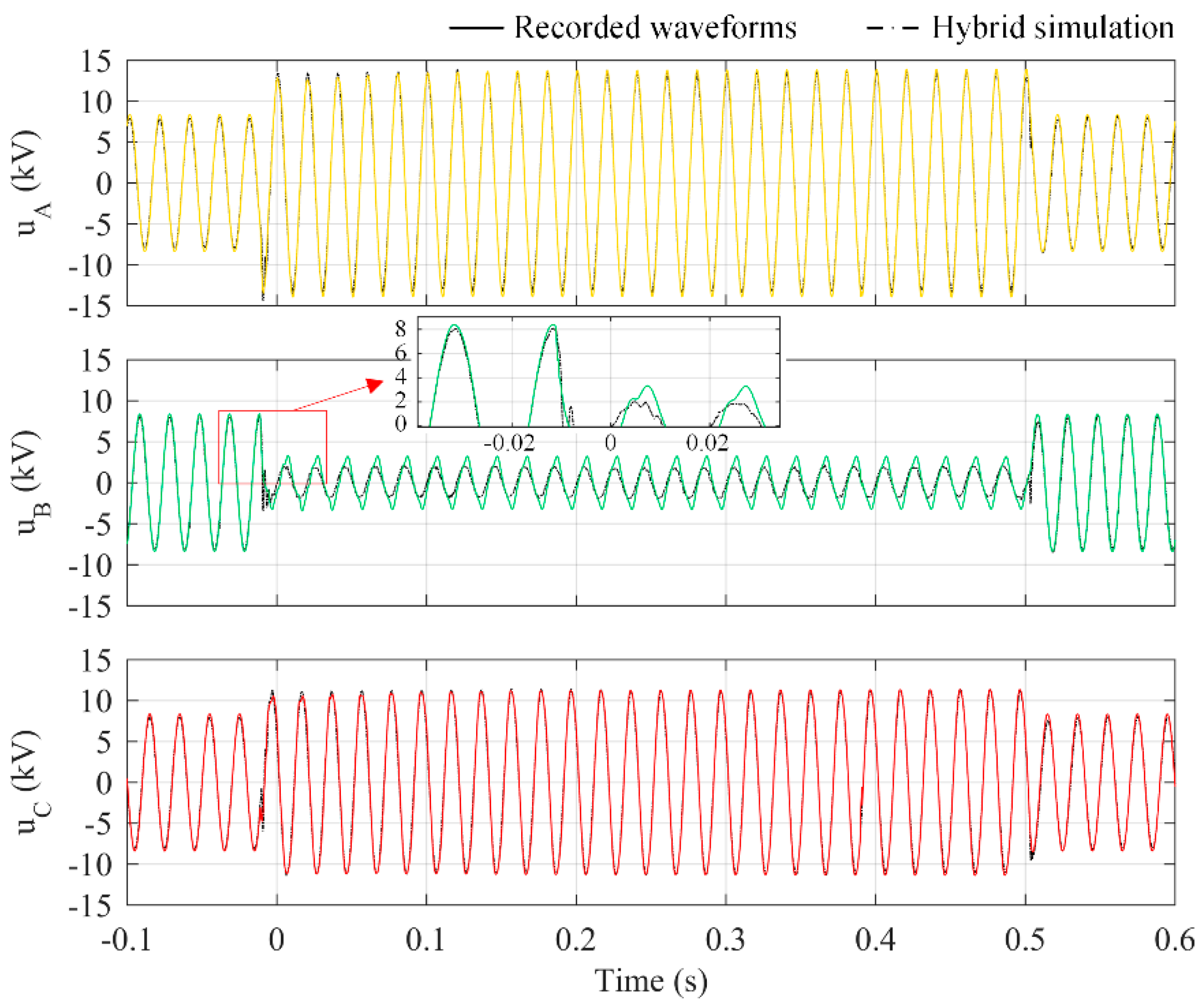
3.2. Result of Case I

Case I is a phase-B-to-ground fault occurring on the cable L1 for 564.4 ms and the fault point is set at the point F_p in the physical subsystem. Before conducting the fault recurrence application, it is necessary to set an accurate initial fault voltage angle (abbreviated as fault angle). The three-phase fault voltage waveforms at the 10 kVA BUS1 were recorded by the fault recorder in the field and the fault angle is about 219.6° according to the fault waveforms. When conducting the hybrid simulation, the fault angle needs to be adjusted by a fault angle controller and the results are closer to the recorded waveforms when the fault angle is set as 223.2°. Figure 4 shows the waveform comparisons between the recorded fault voltages and hybrid simulation voltages measured at BUS1.

Table 2. Accuracy evaluation results of case I.

	E_Stable (−0.1~−0.0114 s)	E_Fault (−0.0112~0.502 s)	E_All (−0.1~0.6 s)
Phase A	3.28%	4.51%	4.51%
Phase B	2.50%	8.76%	8.76%
Phase C	2.81%	4.19%	4.19%

shows the accuracy evaluation results. The three error indexes of each phase are calculated using three different data segments, i.e., the steady state, fault duration, and all waveform, respectively. The hybrid simulation waveforms are substantially coincident with the field-recorded waveforms and the error indexes are less than 10%, which indicates the platform is of high accuracy. The fault angle controller cannot control the fault angles with absolute accuracy, which causes small errors in the fault angle; however, it does not matter as the fault angle can be adjusted repeatedly till the simulated voltage is very close to the recorded voltage.

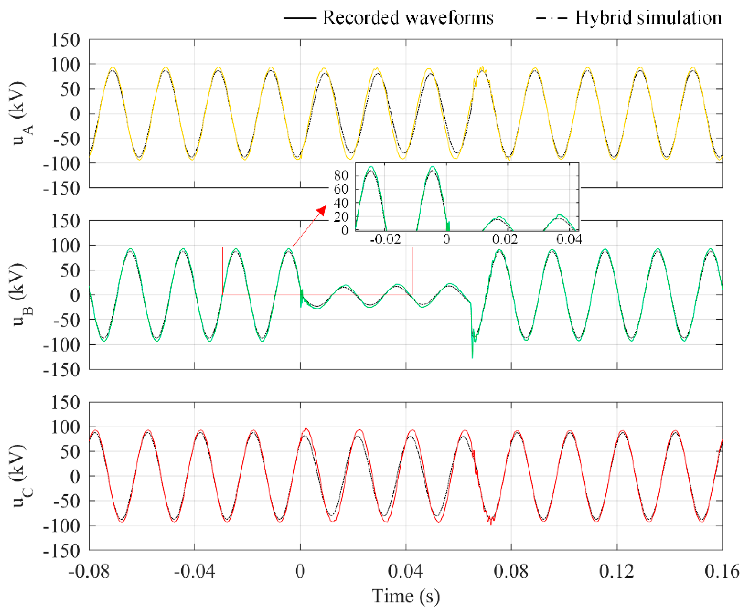
3.3. Result of Case II

Case II is a phase-B-to-ground fault occurring in the digital subsystem for 64 ms and the fault is set at point F_d in the RTDS. According to the three-phase voltages recorded at the 110 kV side of the substation S2, the fault angle is 288°. Figure 5 shows the waveform comparisons of recorded voltages and the hybrid simulation voltages measured at 110 kV side of substation S2, and

Table 3. Accuracy evaluation results of case II.

	E_Stable (−0.08~−0.0002 s)	E_Fault (0~0.0646 s)	E_All (−0.08~0.16 s)
Phase A	3.50%	7.03%	7.03%
Phase B	3.23%	4.11%	23.12%
Phase C	3.27%	8.01%	8.01%

gives the accuracy evaluation results. The three error indexes of each phase are calculated using three different data segments, i.e., the steady state, fault duration, and all waveform, respectively. The hybrid simulation waveforms are substantially coincident with the field-recorded waveforms and the error indexes are less than 10% (except the abnormal 23.12%), which indicates the platform is of high accuracy. Herein, by changing the value of the grounding resistance, the voltage of fault phase is close to the recorded one. The voltages of the non-fault phases are with slightly large errors, which means the physical model parameters of non-fault phases of transmission lines differ more from those of the actual transmission lines. The abnormal E_all of phase B is too large (23.12%) due to the large oscillation of the recorded waveform at the end of the fault.

The results of fault recurrence of power system are close to the corresponding field-recorded waveforms, which indicates that this digital-physical hybrid simulation platform is of high accuracy and the hybrid simulation method is effective. The successful application of the fault recurrence provides the reliable foundation and important guarantee of stability and accuracy for more power system applications.

4. System-Level Testing of SVG

With the development of power systems, there are more and more power electronics devices being employed to improve the power quality and control flexibility. The SVG, also called static synchronous compensator (STATCOM), is a kind of reactive power compensation device with fast and continuous compensation characteristics. The SVG is used in the low-voltage distribution networks to improve the voltage quality. Any new devices need to be fully tested before connecting to the power grid. The digital-physical hybrid simulation platform can easily provide various testing environment with low cost, so the system-level testing of a SVG device has been carried out on this platform, which mainly focuses on the effects of SVG on the distribution network, such as unbalanced load compensation and short-circuit fault support.

Figure 6 shows the SVG testing system. The digital subsystem is composed of a simplified 10 kV network to provide variable testing conditions, such as different voltage ranges and short-circuit faults. Of course, the more completed network can conveniently be built in the digital subsystem if necessary. The physical subsystem is built in the lab, and the parameters of SVG and other components are given by

Table 4. Parameters of physical subsystem used for SVG testing.

Component	Parameter	Value
SVG	Rated voltage	400 V
	Rated capacity	50 kvar
Line-simulating reactor (31XL)	Impedance	8.608∠50.45° Ω
Cable-simulating reactor (34XL)	Impedance	1.14∠82.9° Ω
Load (91~94RLD, identical)	Resistive load (R)	70 Ω
	Impedance load (L)	152.315∠23.2° Ω
	Dynamic motor (D)	5 kVA
Unbalanced load (Resistive)	Phase A	5 Ω
	Phase B	8 Ω
	Phase C	11 Ω

. Every load can be switched individually. The reactor 31X_L is used to simulate an actual transmission line with a reasonably assumed impedance of 2.12∠50.45 Ω.

Therefore, the scale factors are as follows.

M_U = 380 V/380 V = 1

M_|Z| = 8.608 Ω/2.12 Ω = 4.0604

M_I = M_U/M_|Z| = 0.2463

M_S = M_U × M_I = 0.2463

The full tests of a SVG device have been done with the hybrid simulation system and this paper will present partial testing results, including SVG input voltage range testing, compensating unbalanced load testing and compensating short-circuit fault testing.

4.1. SVG Input Voltage Range Testing

This low-voltage SVG device is generally installed at the sensitive load for voltage compensation. According to its data sheet, the normal input phase voltage of SVG is 138~265 V and the SVG will alarm and stop if the input voltage is out of the range. Therefore, the input voltage range testing is very important for the normal and safe operation of SVG device. The SVG is connected to the 380 V bus and operates in a constant power factor mode. By changing the power voltage in the RTDS, the voltage of 380 V bus in the physical subsystem will change accordingly to complete the input volte range testing.

Table 5. Results of SVG input voltage range testing.

No.	Loads	Input Phase Voltage (V)	Output Reactive Power (kvar)	SVG State
1	91-92RLD	209	5.61	Normal
2	91-93RLD	205	6.95	Normal
3	91-94RLD	205	7.80	Normal
4	91-94RLD	192	6.96	Normal
5	91-94RLD	174	5.98	Normal
6	91-94RLD	160	5.13	Normal
7	91-94RLD	152	4.62	Normal
8	91-94RLD	138.5	3.88	Normal
9	91-94RLD	136	3.75	Normal
10	91-94RLD	134	0.325	Warning

gives the results of low-voltage range testing. The high-voltage range testing is similar and is not presented in this paper. Due to the constant power factor mode, the SVG outputs more reactive power when the loads increase. With the decrease of bus voltage, the reactive loads gradually reduced and the SVG outputs less reactive power. When the input phase voltage is 134 V, the SVG device stops running and alarms automatically because of its low-voltage protect control. The SVG device passes the input voltage range testing.

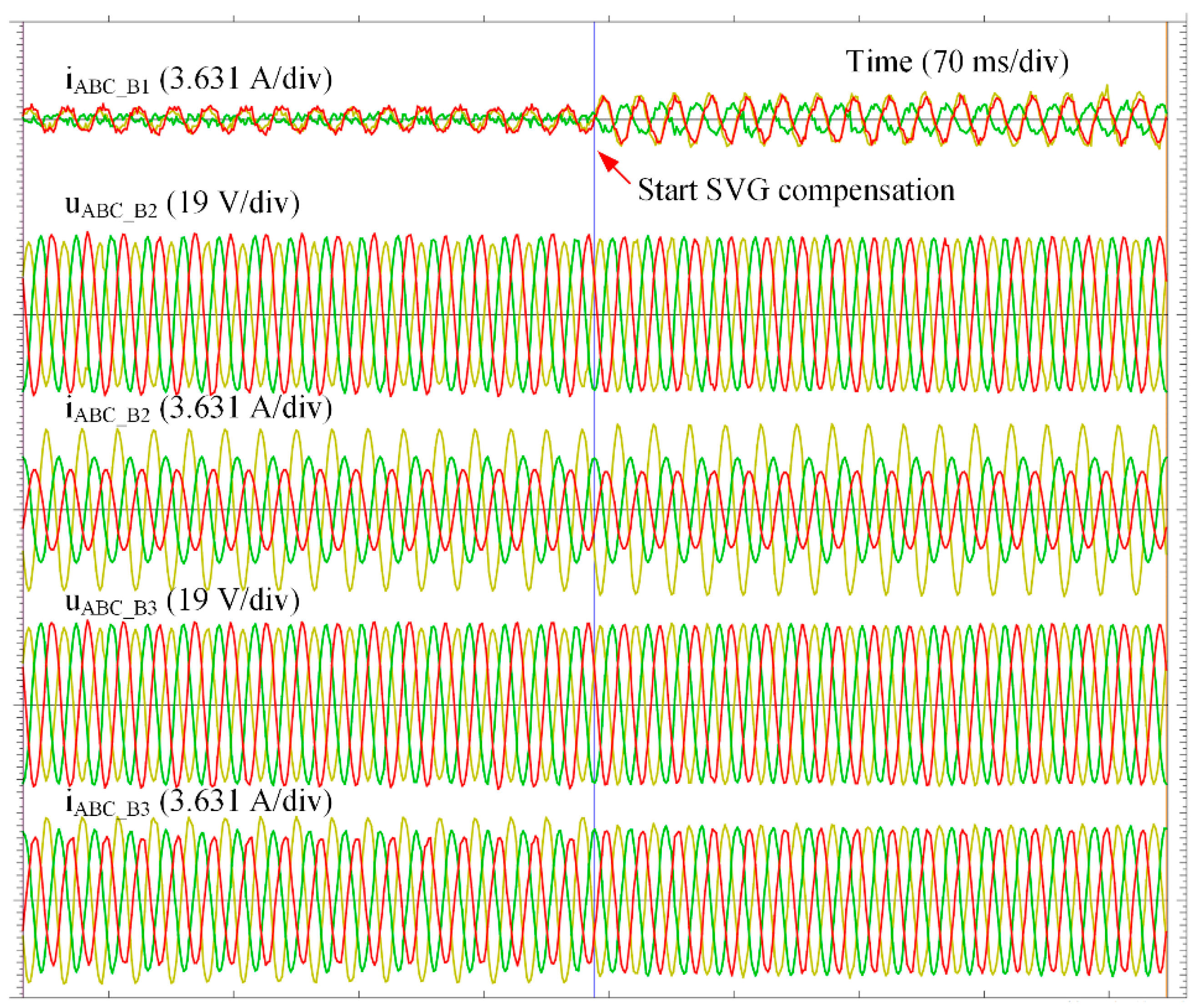
4.2. Compensating Unbalanced Load Testing

The SVG device has the function of compensating unbalanced currents caused by the unbalanced loads. When conducting this testing, the operation mode of the SVG device is set to be three-phase unbalanced compensation mode. The 91RLD, 92RL, and unbalanced loads are put into operation at first and the SVG is disabled, so the testing system is under an unbalanced state. Then the SVG is enabled to compensate unbalanced loads. Figure 7 shows the three-phase voltage and current waveforms measured at breaker B1, B2, and B3, respectively, and the three-phase voltages and currents (RMS values, similarly hereinafter) measured at breaker B3 are given by

Table 6. Three-phase voltages and currents measured at breaker B3 with unbalanced loads.

SVG	VA_RMS (V)	VB_RMS (V)	VC_RMS (V)	IA_RMS (A)	IB_RMS (A)	IC_RMS (A)
Disabled	162	177.12	187.36	36.06	27.96	22.66
Enabled	174.4	174.4	175.8	30.36	30.32	29.42

. Therefore, the voltages and currents at B3 almost become balanced after the SVG is put into operation, which shows the SVG can compensate the three-phase unbalanced loads well.

4.3. Compensating Short-Circuit Fault Testing

The short-circuit faults occurred in the power systems will have influence on the loads. The SVG can provide reactive power to support the load voltage so as to reduce the impacts of short-circuit faults on the loads. Therefore, the tests of SVG compensation for short-circuit fault were carried out. The short-circuit fault point is set at point F in the digital subsystem, as shown in Figure 6, and the tests under various types of short-circuit fault were completed. As the situations under different short-circuit faults are similar, only the testing results of single phase-to-ground fault are presented in this paper.

As there is no power source in the physical subsystem, the single phase-to-ground fault is set with a 10 Ω grounding resistor and lasts 0.5 s. The 91RL and 92RL loads are connected in parallel with the SVG device. For comparison, two tests were carried out. In the first test, the SVG device does not operate, and the SVG device is put into operation in the second test. Figure 8 shows the three-phase voltages and reactive power measured at breaker B1 (the output terminal of SVG device). It should be pointed out that the fault voltages are measured at the star side of the transformer but the fault happened at the delta side of the transformer. With the SVG compensation, the three-phase load voltages during the fault are 198.17 V, 168.96 V, and 206.08 V, respectively. However, without the SVG compensation, those voltages are 208.99 V, 152.70 V, and 206.78 V, respectively. The results show that the SVG can provide some support to the load voltage drop of the fault phase by providing reactive power compensation during the fault. Through the SVG testing scenario, it appears that the platform can provide a low-cost system-level testing method for various power electronics devices owing to the fact that large-scale power systems can be modelled in digital subsystem easily.

5. Low-Voltage Ride through Standard Testing of PV Inverter

With the increasing penetration of renewable energy resource in the power grid, the related grid codes require that the grid-connected solar PV system must have the low-voltage ride through capability so that the PV system remains connected to the grid during voltage sags for a specific period of time to provide grid support during grid faults [31,32]. The grid-connected inverter of a PV system should be able to detect the fault incident and more importantly react quickly to ensure the LVRT capability. Therefore, we tested the LVRT capability of a kind of grid-connected PV inverter using the hybrid simulation platform.

5.1. Testing System

The LVRT characteristics vary from country to country with small changes in voltage sag magnitude, recovery time, and final voltage magnitude [32]. According to the relevant codes, the testing standard of LVRT testing of PV inverter is shown in Figure 9. The time 0 s is the moment when the fault occurs and the PV system must remain connected to the grid above the green line.

Figure 10 shows the hybrid simulation system used for the LVRT standard testing of PV inverter. The programmable voltage source in the digital subsystem is used to set different voltage sags. The PV source is simulated by the 10 kW monocrystalline silicon array installed on the roof of the laboratory. The PV inverter is rated at 30 kW and 398 V (phase voltage 230 V) with three-phase four-wire connection at the output terminal and connected to the 800 V bus through a step-up isolation transformer. The 21~23X_L are line-simulating reactors without parallel capacitors and are with impedances of 17.027∠86.03° Ω, 8.44∠86.4° Ω, and 16.88∠86.4° Ω, respectively. The load parameters of 91~94RL are given in Table 4.

As this testing system does not exist magnitude conversion of voltage or current between the two subsystems, all the scale factors are 1. The different testing conditions, including sag magnitude, symmetry and duration time, can be realized easily and conveniently by setting the programmable voltage source and then detect whether the PV inverter remains connected.

5.2. Results of LVRT Standard Testing

According to the LVRT standard, the various tests under different voltage sag conditions have been carried out. The voltage sag range includes 80%, 50%, and 20% of the rated voltage. At every voltage magnitude, it also includes three-phase, two-phase, and single-phase voltage sag. The corresponding duration time of voltage sag is set as that of the requirement of LVRT standard. The testing results are given by

Table 7. LVRT standard testing results of PV inverter under different voltage sags.

Magnitude (p.u.)	Phase	Duration Time (s)	Remain Connected	Pass Test
80%	Three phases	1.55	Yes	Yes
	Two phases	1.55	Yes	Yes
	Single phase	1.55	Yes	Yes
50%	Three phases	1.1	Yes	Yes
	Two phases	1.1	Yes	Yes
	Single phase	1.1	Yes	Yes
20%	Three phases	0.625	Yes	Yes
	Two phases	0.625	Yes	Yes
	Single phase	0.625	Yes	Yes

, which shows that the PV inverter passed the LVRT testing and could meet the LVRT standard.

The line voltage and line current waveforms of the PV inverter output terminal were measured during tests. Due to limited pages, only the testing waveforms under three-phase 80% sag, two-phase 50% sag, and single-phase 20% sag are presented in this paper. The other testing waveforms under different conditions are similar. Figure 11 shows the output three-phase line voltage and line current waveforms of PV inverter under the above three conditions. It should be pointed out that the voltage sags are set near the star side of the transformer but the waveforms are measured at the delta side of the transformer. During the voltage sags, the three-phase output currents increase and are controlled to be symmetrical, and the PV inverter remains connected to the grid. After the voltage sags, the PV inverter returns to normal operation.

Compared with the conventional LVRT testing means, the method through this hybrid simulation platform can provide various LVRT testing conditions flexibly and conveniently with low cost. What’s more, the LVRT testing of a PV inverter can embed to a virtual power grid to research the influence of LVRT on the power grid. Through the LVRT standard testing scenario of PV inverter, it indicates that the hybrid simulation platform can be also used for voltage standard testing of various power system apparatus with low cost.

6. Conclusions

Based on the 400 V/50 kVA digital-physical hybrid real-time simulation platform with the short-circuit capacity of 500 kVA, the hybrid simulation methodology and a Hausdorff distance based accuracy evaluation method are proposed. The case validation of power system fault recurrence is performed through this platform and the stability and accuracy are further validated. The successful case validation provides the reliable foundation and important guarantee of stability and accuracy for more power system applications. The SVG testing scenario provides a low-cost system-level testing method for various power electronics devices owing to the fact that large-scale power systems can be modelled in digital subsystem easily. The LVRT standard testing scenario of PV inverter indicates that the hybrid simulation platform can be also used for voltage standard testing of various power system apparatus with low cost.

Other application scenarios can also be performed on this hybrid simulation platform. The microgrid can be connected in the physical subsystem and the related energy management strategy and new control method can be validated. Similar with the PV inverter testing, the wind power generation can be installed and be studied. For researchers specializing in the power electronics technology, the hybrid simulation platform will help them speed up the development process of emerging technology.

This hybrid simulation platform has advantages of short period of modelling, flexible modification of parameter and network, and low cost when implementing the power system simulation and equipment testing. Based on this powerful tool platform, there will be more possible application scenarios in further power systems, such as the simulation and analysis of power system and the research & development of new energy power generation, microgrid, and emerging power electronics technology.

References

1. Roscoe, A.J.; Mackay, A.; Burt, G.M.; McDonald, J.R. Architecture of a network-in-the-loop environment for characterizing AC power-system behavior. IEEE Trans. Ind. Electron. 2010, 57, 1245–1253. [Google Scholar] [CrossRef] [Green Version]
2. Lauss, G.F.; Faruque, M.O.; Schoder, K.; Dufour, C.; Viehweider, A.; Langston, J. Characteristics and design of power hardware-in-the-loop simulations for electrical power systems. IEEE Trans. Ind. Electron. 2016, 63, 406–417. [Google Scholar] [CrossRef]
3. Kotsampopoulos, P.C.; Lehfuss, F.; Lauss, G.F.; Bletterie, B.; Hatziargyriou, N.D. The limitations of digital simulation and the advantages of PHIL testing in studying distributed generation provision of ancillary services. IEEE Trans. Ind. Electron. 2015, 62, 5502–5515. [Google Scholar] [CrossRef]
4. Hoke, A.; Chakraborty, S.; Basso, T. A power hardware-in-the-loop framework for advanced grid-interactive inverter testing. In Proceedings of the 2015 IEEE Power & Energy Society Innovative Smart Grid Technologies Conference (ISGT), Washington, DC, USA, 18–20 February 2015; pp. 1–5. [Google Scholar]
5. Palmintier, B.; Lundstrom, B.; Chakraborty, S.; Williams, T.; Schneider, K.; Chassin, D. A power hardware-in-the-loop platform with remote distribution circuit cosimulation. IEEE Trans. Ind. Electron. 2015, 62, 2236–2245. [Google Scholar] [CrossRef]
6. Steurer, M.; Edrington, C.S.; Sloderbeck, M.; Ren, W.; Langston, J. A megawatt-scale power hardware-in-the-loop simulation setup for motor drives. IEEE Trans. Ind. Electron. 2010, 57, 1254–1260. [Google Scholar] [CrossRef]
7. Saito, K.; Akagi, H. A power hardware-in-the-loop (P-HIL) test bench using two modular multilevel DSCC converters for a synchronous motor drive. IEEE Trans. Ind. Appl. 2018. [Google Scholar] [CrossRef]
8. Huerta, F.; Gruber, J.K.; Prodanovic, M.; Matatagui, P. Power-hardware-in-the-loop test beds: Evaluation tools for grid integration of distributed energy resources. IEEE Ind. Appl. Mag. 2016, 22, 18–26. [Google Scholar] [CrossRef]
9. Hoke, A.F.; Nelson, A.; Chakraborty, S.; Bell, F.; McCarty, M. An islanding detection test platform for multi-inverter islands using power HIL. IEEE Trans. Ind. Electron. 2018, 65, 7944–7953. [Google Scholar] [CrossRef]
10. Wang, J.; Song, Y.; Li, W.; Guo, J.; Monti, A. Development of a universal platform for hardware in-the-loop testing of microgrids. IEEE Trans. Ind. Inf. 2014, 10, 2154–2165. [Google Scholar] [CrossRef]
11. Vijay, A.S.; Doolla, S.; Chandorkar, M.C. Real-time testing approaches for microgrids. IEEE J. Emerg. Sel. Top. Power Electron. 2017, 5, 1356–1376. [Google Scholar] [CrossRef]
12. Yang, L.; Wang, J.; Ma, Y.; Wang, J.; Zhang, X.; Tolbert, L.M.; Wang, F.F.; Tomsovic, K. Three-phase power converter-based real-time synchronous generator emulation. IEEE Trans. Power Electron. 2017, 32, 1651–1665. [Google Scholar] [CrossRef]
13. Wang, J.; Yang, L.; Ma, Y.; Wang, J.; Tolbert, L.M.; Wang, F.F.; Tomsovic, K. Static and dynamic power system load emulation in a converter-based reconfigurable power grid emulator. IEEE Trans. Power Electron. 2016, 31, 3239–3251. [Google Scholar] [CrossRef]
14. Wang, J.; Ma, Y.; Yang, L.; Tolbert, L.M.; Wang, F. Power converter-based three-phase induction motor load emulator. In Proceedings of the 2013 Twenty-Eighth Annual IEEE Applied Power Electronics Conference and Exposition (APEC), Long Beach, CA, USA, 17–21 March 2013; pp. 3270–3274. [Google Scholar]
15. Huerta, F.; Tello, R.L.; Prodanovic, M. Real-time power-hardware-in-the-loop implementation of variable-speed wind turbines. IEEE Trans. Ind. Electron. 2017, 64, 1893–1904. [Google Scholar] [CrossRef]
16. Mai, X.H.; Kwak, S.; Jung, J.; Kim, K.A. Comprehensive electric-thermal photovoltaic modeling for power-hardware-in-the-loop simulation (PHILS) applications. IEEE Trans. Ind. Electron. 2017, 64, 6255–6264. [Google Scholar] [CrossRef]
17. Seitl, C.; Messner, C.; Popp, H.; Kathan, J. Emulation of a high voltage home storage battery system using a power hardware-in-the-loop approach. In Proceedings of the 42nd Annual Conference of the IEEE Industrial Electronics Society, Florence, Italy, 24–27 October 2016; pp. 6705–6710. [Google Scholar]
18. Yang, L.; Ma, Y.; Wang, J.; Wang, J.; Zhang, X.; Tolbert, L.M.; Wang, F.; Tomsovic, K. Development of converter based reconfigurable power grid emulator. In Proceedings of the IEEE Energy Conversion Congress and Exposition, Pittsburgh, PA, USA, 14–18 September 2014; pp. 3990–3997. [Google Scholar]
19. Zhang, S.; Ma, Y.; Yang, L.; Wang, F.; Tolbert, L.M. Development of a hybrid emulation platform based on RTDS and reconfigurable power converter-based testbed. In Proceedings of the 31st Annual IEEE Applied Power Electronics Conference and Exposition, Long Beach, CA, USA, 20–24 March 2016; pp. 3121–3127. [Google Scholar]
20. Ren, W.; Steurer, M.; Baldwin, T.L. Improve the stability and the accuracy of power hardware-in-the-loop simulation by selecting appropriate interface algorithms. IEEE Trans. Ind. Appl. 2008, 44, 1286–1294. [Google Scholar] [CrossRef]
21. Goyal, S.; Ledwich, G.; Ghosh, A. Power network in loop: A paradigm for real-time simulation and hardware testing. IEEE Trans. Power Deliv. 2010, 25, 1083–1092. [Google Scholar] [CrossRef] [Green Version]
22. Kotsampopoulos, P.C.; Kleftakis, V.A.; Hatziargyriou, N.D. Laboratory education of modern power systems using PHIL simulation. IEEE Trans. Power Syst. 2017, 32, 3992–4001. [Google Scholar] [CrossRef]
23. Lundstrom, B.; Palmintier, B.; Rowe, D.; Ward, J.; Moore, T. Trans-oceanic remote power hardware-in-the-loop: Multi-site hardware, integrated controller, and electric network co-simulation. IET Gener. Transm. Distrib. 2017, 11, 4688–4701. [Google Scholar] [CrossRef]
24. Kim, Y.; Wang, J. Power hardware-in-the-loop simulation study on frequency regulation through direct load control of thermal and electrical energy storage resources. IEEE Trans. Smart Grid 2018, 9, 2786–2796. [Google Scholar] [CrossRef]
25. Maniatopoulos, M.; Lagos, D.; Kotsampopoulos, P.; Hatziargyriou, N. Combined control and power hardware in-the-loop simulation for testing smart grid control algorithms. IET Gener. Transm. Distrib. 2017, 11, 3009–3018. [Google Scholar] [CrossRef]
26. Mao, C.; Leng, F.; Li, J.; Zhang, S.; Zhang, L.; Mo, R.; Wang, D.; Zeng, J.; Chen, X.; An, R.; et al. A 400-V/50-kVA digital-physical hybrid real-time simulation platform for power systems. IEEE Trans. Ind. Electron. 2018, 65, 3666–3676. [Google Scholar] [CrossRef]
27. Zeng, J.; Leng, F.; Peng, B.; Li, J.; An, R.; Chen, X.; Mao, C.; Wang, D. A novel impedance compensation algorithm for improving the stability of digital-physical hybrid simulation. In Proceedings of the 43rd Annual Conference of the IEEE Industrial Electronics Society, Beijing, China, 29 October–1 November 2017; pp. 51–55. [Google Scholar]
28. Zeng, J.; Li, J.; Leng, F.; Peng, B.; Chen, X.; Mao, C.; Wang, D. A DC component elimination control strategy for the interface system of digital-physical hybrid real-time simulation. In Proceedings of the 43rd Annual Conference of the IEEE Industrial Electronics Society, Beijing, China, 29 October–1 November 2017; pp. 515–520. [Google Scholar]
29. Wang, A.; Sun, X.; Zhou, X.; Hu, W. Difference squared Hausdorff distance based medical image registration. In Proceedings of the 2011 23rd Chinese Control and Decision Conference, Mianyang, China, 23–25 May 2011; pp. 4270–4272. [Google Scholar]
30. Taha, A.A.; Hanbury, A. An efficient algorithm for calculating the exact Hausdorff distance. IEEE Trans. Pattern Anal. Mach. Intell. 2015, 37, 2153–2163. [Google Scholar] [CrossRef] [PubMed]
31. Mojallal, A.; Lotfifard, S. Enhancement of grid connected PV arrays fault ride through and post fault recovery performance. IEEE Trans. Smart Grid 2017. [Google Scholar] [CrossRef]
32. Perpinias, I.I.; Papanikolaou, N.P.; Tatakis, E.C. Optimum design of low-voltage distributed photovoltaic systems oriented to enhanced fault ride through capability. IET Gener. Transm. Distrib. 2015, 9, 903–910. [Google Scholar] [CrossRef]
Figure 1. Facility layout of the digital-physical hybrid real-time simulation platform.
Energies 11 02682 g001
Figure 2. Digital-physical hybrid real-time simulation system used for fault recurrence.
Energies 11 02682 g002
Figure 3. Reactor for simulating electric cable. (a) Three-phase reactors; (b) Equivalent circuit of the reactor.
Energies 11 02682 g003
Figure 4. Waveform comparisons between field-recorded fault voltages and hybrid simulation voltages acquired at 10 kV BUS1.
Energies 11 02682 g004
Figure 5. Waveform comparisons between field-recorded fault voltages and hybrid simulation voltages acquired at 110 kV side of substation S2.
Energies 11 02682 g005
Figure 6. Digital-physical hybrid real-time simulation system used for SVG testing.
Energies 11 02682 g006
Figure 7. Three-phase voltages and currents measured at breaker B1, B2, and B3 with unbalanced loads.
Energies 11 02682 g007
Figure 8. Three-phase voltages, currents, and reactive power measured at breaker B1 under single phase-to-ground fault. (a) Without SVG compensation (the currents and reactive power are zero); (b) With SVG compensation.
Energies 11 02682 g008
Figure 9. LVRT standard used for the PV inverter testing.
Energies 11 02682 g009
Figure 10. Digital-physical hybrid real-time simulation system used for LVRT testing of PV inverter. (a) System diagram; (b) 10 kW monocrystalline silicon PV array; (c) PV inverter under test.
Energies 11 02682 g010
Figure 11. Output three-phase line voltage and current waveforms of PV inverter during LVRT testing. (a) Under three-phase 80% sag, 1.55 s; (b) Under phase-BC 50% sag, 1.1 s; (c) Under phase-A 20% sag, 0.625 s.
Energies 11 02682 g011