Multi-Objective Supervisory Control for DC/DC Converters in Advanced Aeronautic Applications

Abstract

In this paper, an intelligent control strategy for DC/DC converters is proposed. The converter connects two DC busses, a high-voltage and a low-voltage bus. The control scheme is composed by a two-layer architecture, a low-level control based on the concept of sliding manifold, and high gain control, and a high-level control used to guarantee the achievement of various objectives. The proposed control strategies are based on solid mathematical arguments, with stability proofs for the non-linear case, and decision trees for parameter selection. The paper results are analyzed and discussed by using simulation at different detail levels in MATLAB/Stateflow/PowerSystem, and validated by experimental results, also considering MIL standard performance indices.

1. Introduction

In the mid-1980s the idea of all-electric aircraft emerged in three pioneering papers. Two of them reported solutions and benefits examined in research projects, funded by the National Aeronautics and Space Administration (NASA) [1], or by the Naval Air Development Center [2]. Moreover, in [3] three practical aircraft scenarios, i.e., a commercial, a surveillance, and a high-performance fighter airplane, have been analyzed. After about 15 years, motivated by the forecast of a rapid increase in world air traffic, there was a new increasing effort towards the design and implementation of the so-called More Electric Aircraft (MEA). One of its explicit goals was to reduce aircraft emissions and to improve operational aircraft capacity [4,5]. The key idea is that an extended usage of electricity-supplied devices on board can be an effective solution for achieving different targets in aircraft application, e.g., reduction of weight (and related emissions), increased reliability, improved fault tolerance, noise and vibration reduction [6,7]. For example, replacing hydraulically actuated devices with electric motors allows elimination of associated (leaky) hydraulic circuits and pumps and elimination of heavy engine gearboxes. Moreover, any fault only has a local effect, e.g., any problem with a single electric actuator involves only a single piece of equipment, while a damage to the hydraulic circuit has negative consequences on all the devices supplied by it. Obviously, replacing hydraulic and pneumatic devices with electric ones has a cost, since the management of the electric devices cannot be left to the pilot as in traditional aircraft. Thus, the electric device must be equipped with suitable energy management devices that have their own cost and weight and need tailored control strategies. Indeed, the increased number of electric devices, generators, and distribution systems call for an increased control capability, with controlled devices (e.g., electric servomotors) that are in turn coordinated by controllers at higher hierarchical level (supervisors). Moreover, in the case of supervisory control, it is known that advanced mathematical tools are needed for a correct formal verification of stability and performance (see, e.g., [8,9] and references therein). The problem has been addressed also in power electronics applications [10], including those related to aeronautic applications [11,12,13,14]. In particular, in [10] droop control approach has been considered, which is widely used in micro grid systems to share the load power/current between several parallel operated power sources without using any communication link between the controllers of the power sources. However, in aeronautic electric grids the typical (generic) topology comprises only two busses, a high-voltage bus supplied by the aeronautic generator, and a low-voltage bus, where a battery pack resides [15], hence droop control strategies are not directly suitable for this kind of topologies.

In this paper, we address the problem of designing an intelligent control strategy for the interaction between the main generator and a battery pack on board. The idea is to use the battery not only in the case of generator fault, as in currently standard practice, but also in the case of generator overload, when the battery can supply the extra power required by the loads, with the additional objective of weight reduction onboard. From the viewpoint of weight reduction, the rationale for this application is as follows. It is known that electric generator sizing is based on the so-called 5 s and 5 min overload capability, which is a simplified version of the true overload curve of the generator. It is generally assumed that for the first 5 s the generator can supply high overload power, which gradually decreases until a suitable steady-state overload level is attained (say, after 5 min). If after 5 s the battery can supply the extra power, generator rated power (and sizing) can be reduced, thus reducing weight. Obviously, if there is no overload, the battery can be kept under charge by the generator. This naturally leads to a two-layer controller: a low-level control strategy to track prescribed current references, and a high-level supervisor to select the reference. A similar approach has been already considered in [16,17] with a control system theoretic attitude. In this paper, the same basic approach is considered, but here the focus in on applicability of the proposed methodology to real practical implementations. Moreover, the control target is addressed by considering a pre-existing experimental set-up with standard lab components. Moreover, practical considerations are taken into account to implement the proposed strategy when low-frequency Pulse-Width Modulation (PWM) converters are considered. Low-frequency PWM reduces the maximum attainable performances and results in very noisy signals, so that no differentiator (not even robust differentiators, as proposed in in [17]) can be used to estimate the loads. Hence a new approach based on machine learning techniques is proposed to select the correct value for a controller parameter k. This new approach employs supervised learning by using a binary decision tree [18]. The main focus of the paper is on this strategy to reduce weight, hence we have assumed the role of the battery to be simply a load for the generator, which can possibly contribute to generator overload. Advanced points related to battery charging and management, e.g., State-of-Charge (SOC), or optimized charging of the battery have been ignored and will be considered in further research.

A problem to face with aeronautic applications is that there is a large variety of external conditions (temperature, humidity) where the devices are called to operate, thus the electric components are subject to uncertainties, which, from the control point of view, must be compensated for by robust controllers. Although different robust control techniques are available, most of them address the case of linear systems (e.g., $H_{\infty }$, $\mu$-synthesis [19,20]), which means that in non-linear cases one must resort to linearization with the known drawback of addressing only local stability. Moreover, robust and optimal control require a detailed knowledge of the mathematical model of the system and of its parameters, which is not realistic in this kind of application, where the intrinsic switching nature of the control introduces unmodeled dynamics and noisy measures that make parameter estimates rather poor. The typical alternative to model-based control design is to use standard Proportional-Integral-Derivative (PID) controllers, which however have two drawbacks. First, the controller gain tuning requires extensive test campaigns, and, since the theory of the PID controller is based on linear control, it is again limited to local stability. This is a problem when load variations are large, as in the kind of applications considered in this paper. Second, there is no guarantee of control robustness with respect to system parameter variations and uncertainties.

However, in the last two decades, the theory of non-linear control has been addressed by different scholars worldwide (e.g., [21,22,23] just to cite few books on the topic), and several mathematically sound and easy implementation techniques are now widely available. In particular, an approach able to face directly non-linear control systems with guaranteed robustness is the Sliding Mode Control (SMC) [24,25]. The main characteristic of SMC is that it produces a discontinuous control signal, which fits perfectly power electronics applications where the control implementation is based mainly on on-off devices. However, there is a drawback in “pure” SMCs: there is no periodicity in the switching signal and in theory infinite frequency would be needed to guarantee the theoretical performances. For this reason, different fixed-frequency switching implementations have been proposed, obviously paying the price of reduced performances [26]. Moreover, in practical implementation off-the-shelf devices come with built-in modulation strategies, e.g., diode bridges have integrated PWM drivers that cannot be overruled. For this reason, in this paper we resort to a different approach that keeps the robustness of the SMC and produces a continuous control signal that can be implemented with a standard PWM modulation. A sliding-manifold-based high gain control [27,28,29,30] has been selected: due to the well-known equivalence between high gain and SMC [31], it is easy to prove that the proposed strategy has robustness, against parametric uncertainties, similar to SMC.

The low-level control is in turn governed by a high-level supervisor, composed of two states devoted to addressing two operation phases. The first phase addresses the case when the current generator is not in overload, i.e., its current is below a specific threshold. In this case, the generator can also charge the battery. Since, as stated above, the focus of the paper is exploiting the overload capability of the generator to reduce its size, charging the battery is done simply using the most commonly used method available, i.e., the intermittent charging approach [32]. With this approach, the battery is charged at constant current until an upper threshold voltage is reached, then the current set-point is fixed to zero until a lower battery voltage threshold is reached, and after the cycle is repeated by considering constant current charge, and so on. Please note that this approach simply requires the converter to produce just a constant current reference tracking, thus we will focus just on keeping the battery current at a fixed constant level during the charging phase, ignoring the reaching of the upper voltage threshold, to be possibly managed by a supervisor.

If the load power request increases so that the generator current exceeds the threshold, then the supervisor changes mode and the goal becomes to drive the generator current to the maximum acceptable value, fixed by weight constraint. The battery does not charge any longer until the situation returns to normal working conditions. The paper is based on the theory in reference [17], where an approach was presented proving the stability in the large, with some new points worth mentioning. First, the approach presented is applied to a device that had a built-in PWM modulator, hence the switching frequency is now prescribed (and is rather low). This introduces a limitation in the achievable performance, although the robustness is still preserved. Next, the control design is applied to a true test bench, hence noisy measurements must be considered. This issue prevents estimating system parameters by using numerical differentiators, even the most robust ones (in reference [17] a Levant differentiator [33] was used to estimate the actual load). Thus, a numerical procedure based on a lookup table deduced from preliminary experiments is proposed, and a decision tree fed by the table is employed to compute online the controller parameters. Detailed simulations and experimental results in different operating cases show the effectiveness of the proposed approach.

In conclusion, the advantages of the proposed approach are as follows. First, a robust controller is designed, with robustness properties inherited from SMC methodology. Stability for the non-linear controlled system is considered, and not only local stability. Next, the controller implementation can be done by using standard PWM converters, instead of variable, high-frequency switching implementations. Third, there is no need for a detailed estimate of the network parameters, only a crude identification obtained with decision trees is needed. Fourth, the overall control implementation is done with a simple supervisory strategy. This means that if the control objectives change due to some reasons, the only object to redesign is the supervisor, while the low-level controller does not change.

The paper is structured as follows. In Section 2 the mathematical model of the converter is presented. In Section 3 the controller design is addressed. Specifically, limitations on setpoints (for the inductor and for the generator current) are considered in Section 3.1, while control limitation are discussed in Section 3.2. A new machine learning-based estimate of the control gain is proposed in Section 3.3. In Section 4 the functional simulations and detailed simulations are presented, while Section 5 presents the experimental results.

2. System Description and Modeling

In this paper, we consider a generic aeronautic network consisting of a generator feeding a DC bus with a set of loads and a battery. The battery is connected to the DC bus through a bidirectional Buck-Boost Converter Unit (BBCU) that allows bidirectional flow of energy (i.e., from the bus to the battery and vice versa). The topology is shown in Figure 1.

The schematic in Figure 1 can be modeled as in Figure 2 where the generator and the battery are modeled with ideal voltage sources and resistors $R_H$ and $R_L$ [17,34,35]. The inductor is modeled by an ideal inductor L and series resistor R. Moreover, the load is simply represented by resistor $R_D$, to consider loads requiring active power.

The switches $Q_1-Q_2$ are controlled in anti-phase, i.e., when one is on the other is off.

After deriving the equations for the converter in both configurations ($Q_1$ on, $Q_2$ off) and ($Q_1$ off, $Q_2$ on), the following overall mathematical model can be used to describe the network given in Figure 2.

$$\begin{array}{ccc}\hfill {\dot{x}}_1& =& -\frac{R}{L}{x}_1-\frac{1}{L}{x}_3+\frac{1}{L}{x}_{2}u\hfill \end{array}$$

(1)

$$\begin{array}{ccc}\hfill {\dot{x}}_2& =& -\alpha x_2-\frac{1}{C_H}{x}_{1}u+{\beta }_H\hfill \end{array}$$

(2)

$$\begin{array}{ccc}\hfill {\dot{x}}_3& =& \frac{1}{C_L}{x}_1-\frac{1}{R_L{C}_L}{x}_3+{\beta }_L\hfill \end{array}$$

(3)

$$\begin{array}{ccc}\hfill y& =& x_1\hfill \end{array}$$

(4)

where

$$\alpha =\left(\frac{1}{R_H}+\frac{1}{R_D}\right)\frac{1}{C_H},{\beta }_i=\frac{E_i}{R_i{C}_i},i\in \{H,L\},$$

(5)

$x_1$ is the current flowing through the inductor L, $x_2$ is the voltage on the capacitor $C_H$ on the HV bus side, $x_3$ is the voltage on the capacitor $C_L$ on the LV bus side, and the control $u\in \{0,1\}$ is a binary variable defining the two configurations, namely $u=0$ means $Q_1$ off and $Q_2$ on, and vice versa $u=1$ stands for $Q_1$ on and $Q_2$ off.

3. Proposed Control Design

In simple control actions, standard controllers, e.g., Proportional-Integral-Derivative (PID), are used, since usually the pilot is in the control loop and has the role of supervisor for the whole control process. The problem considered in this paper is more sophisticated, and deals with multi-objective control problems. Obviously, this calls for automated supervisors, which replace human control monitoring and for this some peculiar issues must be addressed. Supervisors deal with complete control actions called “modes”. For instance, assuming that two stabilizing controllers have been designed, one dealing with the battery charging problem and the other with generator current limitation, the first control objective can be denoted as Mode M1, the second as Mode M2. Since both the controllers result in stable closed-loop system, a naïve approach would be to design a simple supervisor (e.g., a finite state machine) switching between Modes M1 and M2. However, it has been shown [36] that automatic switching between two stable configurations may result in an overall unstable behavior, unless specific actions are taken. For this reason, rigorous stability proofs are required when dealing with automatic supervisory control.

Two basic ingredients are usually required, i.e.: (a) for each mode, the characterization of the Region of Attraction of each controller, i.e., the set in the system’s space state where the controller ensures stability; (b) a performance measure (usually, a scalar index) to check that after the commutation between two modes stability has been recovered before any other switch is enabled. This second point can be also replaced by an estimate of a minimum time that must elapse before any mode change can occur. Assuming that in any mode the closed-loop system is asymptotically stable, it is sufficient to remain in the mode for a time long enough so that the state of the system is close to steady state. This required time is known as dwell time [36].

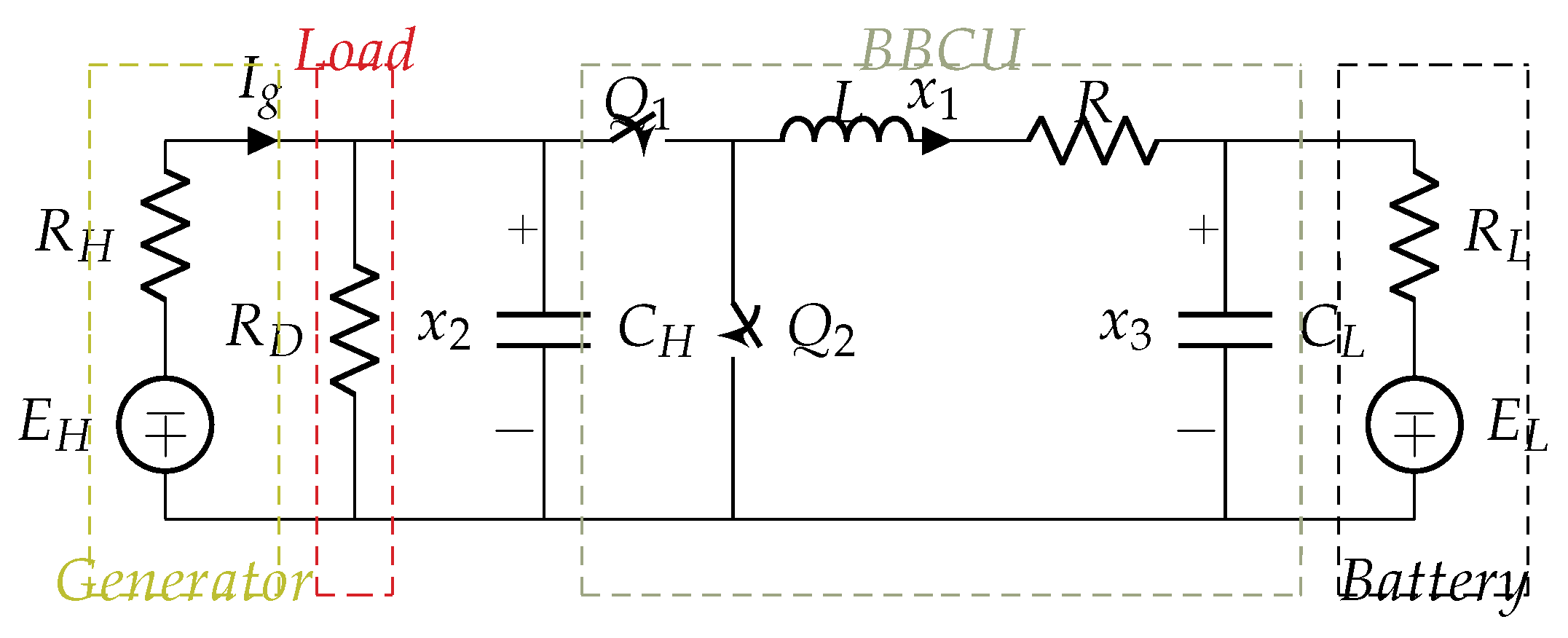
The control of the BBCU follows the steps in [17]. A, low-level strategy is designed to track prescribed current references. A high-level policy has the objective to define the current references to fulfil the control objectives stated in the Introduction. In this section, we briefly recall the results in reference [17], to which the interested reader is referred for mathematical details. Both control objectives, namely inductor current regulation (for the objective of Mode M1) and generator current limitation (that is the objective of Mode M2) can be recast in the following framework. Assume that the only task of the control is to keep the following function (6) equal to zero.

$$\sigma (t,y,x_2)=k\left(t\right)x_2-y$$

(6)

where: $k\left(t\right)=k_0{e}^{-\gamma t}+k_1$ is an exponential function, with $\gamma >0$. Please note that by choosing $k\left(0\right)=k_0+k_1=y\left(0\right)/x_2\left(0\right)$, the control objective $\sigma =0$ is achieved since the initial instant, so there will be no initial transient phase (“reaching phase” [24]) for zeroing $\sigma$. The sliding manifold-based controller used to keep $\sigma$ to zero at any time instant is

$$u\left(t\right)=\frac{1}{ϵ}\left(\sigma (t,y,x_2)+c{\int }_0^t\sigma (\tau ,y,x_2)d\tau \right)$$

(7)

with c and $ϵ$ are positive constants. The structure of the controller is simply a high gain Proportional-Integral (PI) control. However, with respect to classic PI’s, there are some peculiar characteristics of the proposed control. First, the variable that is fed back is not the classical tracking error, but the sliding function, which is the true novelty of the proposed approach. Second, there is no need for empirical tuning of parameters. Third, stability is rigorously proved without resorting to local linearization and the robustness is guaranteed by the theory of high gain control. Moreover, it is possible to prove that the system resulting from this control is linear and globally exponentially stable. This characteristic is very important, since for any mode the Region of Attraction becomes the whole space state. It is important to point out that this important feature is the result of the specific choice of the sliding Function (6). Then, to assess stability of the supervisory system, only an estimate of the dwell time will be needed.

Then, to fulfil control objectives required by Modes M1 and M2, the steady-state values for the inductor current and the capacitor voltages, say $(X_{1\infty },X_{2\infty },X_{3\infty })$, are computed analytically, as a function of the network and converter parameters. Next, the implicit algebraic equation

$$k_1{X}_{2\infty }=X_{1\infty }$$

(8)

is solved for $k_1$. Specifically, in Mode M1 $X_{1\infty }$ is given a desired value $X_{1\infty }=\overline{y}$ and $k_1$ is computed from Equation (8). On the other hand, when in Mode M2, note that the generator current can be written as

$$I_g=\frac{E_H-x_2}{R_H}.$$

(9)

It is clear that a fixed value of $I_g=I_{gM}$ can be imposed by assigning a fixed steady-state value for ${\overline{x}}_2=X_{2\infty }$, i.e.,

$${\overline{x}}_2=E_H-R_H{I}_{gM}$$

(10)

and solving again Equation (8) for $k_1$.

3.1. Theoretical Limitations on Setpoints

As mentioned above, from the explicit solution of Equation (8) it is possible to deduce the analytic expression for $k_1$. This analytic expression is useful to deduce theoretical bounds on the allowable setpoints that the controller can be asked to track.

For Mode M1, $k_1$ is given by [17]

$$k_1=\frac{E_H-\sqrt{E_H^2-4\left(\frac{R_H}{R_D}+1\right)[E_L+(R_L+R)\overline{y}]R_H\overline{y}}}{2R_H[E_L+(R_L+R)\overline{y}]}.$$

(11)

It is easy to prove that non-negativity of the term under square root implies the following key limitation on the current that the converter can track

$$-\frac{E_{LH}^{*}+E_L}{2(R_L+R)}\le \overline{y}\le \frac{E_{LH}^{*}-E_L}{2(R_L+R)}$$

(12)

where $E_{LH}^{*}=\sqrt{E_L^2+\frac{R_D}{R_D+R_H}\frac{R+R_L}{R_H}{E}_H^2}>E_L$.

Please note that when $R_D\to 0$, the maximum positive current reference approaches zero, and this has a clear physical meaning. Indeed, in this case, ever-increasing loads are added in parallel, the generator can only supply the load and has no power left for the battery. Conversely, when $R_D\to \infty$, i.e., the loads are absent, the maximum positive value of the current through the inductor is

$${\overline{y}}_{max}=\frac{\sqrt{E_L^2+\frac{R_L+R}{R_H}{E}_H^2}-E_L}{2(R_L+R)}.$$

(13)

In all the cases, it is clear that there is a limitation on the reference currents.

For the generator current limitation, i.e., Mode M2, solving Equation (8) for $k_1$, and replacing $X_{1\infty }=k_1{\overline{x}}_2$ results in

$$k_1=\frac{-E_L+\sqrt{E_L^2-4{\overline{x}}_2\frac{R+R_L}{R_H}\left[\left(1+\frac{R_H}{R_D}\right){\overline{x}}_2-E_H\right]}}{2(R+R_L){\overline{x}}_2}$$

(14)

also, in this case, for $k_1$ to be real, the following condition must be fulfilled

$$0<{\overline{x}}_2\le \frac{E_H+\sqrt{E_H^2+\frac{R_H}{R+R_L}(1+{\rho }_{HD})E_L^2}}{2(1+{\rho }_{HD})}$$

(15)

where ${\rho }_{HD}=R_H/R_D$ and the lower bound ${\overline{x}}_2>0$ is due to physical reasons. This in turn implies that the generator overload threshold is lower bounded by

$$I_{gM}>\frac{E_H}{2R_H}\left(1-\sqrt{\frac{1}{{(1+{\rho }_{HD})}^2}+\frac{R_H{(E_L/E_H)}^2}{(R_L+R)(1+{\rho }_{HD})}}\right)$$

(16)

3.2. Theoretical Limitations on Control

Another consideration is made in this section. The control law Equation (7) is a continuous control action, while it is clear that its practical implementation can be done only through switching, on/off devices. This can be done based on a theoretical result [37] stating that if the so-called equivalent control $u_0$ is in the interval $[0,1]$, then a switching, discontinuous implementation is possible retaining all the properties of the sliding mode approach (robustness, accuracy).

In reference [17], the equivalent control has been computed as

$$u_0\left(t\right)=\frac{L{C}_H}{(Lk{\left(t\right)}^2+C_H)x_{20}}\left\{\left[\dot{k}\left(t\right)+\left(\frac{R}{L}-\alpha \right)k\left(t\right)\right]x_{20}+\frac{x_{30}}{L}+{\beta }_{H}k\left(t\right)\right\}$$

(17)

Clearly, condition $0<u_0<1$ depends in a strongly non-linear fashion on the parameters, hence it is not easy to check it. Considering only the steady-state values, It is possible to plot the equivalent control as a function of the parameters to be selected. This is done in Figure 3 for the case of inductor current control, with the network and converter parameter values considered in Section 4. Please note that the equivalent control varies almost linearly with the desired current set-point, at least until the load resistance decreases too much (i.e., the load absorbs more and more power).

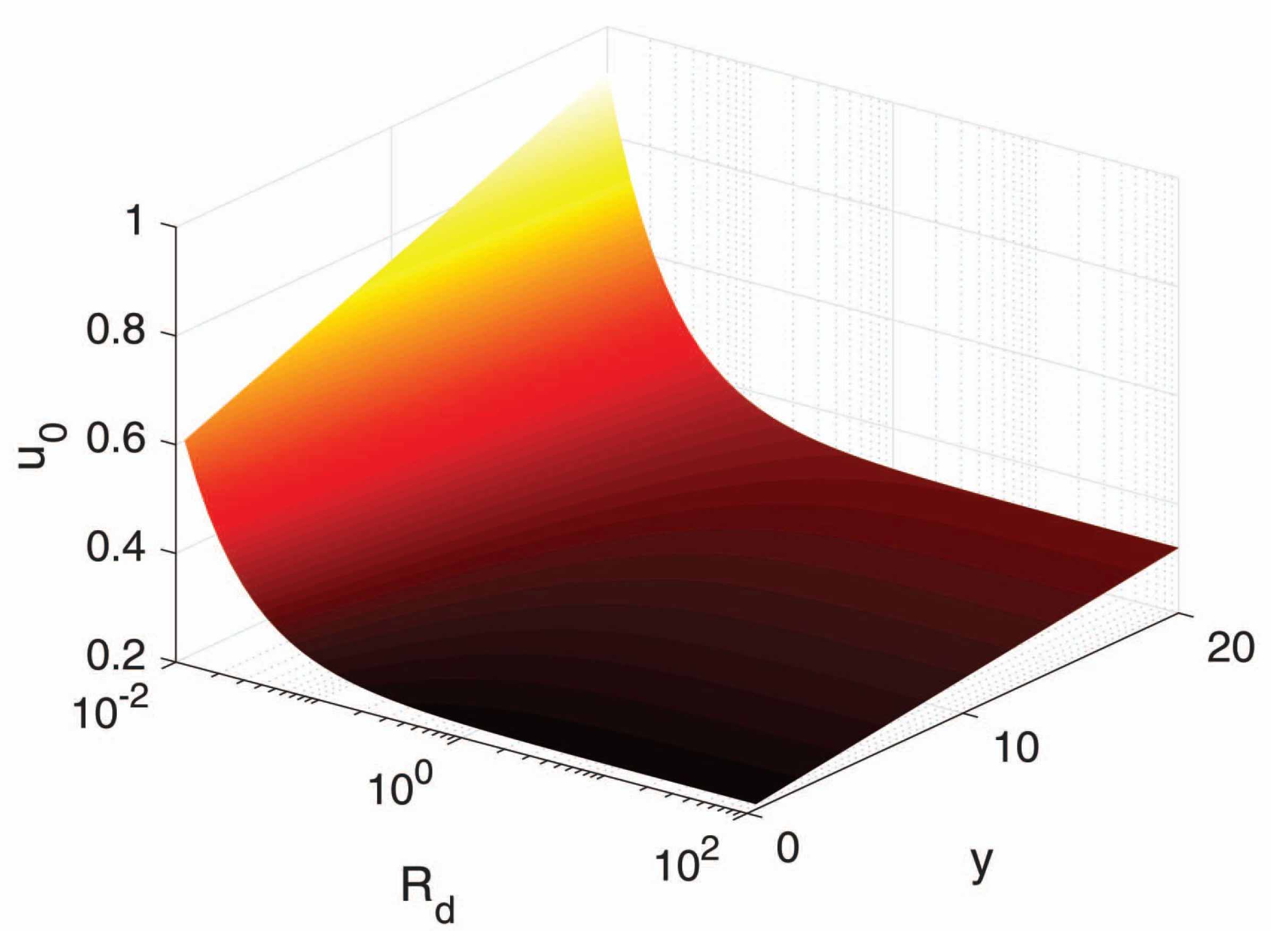
Analogously, when the objective is to alleviate generator overload, the general expression for $u_0$ at steady state as a function of the load resistance and of the maximum generator current can be computed and plotted, resulting in Figure 4.

In this case, the interpretation is more complex, but in any case for large load resistance the behavior is linear.

3.3. Machine Learning-Based Estimate of the Gain $k_1$

Although Equation (8) can be used to compute $k_1$, as discussed above in some practical implementations the analytic approach can be hardly viable. In this paper, we propose a different (and simpler) approach, able to counteract also uncertain knowledge of the converter and network parameter. Assuming that the load can assume only a finite set of values, it is possible, for any fixed load, to create a lookup table relating $k_1$, $\overline{y}$ and $I_{gM}$. This can be done directly on experimental set-up, thus overcoming problems due to poor component modeling or noisy measurements. The drawback is that a preliminary set of experiments must be carried out to set up the tables, and these experiments must be repeated for each value of load $R_D$. Obviously, this preliminary phase can be automatized: the simplest approach is to select $k_1$, perform the experiment with the closed-loop control Equation (7) and wait until the steady state is reached, then storing a filtered version of y and $I_g$. Then repeat with $k_1$ varying in a given interval. Remember that for any fixed $k_1$ the closed-loop system is stable due to the sliding manifold theory, so the experiments can be performed without worrying about stability issues, as should be the case with standard PI controllers.

The result is one table for each load, each as in the one shown in

Table 1. Table of Values for $R_D$ = 40 $\mathrm{\Omega }$.

${\mathit{k}}_1$	$\overline{\mathit{y}}$	${\mathit{I}}_{\mathit{gM}}$
$-0.040$	$-5.42$	5.09
$-0.030$	$-4.06$	3.08
⋮	⋮	⋮
0.025	3.39	6.99

, related to the case $R_D=40\mathrm{\Omega }$.

If we perform and “inversion” of the tables we can in principle also estimate the current value of the load from the measures of $k_1$, y and $I_g$. In other words, the values in Table 1 define for each $R_D$ a function ${\varphi }_{R_D}:\mathbb{R}\to {\mathbb{R}}^2$, $\overline{y},I_{gM})={\varphi }_{R_D}\left(k_1\right)$. Inverting this function means to compute a function ${\varphi }_{R_D}^{-1}$ such that $k_1={\varphi }_{R_D}^{-1}(\overline{y},I_{gM})$. Please note that this operation also requires an estimate of the load $R_D$, since the values in Table 1 are obtained with a fixed value of $R_D$. 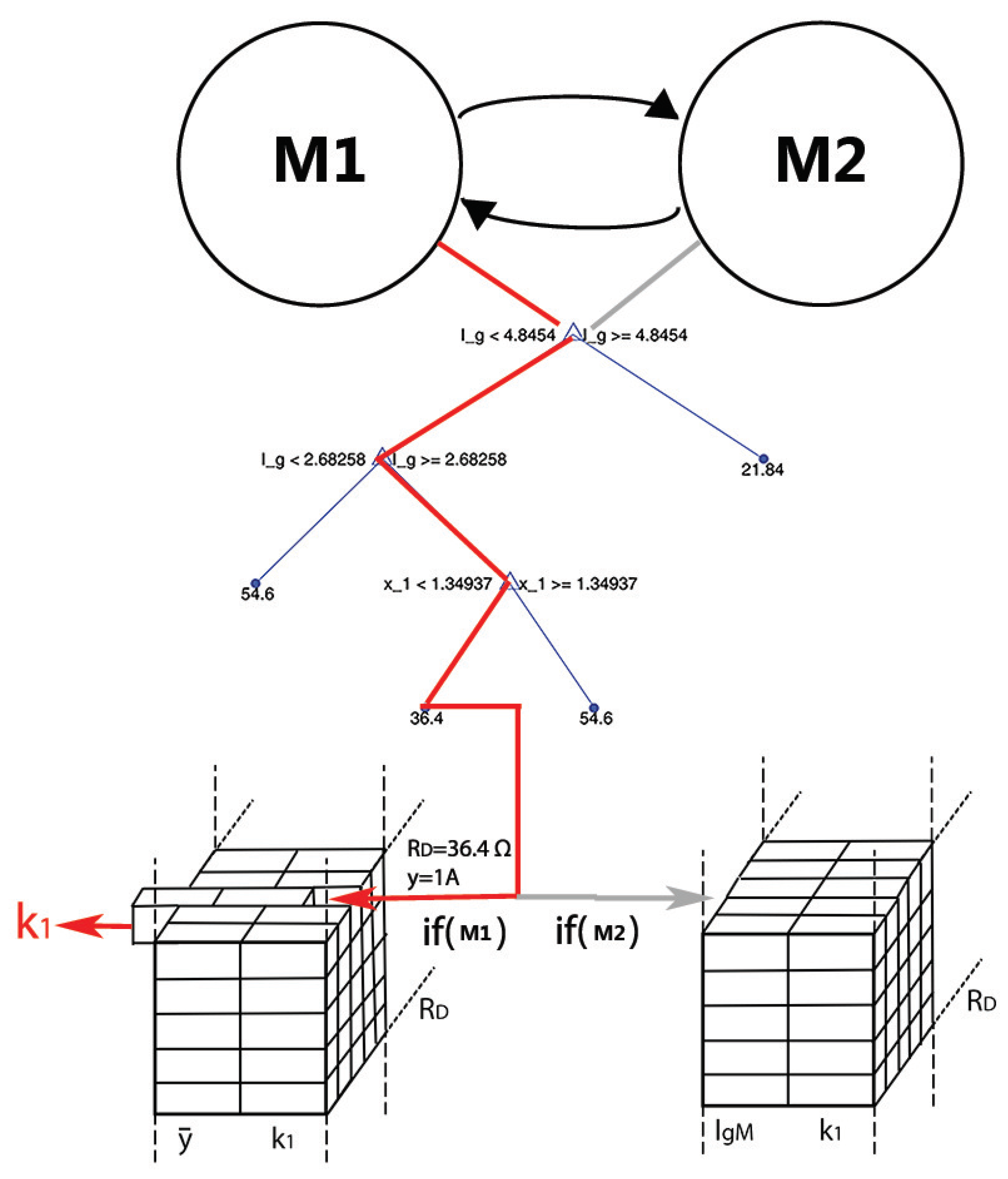This operation is usually non-linear and can be performed by resorting to supervised learning strategies, e.g., Support Vector Machine [38] or Decision Trees [39]. We have chosen the decision tree approach for its simplicity and easy interpretation of the results. The decision tree used in the application is depicted in Figure 5.

It has been obtained by training a decision tree [40] on the experimental data as follows. First, the decision variables have been selected, namely the generator and the inductor currents, then the values of load resistance have been considered as attributes. Finally, a binary decision tree has been fitted to the experimental data collected above. while on the leaves of the tree there are the values of the load resistance. More details on this approach are given in Section 5.

3.4. Design of Supervisory Control

In this section, the high-level controller defining the correct reference to follow is defined. As stated before, the objective of the supervisor is the intelligent management of the electric energy onboard the aircraft according to two operational Modes, M1 and M2, namely

• Constant inductor current (Mode M1)
• Constant generator current (Mode M2).

The crucial condition that imposes the commutation between the two modes is the event of current overload on the generator. More complex strategies are possible, e.g., when the battery is charged it can be used to reduce the generator load, or definition of different priorities on the loads, resulting in different responses to power request, but this topic will not be addressed here.

From a practical point of view, an implementation with a strict threshold would result in chattering behavior close to the threshold. For this reason, a hysteresis band is introduced, $[I_{gM}-\theta ,I_{gM}+\theta ]$ such that is the generator current exceeds the upper limit the supervisor enters Mode M2 and returns to M1 only if the generator current goes below the lower limit.

Please note that in both modes the load may change, and the controller must react to the change. This problem has been discussed in reference [17], and the reader is referred to this reference for detailed treatment. In synthesis, since the controller is switching among different stable configurations, to prove the stability of the overall strategy it is sufficient to assume that a minimum dwell time occurs between two consecutive commutations. In practical applications this means that the load is not allowed to vary randomly and very frequently, which is a reasonable requirement.

The structure of the supervisor is very simple and is shown in Figure 6. It consists simply of two nodes each for each mode (M1,M2). Please note that within each node the value of $k_1$ must be computed and possibly updated if the load changes.

The whole procedure can be summarized in the following steps.

• Set-up

  (a)

  Perform a set of experiments with different loads and save the results in different tables (one for each load) as in Table 1.

  (b)

  Compute the decision tree for the estimate of the loads, using $k_1$, $\overline{y}$ and $I_g$ as predictors and the loads as categorical labels.

• Runtime

  (a)

  Estimate the load by using the current values for $k_1$, y and $I_g$. Then using the table corresponding at the estimated load,

  (b)

  if in Mode M1, update, if needed, $k_1$ by looking at the column corresponding to the desired inductor current $\overline{y}$,

  (c)

  otherwise, if in M2, update $k_1$ by looking at the column corresponding to the desired generator current $I_{gM}$.

The points (2b) and (2c) detail the “$k_1$ computation” in Figure 6.

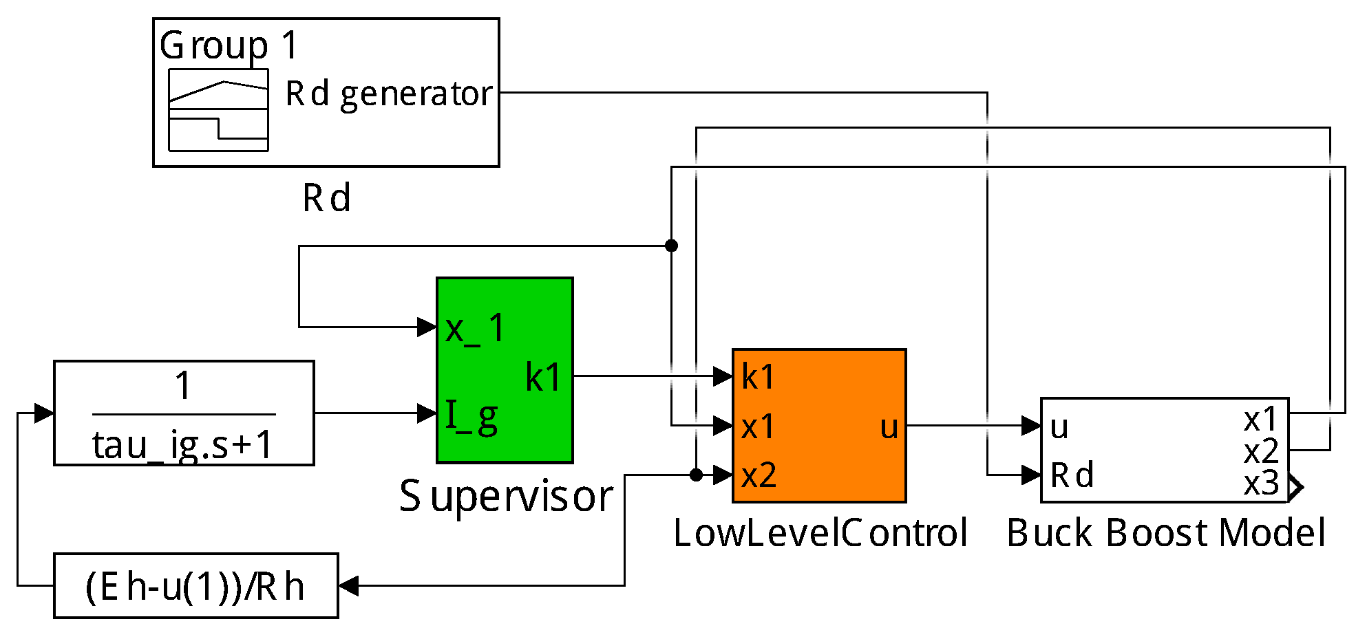
4. Simulation Results

To test the proposed strategy, first a simplified MATLAB/Simulink simulator (ver. 2016, The MathWorks, Inc, Natick, MA, USA) has been implemented as shown in Figure 7. The simulator is simplified since it does not consider switching elements, bus simply the model (1)–(4).

The load $R_D$ is variable and it is designed as a bank of two parallel passive components, i.e., resistors, which can be singularly connected to have a total load whose resistance is either one of the two or the parallels of them. The remaining parameters considered in the simulations are in

Table 2. System data.

$E_L$	28 (V)
$E_H$	135 (V)
L	0.9 (mH)
$C_H$	2.9 (mF)
$C_L$	2.6 (mF)
$R_H$	20 (m$\mathrm{\Omega }$)
$R_L$	37 (m$\mathrm{\Omega }$)
R	39 (m$\mathrm{\Omega }$)
$R_{D1}$	40 ($\mathrm{\Omega }$)
$R_{D2}$	60 ($\mathrm{\Omega }$)

. Please note that the high voltage (HV) bus voltage is half the standard 270 V value, while the LV bus voltage is the standard 28 V [41]. This is essentially due to hardware equipment limitations and does to affect the effectiveness of the results. Battery parameters are selected based on the following considerations. Considering a battery with four parallel stacks of 9 series connected cells each, with the standard cell voltage $3.2$ V, LiFePO${}_4$ battery [42], a reasonable model of a 28 V, (40 Ah) requires a stack total resistance $R_L$ indicated in Table 2.

The controller parameters are shown in

Table 3. Controller Parameter.

c	10
$\gamma$	10
$ϵ$	10
$\theta$	0.17
$I_{gM}$	5.9 (A)
$\overline{y}$	1.35 (A)

.

Please note that, although the control strategy is based on a high-gain approach, the realistic implementation through PWM with relatively low switching frequency (see Section 5) prevents the control designer from using high gains. Obviously, the price to pay is a reduced accuracy regarding the high gain implementation.

Moreover, the measured current of generator $I_g$ is filtered by the filter

$$G\left(s\right)=\frac{1}{{\tau }_{g}s+1}$$

(18)

with ${\tau }_g=0.01$ s. The filtered generator signal is used simply to detect the occurrence of an overload.

The supervisor is implemented in State Flow with two states only, as shown before.

The system can be in two states:

• $M1$, in which the goal is to drive $x_1$ to the reference $\overline{y}$;
• $M2$, in which the goal is to drive $I_g$ to the reference $I_{gM}$.

The computation of $k_1$ is performed by using different lookup tables, as stated in Section 3.3. Specifically, starting from the data in tables such as Table 1, one table for each load, we define a 3D array in each mode: in M1 the array has different values of $x_1$ and $k_1$ for each load $R_D$, while in M2 the values for $I_g$ and $k_1$ are stored, for the different loads.

The overall procedure goes as follows. First, the generator current is estimated through the Filter (18), and the current mode (M1 or M2) is defined. Next the current load is estimated through the decision tree. Please note that the true value of the actual load is irrelevant, since the decision tree treats the load as a categorical value. Next, the algorithm extract from the 3D array the table related to the computed value of load $R_D$. Finally, a lookup table search yields the value of $k_1$ to be used in the control law. For example, in Figure 8, assuming that the generator is supplying $I_g=3$A, while the current through the inductor is $y=1$A. Then the supervisor is in state M1, the first 3D array is selected and the decision tree computes $k_1=0.01$. Incidentally, note that the decision tree estimates the load as $R_D=36.4\mathrm{\Omega }$.

As stated in Section 3.4 a minimum dwell time [43] must be guaranteed before a load change is allowed. The approach presented in [17] is based on the idea that a new commutation is allowed only when the total energy has decreased at least to the value it had before the commutation, so that no net increase of energy is possible.

With the values in Table 2 and Table 3, a rough estimate of the dwell time ${\tau }_{\delta }$, based only on the maximum and minimum load is given by ${\tau }_{\delta }=0.2$ s. Therefore, assuming that consecutive load variations do not happen before the time ${\tau }_{\delta }$ has elapsed, the controlled system is guaranteed to be stable.

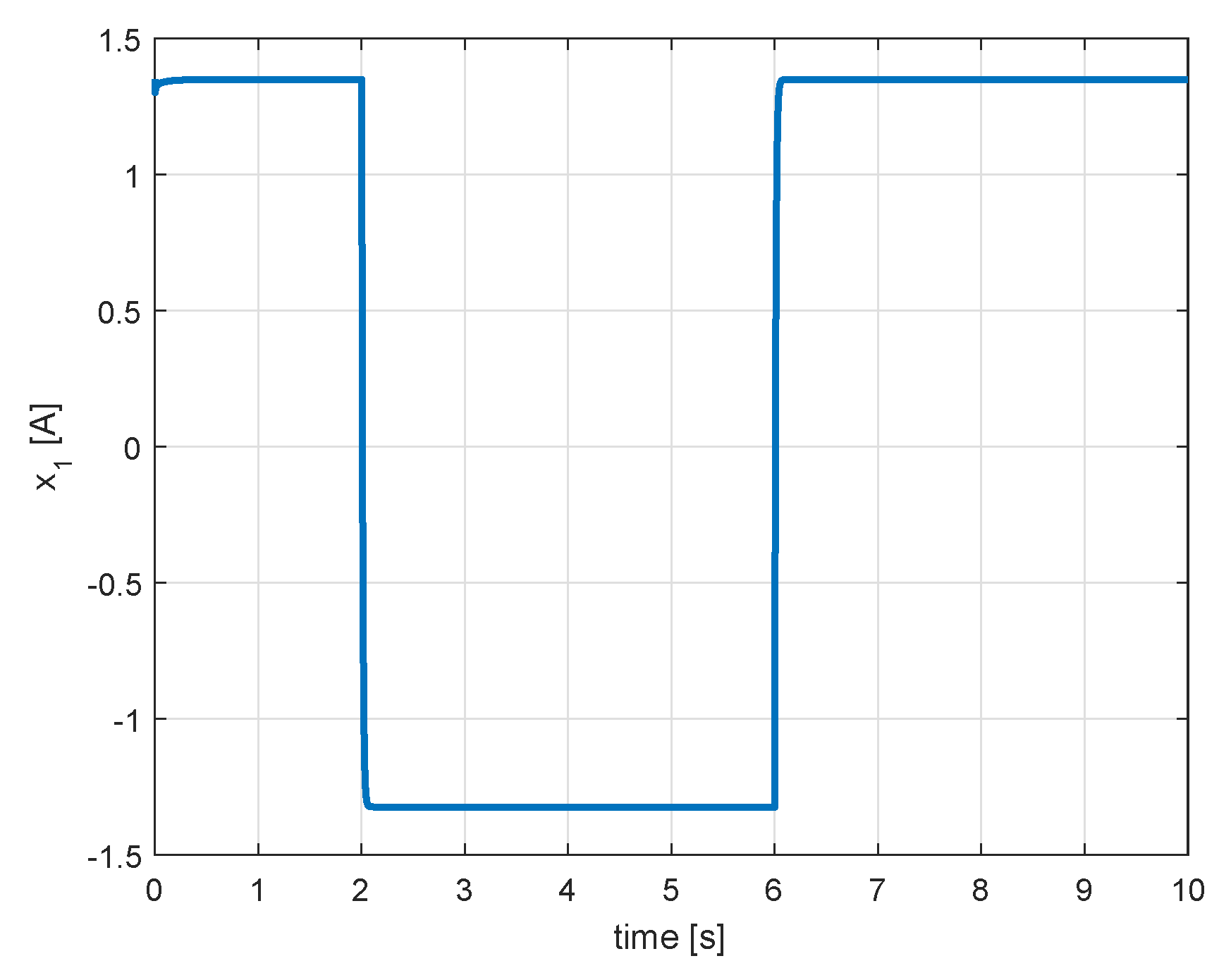
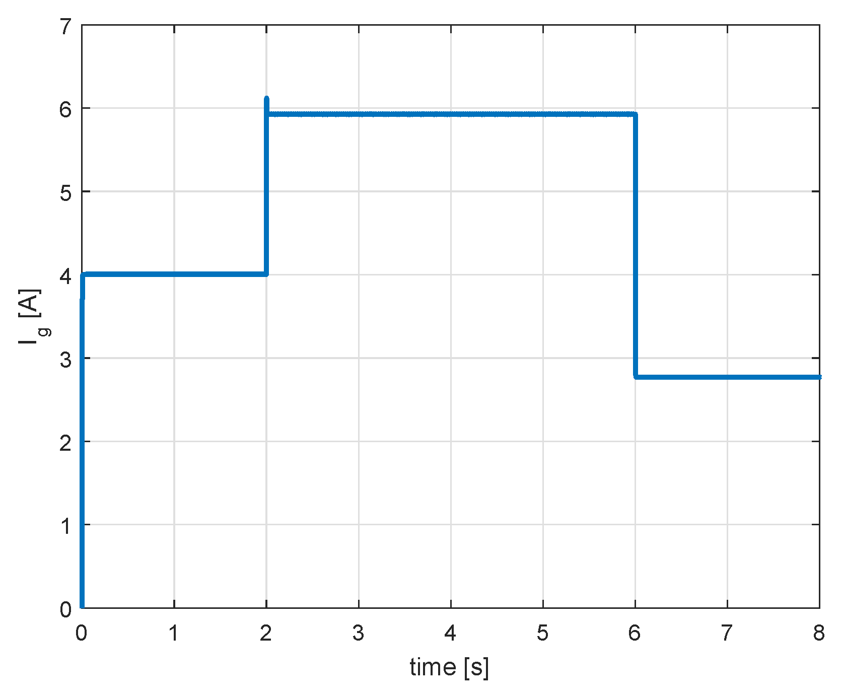
The simulation consists in three phases. In the first one the system starts with load $R_D=R_{D1}$, where the generator current is less than the overload current, so it stays in the Mode M1, in which the inductor current follows the reference $\overline{y}$. In this stage the battery is recharged. Figure 9 shows that the current $x_1$ is driven quickly to $1.35$A, whereas Figure 10 shows that $I_g$ is not in overload.

At time instant $t=2$s a new load is added and now the total load of the system is the parallel between $R_{D1}$ and $R_{D2}$. In this phase, the generator current is in overload, so the supervisor switches to Mode M2, and the goal is to drive $I_g$ to $I_{gM}$. This is apparent in Figure 10. Please note that the flux of energy changes its sign, i.e., the inductor current becomes negative and the battery helps the generator to supply the load (Figure 9). Finally, at time $t=6$s the load $R_{D1}$ is removed, and so the overload vanishes, bringing the system again in Mode M1 (but with load $R_D=R_{D2}$, different from the first situation) and the inductor current follows the imposed reference $\overline{y}$. As far as the control is concerned, Figure 11 shows that equivalent control is correctly in the range $[0,1]$. An important comment must be done on the robustness to uncertain parameters. Although the exact values of parameters are obviously unknown, as will see in Section 5, the control is effective both in simulation and in experiment. This is due to the robust control strategy, which absorbs the uncertainties.

Next, to test the effectiveness of the control system, a more detailed simulator has been designed, before the final experimental results. Specifically, a more complex model has been implemented by using the PowerSystems blockset in MATLAB/Simulink. The model considers physical models of the electric/electronic components and switching implementation of the power stage by means of a PWM with fixed frequency. This simulation has been set up to “bridge the gap” between simulation based on mathematical modeling and experiments. The scheme is in Figure 12. Figure 13 and Figure 14 show the results. Note the presence of chattering due to PWM switching. The average value of the control is shown in Figure 15.

Finally, for the proposed multi-objective supervisory control to be applicable, compliance with the most used aeronautical standards should be checked. In particular, MIL-STD-704F [41] prescribes, for DC bus, certain limits for transient and steady-state voltage, as reported in Figure 16.

Referring to Figure 16, for a nominal value 270 V, as a transient event happens the voltage can vary in the range $[200,330]$ V for 10 ms, and then it must recover, within 30 ms a steady-state value in the range $[250,280]$ V. Since in our case we have used a scaled version of the nominal voltage (i.e., 135 V that is just half the MIL standard voltage), it is sensible to consider a scaled (i.e., halved) version of the requirement, thus asking for the voltage to remain within $[100,165]$ V during the transient and $[125,140]$ V at steady state. As it is apparent from Figure 17 the requirement is largely satisfied by the proposed control law, since even during the transient the most stringent steady-state requirements are fulfilled.

5. Experiment Results

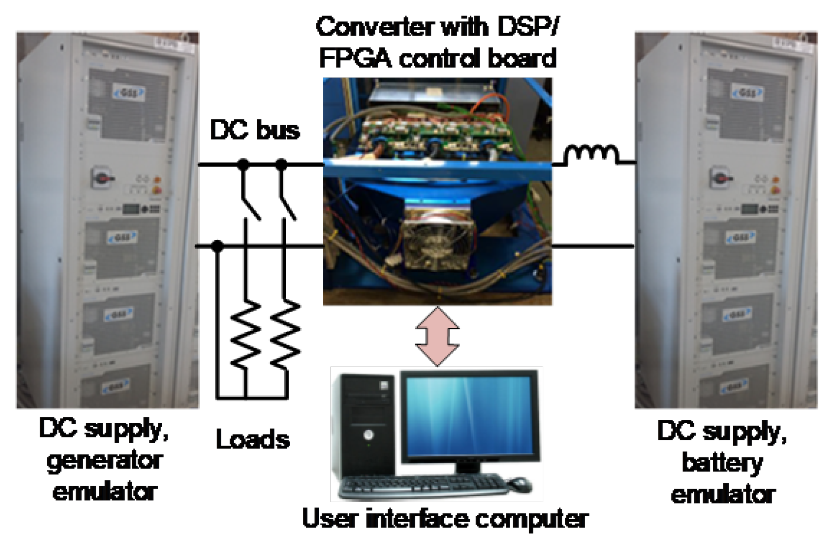
We have used a previously built laboratory DC/DC converter based on Insulated Gate Bipolar Transistor (IGBT) modules with low switching frequency (16 kHz) and large deadtime (1.5 $\mathsf{\mu }$s) in order to reduce the effect of the large deadtime on the accuracy of the results. We have chosen these specific voltage levels to guarantee operation at a relatively high value of the duty cycle to offset the effect of large deadtime and such low switching frequency.

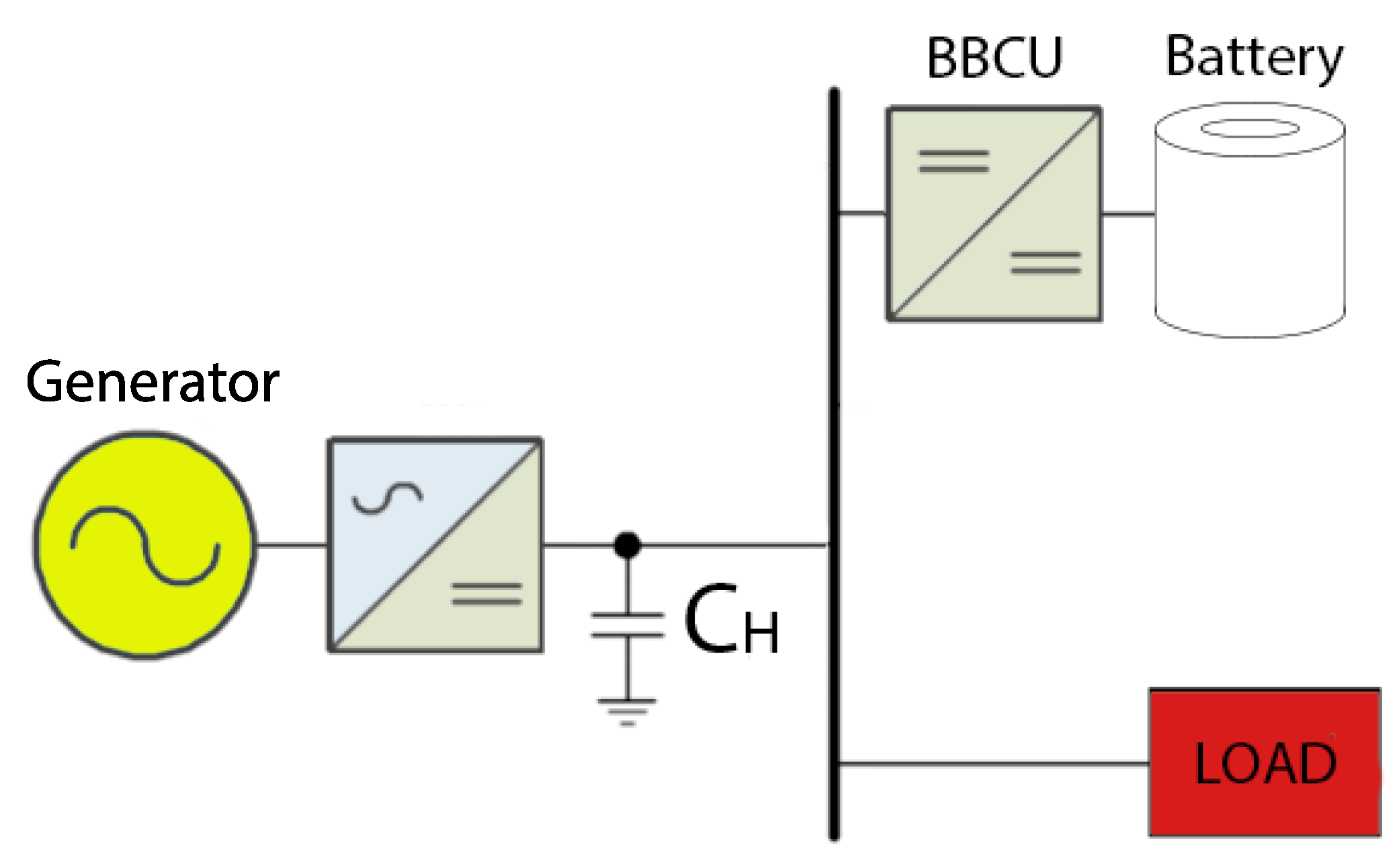
The laboratory set-up to implement the power system topology and to test the effectiveness of the proposed control and the EM management strategy is schematically shown in Figure 1. The block diagram of the laboratory set-up is shown in Figure 18, where two bidirectional DC power supplies are used to emulate the generator and the battery characteristics and behavior. The two DC power supplies used are of TC.GSS series from REGATRON (Programmable Grid-tied Source/Sink, Plattsburgh, NY, USA), which is a full bidirectional series of high-power DC source/sink units with internal novel bidirectional converter architecture allows for very fast and continuous “quadrant crossing” between source and sink operation and vice versa. The TC.GSS series is fully programmable and can be easily programmed by the user to mimic different types of electrical sources and loads such as batteries and generators with specific voltage droop characteristics. The battery emulator DC supply is interfaced to the DC bus by a DC/DC converter controlled by a DSP/FPGA control board (C6713 DSP STARTER KIT, Farnell, Stafford, TX, USA).

The DC bus is connected to the generator emulator DC supply and two resistor banks are connected to the DC bus by two contactors to mimic the power system loads.

The parameters of the system components are set according to the BBCU data shown in Table 2. The equivalent parameters of the generator and the battery emulators are ($E_H$, $R_H$, $C_H$) and ($E_L$, $R_L$, $C_L$) respectively. The DC/DC converter is built using an IGBT module with two switching devices $Q_1$ and $Q_2$. The parameters of the battery interfacing inductor are L and R. The resistance of the two resistor banks emulating the loads are $R_{D1}$ and $R_{D2}$. The proposed control algorithm is implemented and executed by the DSP-FPGA control board and the switching and the sampling frequency were set to $16$kHz. The DSP-FPGA internal control signals are captured by an interface program run on the user interface computer, see Figure 18. The simulation validation test scenario with the results shown in Figure 13, Figure 14 and Figure 15 is also validated experimentally using the laboratory set-up shown in Figure 18. The corresponding experimental test results are shown in Figure 19, Figure 20 and Figure 21. 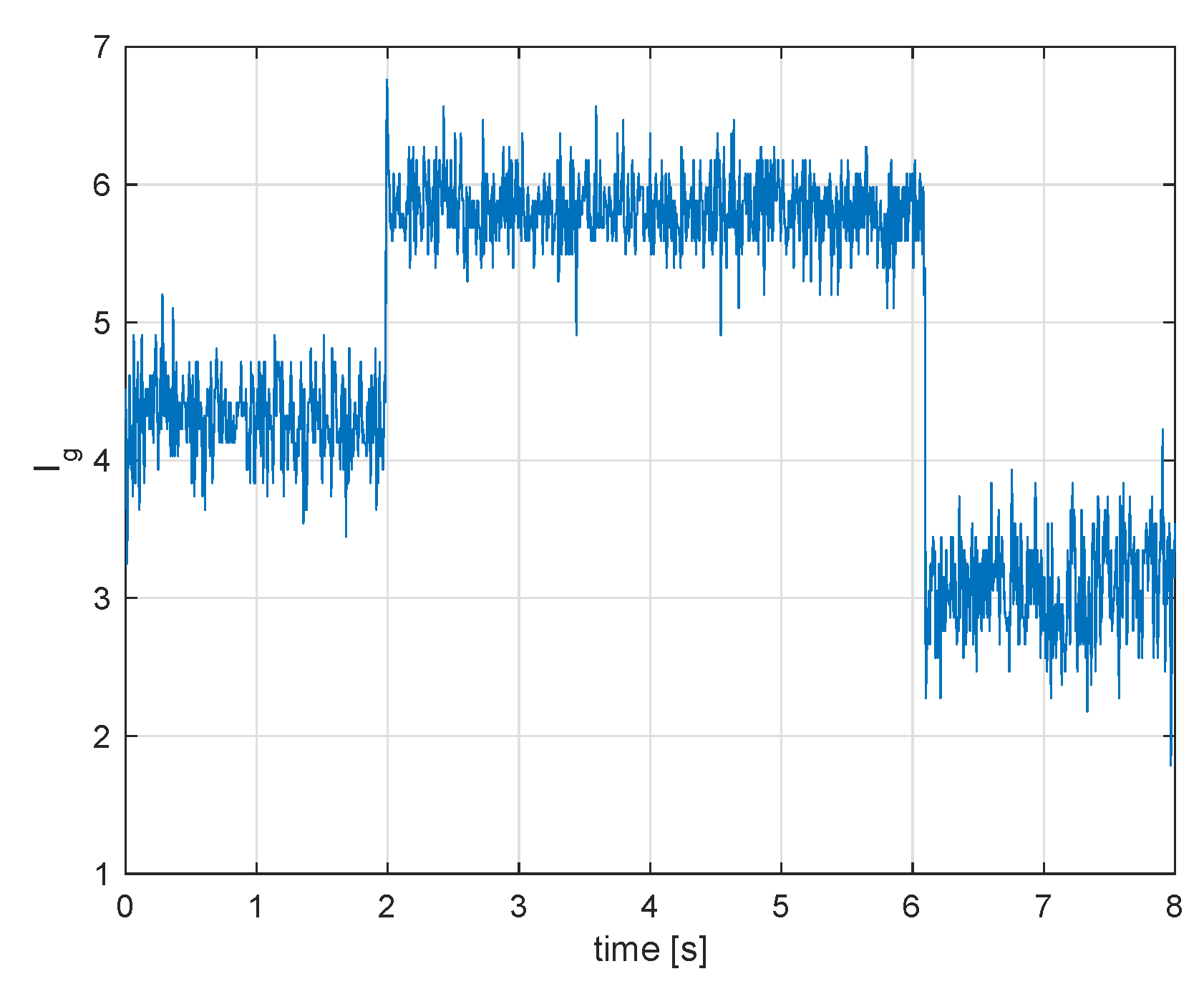Figure 19 and Figure 20 show the measured inductor and the generator current or the experimental test. It is noted that the inductor current shows a slower dynamic response compared to the simulation test results, which is due to unmodeled filtering and delay aspects of the experimental set-up. Also, the control condition $0<u<1$ is confirmed as shown in Figure 21. Although the noise to signal ratio of the experimental set-up signals is higher, the experimental results in general have demonstrated the effectiveness of the control algorithm and in are in good match with simulation results.

Finally, fulfilment of voltage limits is checked, as at the end of Section 4. Also, in this case, although the experimental values are noisier, the limits are largely fulfilled, as shown in Figure 22, where the HV bus voltage is shown along with its filtered version (to improve readability).

6. Conclusions

A supervisory control strategy has been presented for advanced MEA applications. In normal operations the battery is charged with an intermittent charging strategy, while in emergency cases, i.e., the occurrence of an overload, the goal becomes generator current limitation, so that the sizing (and the weight) of the generator can be reduced. This is done by exploiting the 5 s 5 min overload capability of the generator, and is thanks to the speed and robustness of controller. A two-level mathematically sound non-linear control strategy is considered. However, mathematical correctness should not result in complex implementation. A sensible way to show that the proposed strategy does not require extra complexity in the implementation is to apply it to a pre-existing test bench. This has been done in this paper, by considering a simple and relatively low-performance set-up (e.g., low-frequency switching converters, large deadtime), heavily based on off-the-shelf components. Functional and behavioral (detailed) simulations have been carried out to prove the concept and to compute the parameters of the controller. Next, an experimental campaign on the above experimental set-up has been performed to train a decision tree to estimate the current, unknown load. Finally, experiments have been carried out and compared with the expected results from the theory. The results match well and it is shown that both simulations and experimental results largely fulfil the specs (a reduced version of the MIL standard).