Hourly Day-Ahead Wind Power Prediction Using the Hybrid Model of Variational Model Decomposition and Long Short-Term Memory

Abstract

A more accurate hourly prediction of day-ahead wind power can effectively reduce the uncertainty of wind power integration and improve the competitiveness of wind power in power auction markets. However, due to the inherent stochastic and intermittent nature of wind energy, it is very difficult to sharply improve the multi-step wind power forecasting (WPF) accuracy. According to theory of direct and recursive multi-step prediction, this study firstly proposes the models of R (recursive)-VMD (variational model decomposition)-LSTM (long short-term memory) and D (direct)-VMD-LSTM for the hourly forecast of day-ahead wind power by using a combination of a novel and in-depth neural network forecasting model called LSTM and the variational model decomposition (VMD) technique. The data from these model tests were obtained from two real-world wind power series from a wind farm located in Henan, China. The experimental results show that LSTM can achieve more precise predictions than traditional neural networks, and that VMD has a good self-adaptive ability to remove the stochastic volatility and retain more adequate data information than empirical mode decomposition (EMD). Secondly, the R-VMD-LSTM and D-VMD-LSTM are comparatively studied to analyze the accuracy of each step. The results verify the effectiveness of the combination of the two models: The R-VMD-LSTM model provides a more accurate prediction at the beginning of a day, while the D-VMD-LSTM model provides a more accurate prediction at the end of a day.

1. Introduction

Wind energy is one of the fastest growing renewable energy sources in the world, representing an environmentally-friendly and rapidly developing wind power technology with renewable advantages [1]. Due to the influences of weather, environment, and power generation equipment on the output of wind power generation, its power curve has strong volatility and intermittency. When a certain threshold is exceeded, it has a great impact on the power quality and grid operation reliability after grid connection [2,3]. Therefore, it is of great practical significance to carry out more accurate forecasting in advance, so as to extend the forecasting step of wind power production, adjust the dispatching plan in time, reduce the operating cost of the power system, and determine the appropriate wind power price [4].

Wind power forecasts (WPFs) can be divided into four different types: very short-term (a few seconds to 30 min), short-term (30 min to 6 h), medium-term (6 h to 24 h), and long-term (one day and more) [5]. The China National Energy Bureau (NEB) enacted a regulation in 2011 that requires the hourly prediction of day-ahead WPFs for dispatching preparation. In addition, the maximum error of the daily forecast curve should not exceed 25%, and the root mean square error (RMSE) of the all-day forecast results should be less than 20% [6]. Due to the randomness of wind power output forecasts, wind power has brought new demands to the safe operation of the power system. Hence, day-ahead WPFs, especially for WPFs up to 1–24 h, have become a hot button issue in wind power systems and new energy domains with the implementation of large-scale wind power projects [7].

The mainstream WPF methods are generally divided into physical methods and machine learning methods [8]. Physical methods aim to describe the physical process of the transformation from wind power to electric energy, and physical models rely on numerical weather prediction (NWP) [9]. Since multiple parameters are involved in NWP, and wind farms are located in sparsely populated regions, complete data can be hardly guaranteed [10]. The statistical methods applied in the WPF field are mostly time-series-based approaches, and the future value of wind power can be expressed by a linear or nonlinear function of its historical data [11,12]. Instead, machine learning methods can characterize a nonlinear and complicated relationship of the networks—between input data and output data—and provide a WPF by applying various algorithms to this network. The artificial neural network (ANN), employing different structures such as feed-forward neural networks (FFNNs), extreme learning machines (ELMs), and support vector machines (SVMs), has been used to learn exemplar patterns of wind power. However, multi-step WPFs using statistical and machine learning methods have rarely been studied, because a greater number of forecasting steps corresponds to a lower accuracy. Specifically, the conventional shallow neural network (SNN) models often exhibit several shortcomings such as slow convergence and overfitting. Moreover, they are easy to trap into the local minimum when applied to high-dimensional and complex problems [13]. However, one effective way to address the shallow model issue is the use of deep learning, which has the ability to discover the inherent abstract features and hidden high-level invariant structures in data. The characteristics that are specific to feature extraction make deep learning much more attractive for WPF methods. In summary, the unsatisfactory feature mining of the shallow model and existing problems for individual forecasters inspires us to rethink the WPF problem based on deep learning architecture and the ensemble technique.

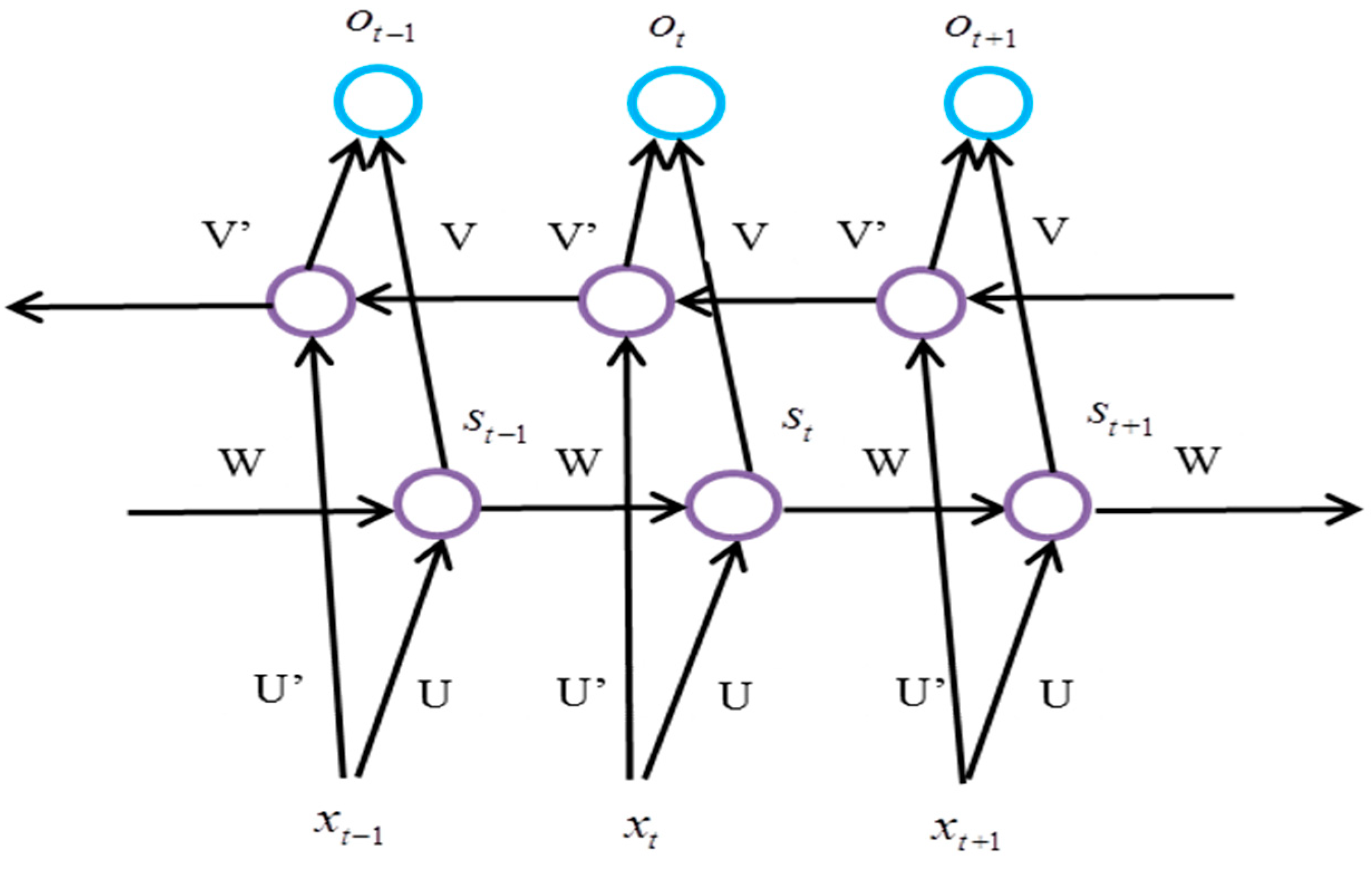
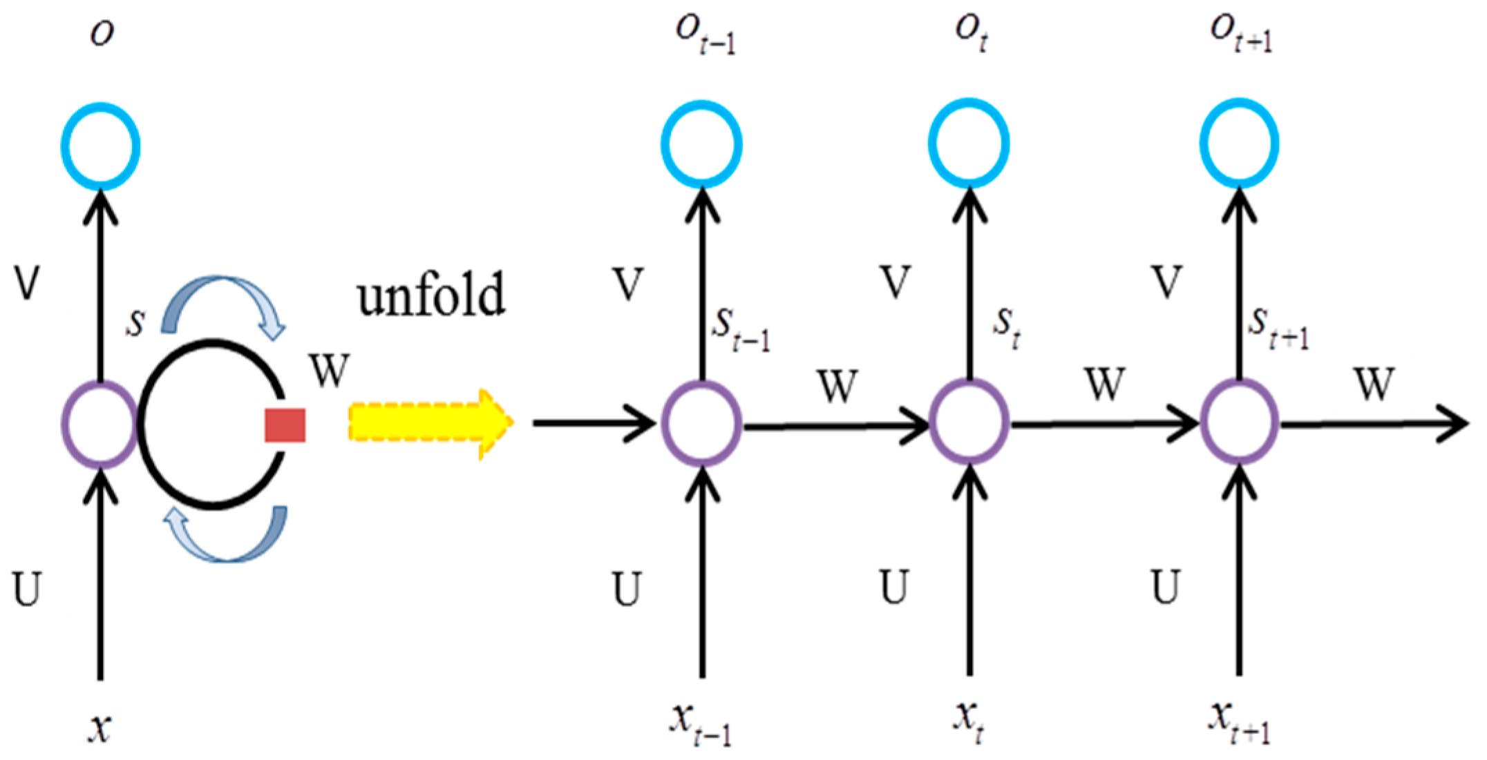
To address the shallow model issues, researchers have realized that the deep neural network (DNN), which contains the convolutional neural network (CNN), deep belief network (DBN), and recurrent neural network (RNN), can be applied to handle complex nonlinear relations and dynamics [14,15]. Unlike the traditional ANN, the RNN can discover the inherent abstract features and hidden high-level invariant structures in data. The characteristics that are specific to feature extraction make deep learning much more attractive for WPF methods. Specifically, the output of the RNN depends on previous computations as well as calculations of the current time step. However, due to the difficulty of learning long-range dependencies, the training of the RNN can be extremely challenging. 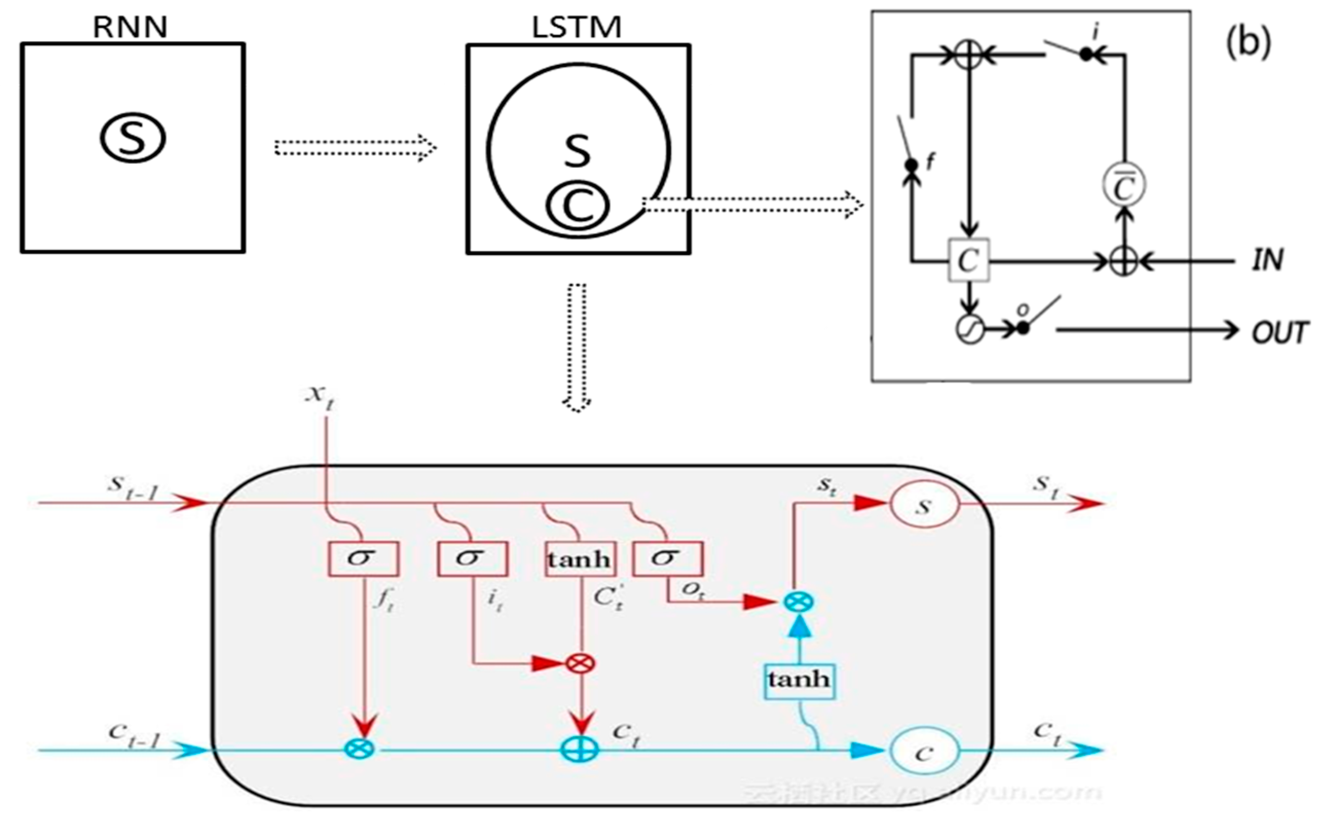This problem is commonly known as the vanishing/exploding gradient problem [16]. A previous work proposed a novel prediction model for recursive multi-step wind speed forecasting based on long short-term memory (LSTM). As a special RNN model, a LSTM network can avoid gradient vanishing and gradient explosion in the RNN training process to a great extent, thereby making full use of the large amounts of training data for classifying and forecasting as well as clustering analyses [17]. LSTM is an advanced approach in natural language processing, which considers not only the current word, but also other adjoining words in the sentence or even paragraph. Data with this kind of contextual information is called sequential data. Stimulated by the success of LSTM on machine translation, a few previous works have explored the power of LSTM on time-series prediction, and obtained promising results. For example, in reference [18], the authors Qu et al. employed principal component analysis (PCA) for data dimension reduction and established an LSTM-based short-term wind power prediction model. According to their results, the prediction accuracy of LSTM was significantly enhanced compared to the results of back propagation (BP, which is one of the training algorithms including multiple layers of perceptron) and support vector machine (SVM). In the literature [19], a wind speed prediction model was presented based on variational mode decomposition (VMD), singular spectrum analysis (SSA), an LSTM network, and extreme learning machine (ELM), in which the LSTM was employed as the predictor. Their work firstly proposed a novel prediction model for recursive small multi-step wind speed forecasting based on the LSTM, while our current study focuses on the direct and recursive forecasting model for wind power prediction of up to 24 steps.

In terms of prediction, pure statistical forecasts show that excellent performances under certain conditions are usually unavailable beyond 6 h [20,21]. Apart from these basic statistical methods, preprocessing methods such as time-series decomposition (TSD) also play important roles in forecasting. The multiple frequency components that always exist in a wind power series are considered the challenging parts in big multi-step forecasting. To address this problem, empirical mode decomposition (EMD) has been widely applied to decompose the original complex time series into several simply structured series, before the datasets are constructed and input into the basic predicting model [22]. The EMD method can divide the signal into several so-called Intrinsic Mode Function (IMF) components. Since the decomposition is based on the local characteristic time scale of the data, it can be applied to a non-stationary time series of produced wind power. 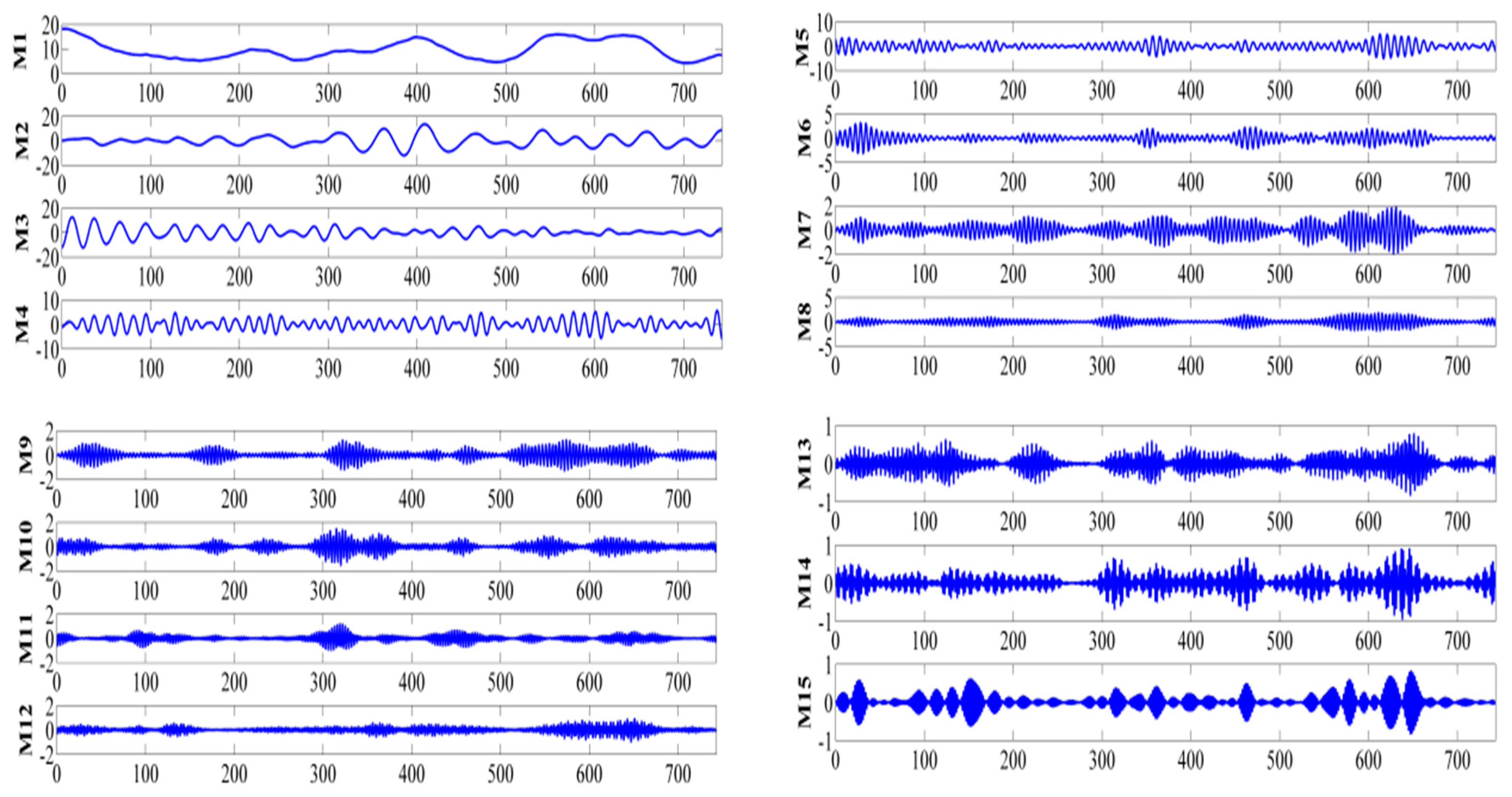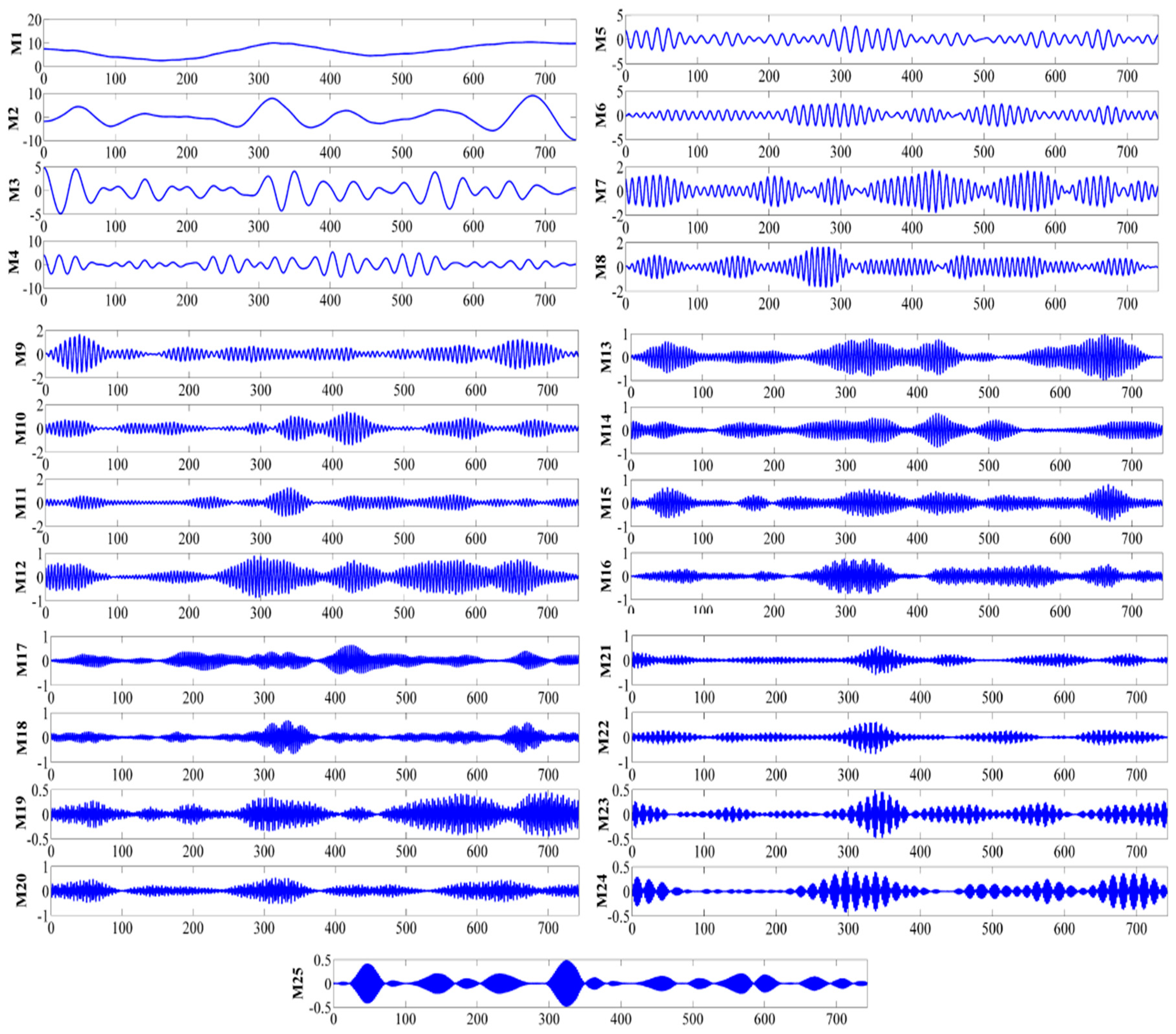The number of IMFs can be changed according to the harmonic content of signals, which has also been seen as the main disadvantage of EMD [23,24,25]. Based on the above-mentioned information, a decomposition method named variational model decomposition (VMD) was introduced for the purpose of improving big multi-step prediction accuracy for hourly day-ahead wind power generation. Unlike EMD, VMD transforms the signal into a non-recursive signal and has a good self-adaptive ability to remove the stochastic volatility [26].

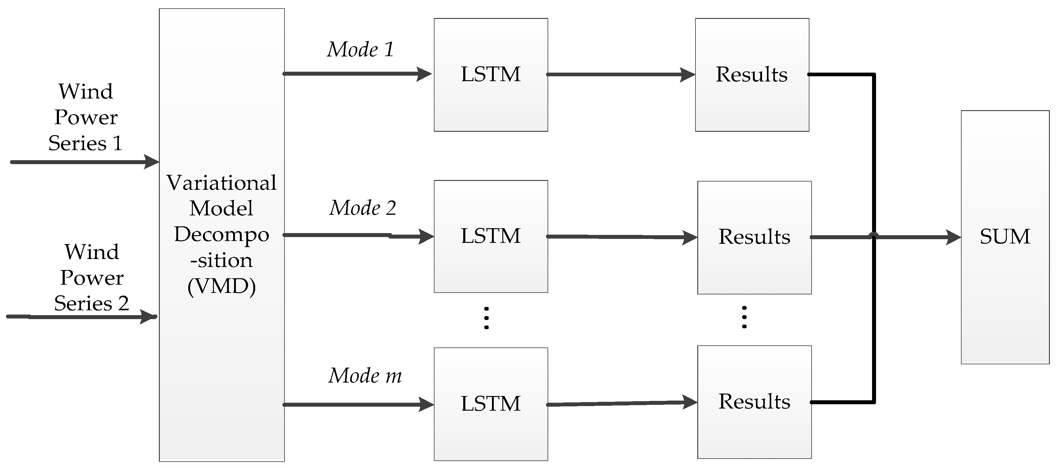
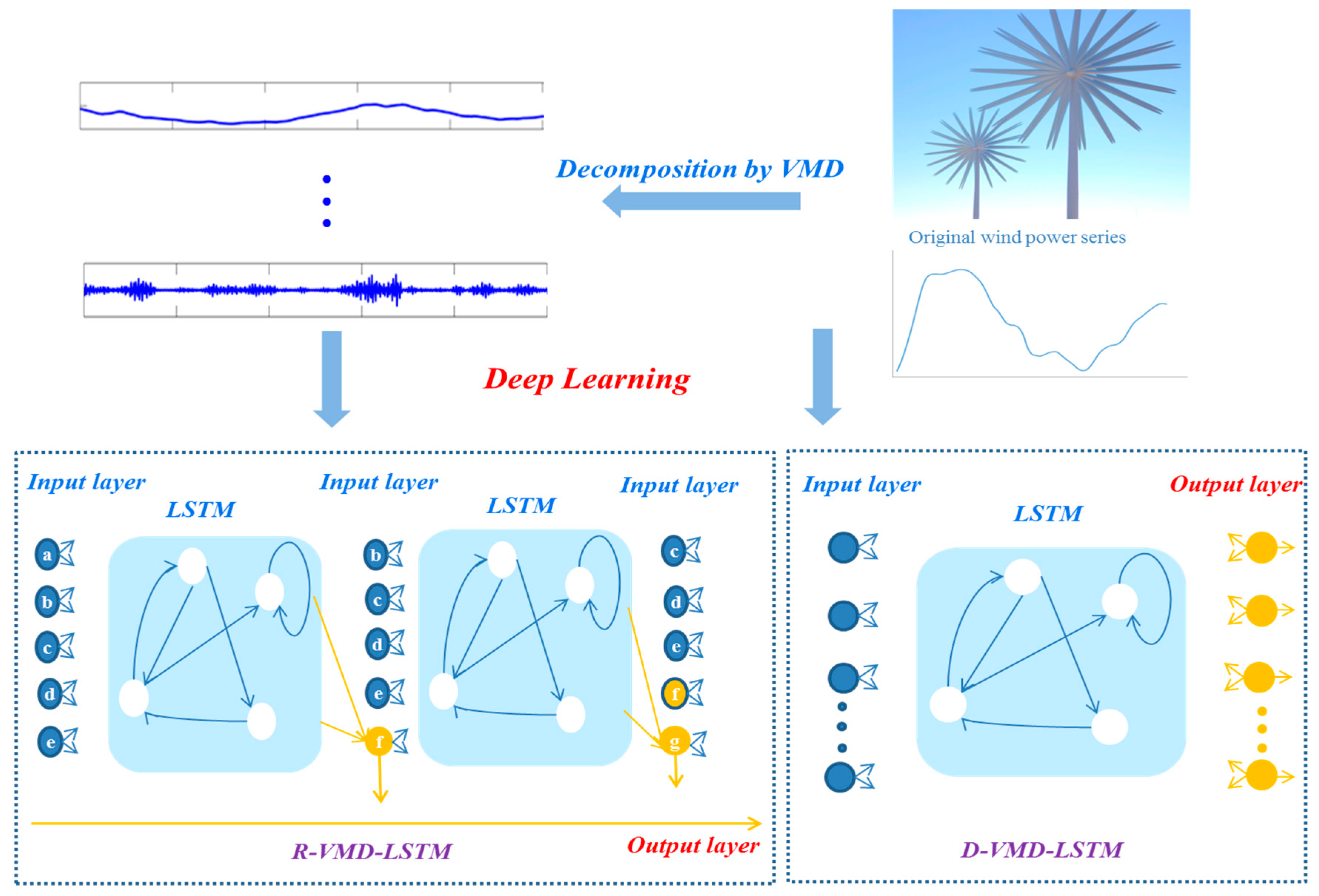
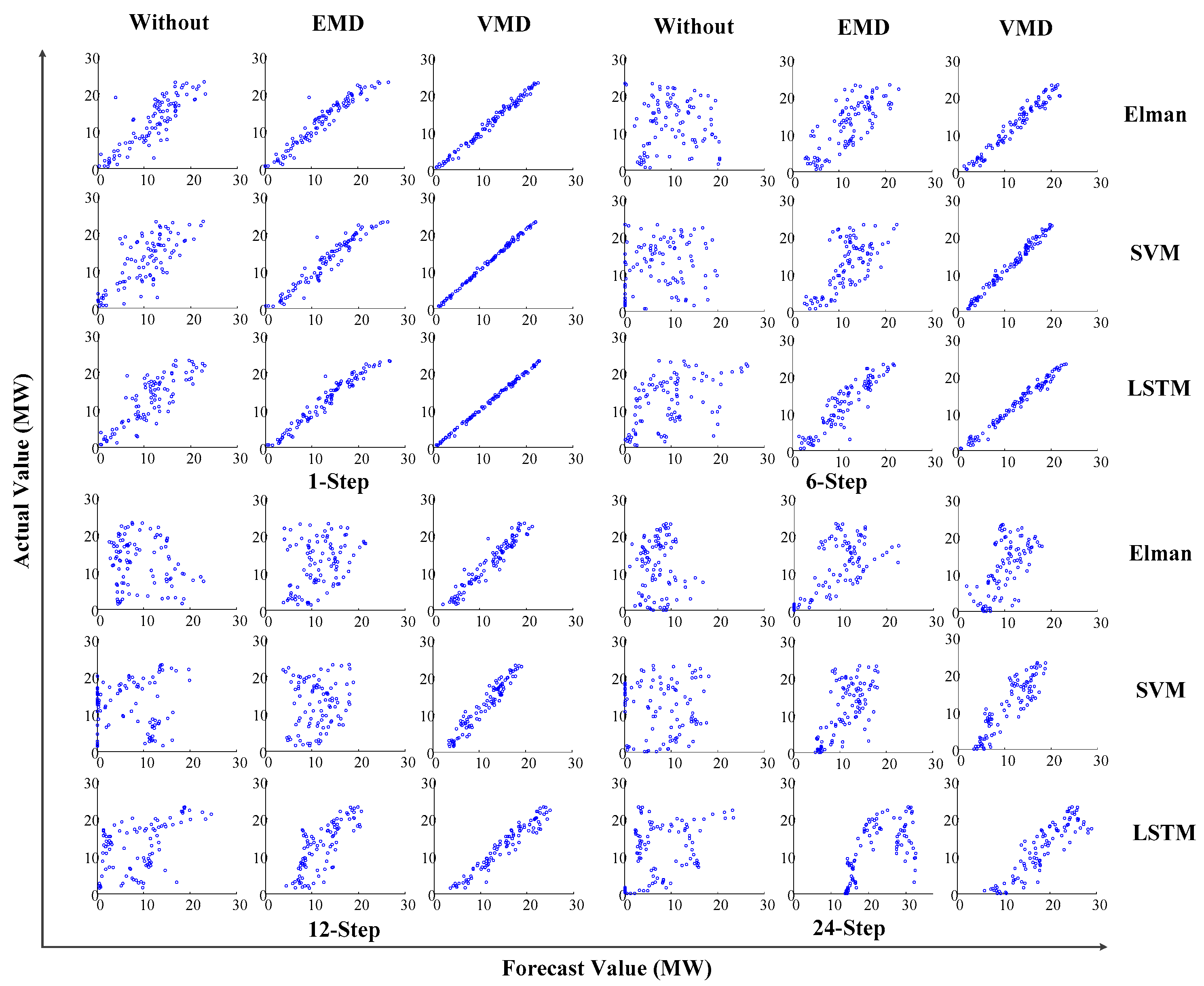
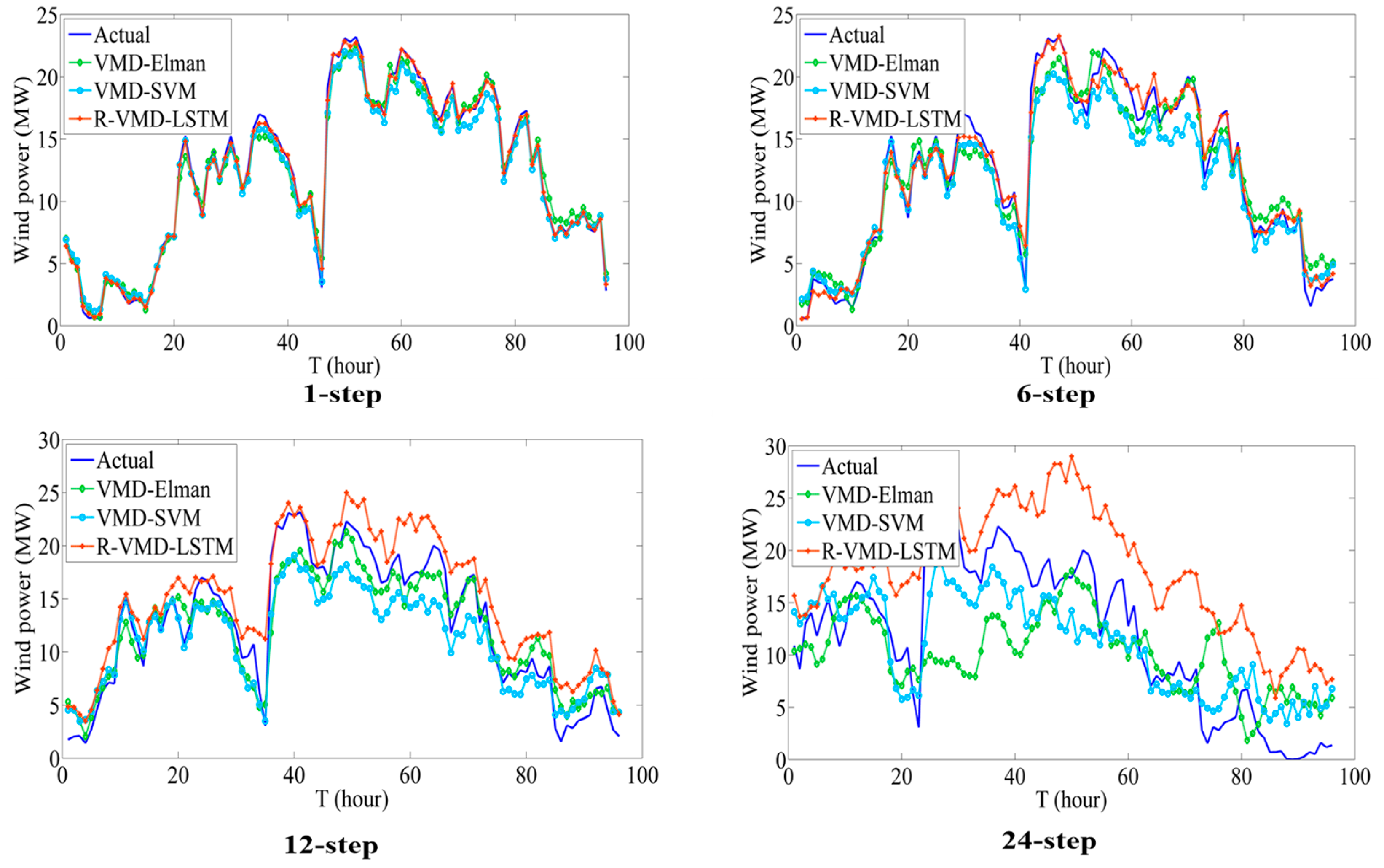
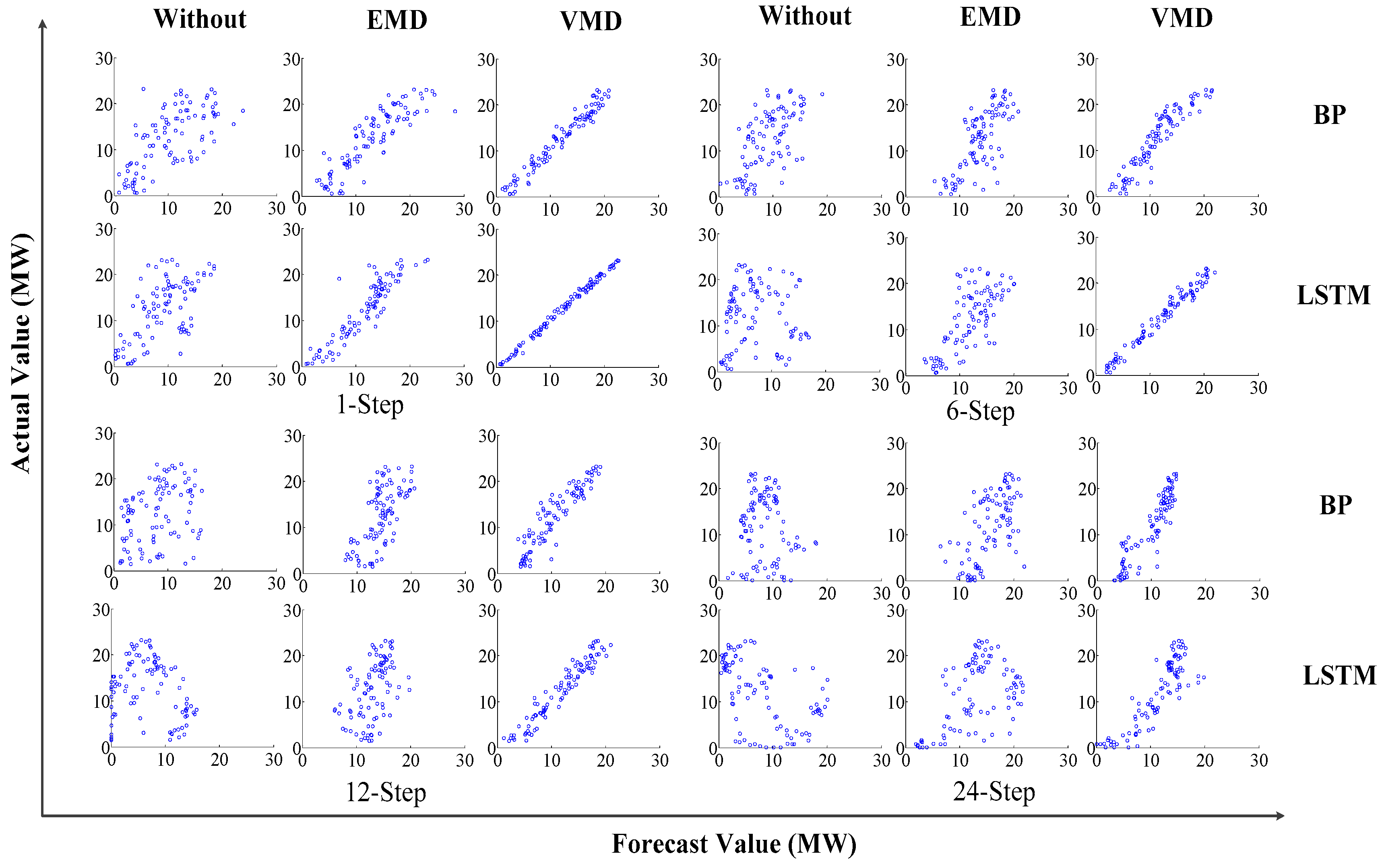
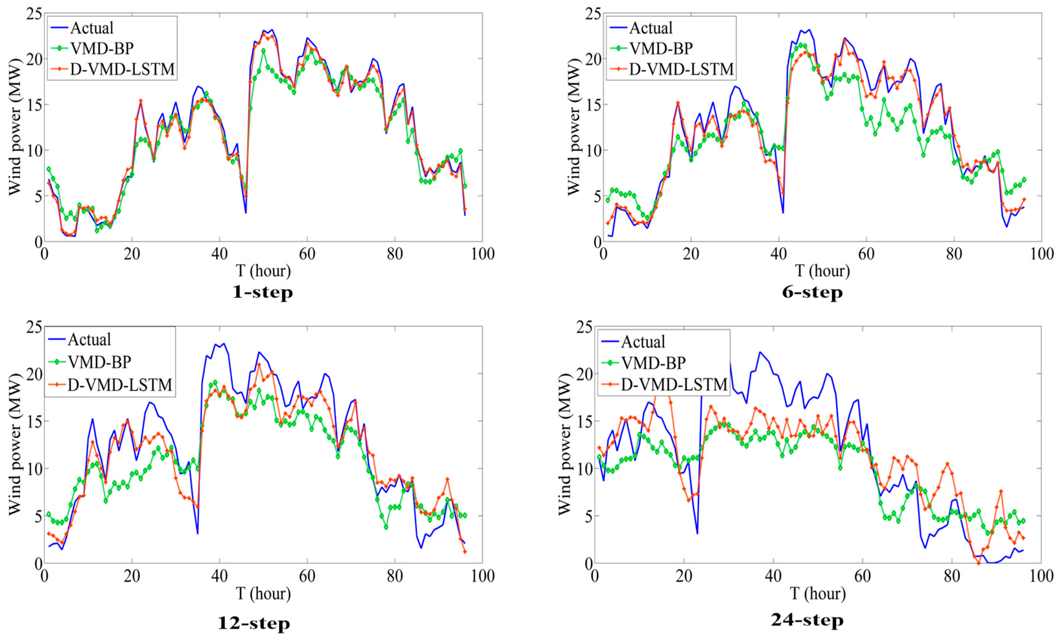
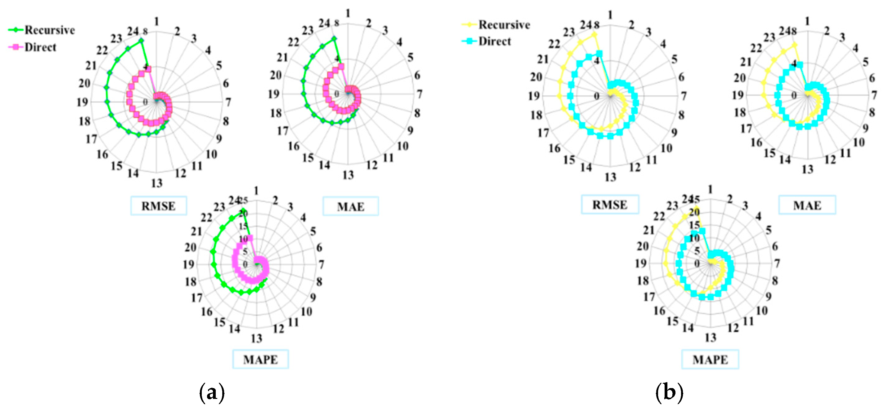
Notably, hourly day-ahead WPF plays a vital role in the wind industry and power markets, because day-ahead forecasting can effectively capture the dynamic behavior of wind power in the future, which is crucial for improving the security and economic benefits of a wind power system. Since multi-step day-ahead forecasting may accumulate forecast errors with the increasing numbers of horizons in real applications, big multi-step forecasting is much more difficult and complicated than the multi-step WPF (below six steps). In order to improve the forecasting accuracy, this paper proposes R (recursive)-VMD-LSTM and D (direct)-VMD-LSTM models on the basis of VMD and LSTM. In contrast to the aforementioned research, this study makes three novel contributions to the field. (1) The combined method proposed pursues the multi-step prediction accuracy of wind power. Specifically, the VMD technique and the combination of several base methods are implemented simultaneously to develop a multi-leveled, combined method. (2) As a well-known deep learning algorithm, the LSTM network is widely used to complete the forecasting for the sub-layers obtained by the VMD, which has satisfactory performance in long-short term dependencies. Owing to the advantages of LSTM, the outputs can directly depend on previous computations as well as calculations of the current time step. (3) To evaluate the hourly day-ahead wind power prediction performance of the combined method, the direct and recursive multi-step prediction mathematical theories are first adopted to establish the R-VMD-LSTM model and D-VMD-LSTM model for comparison. The two LSTM models can learn the correlation relationships through integrating the decomposed modes into the input of one model, which improves the overall forecast accuracy.

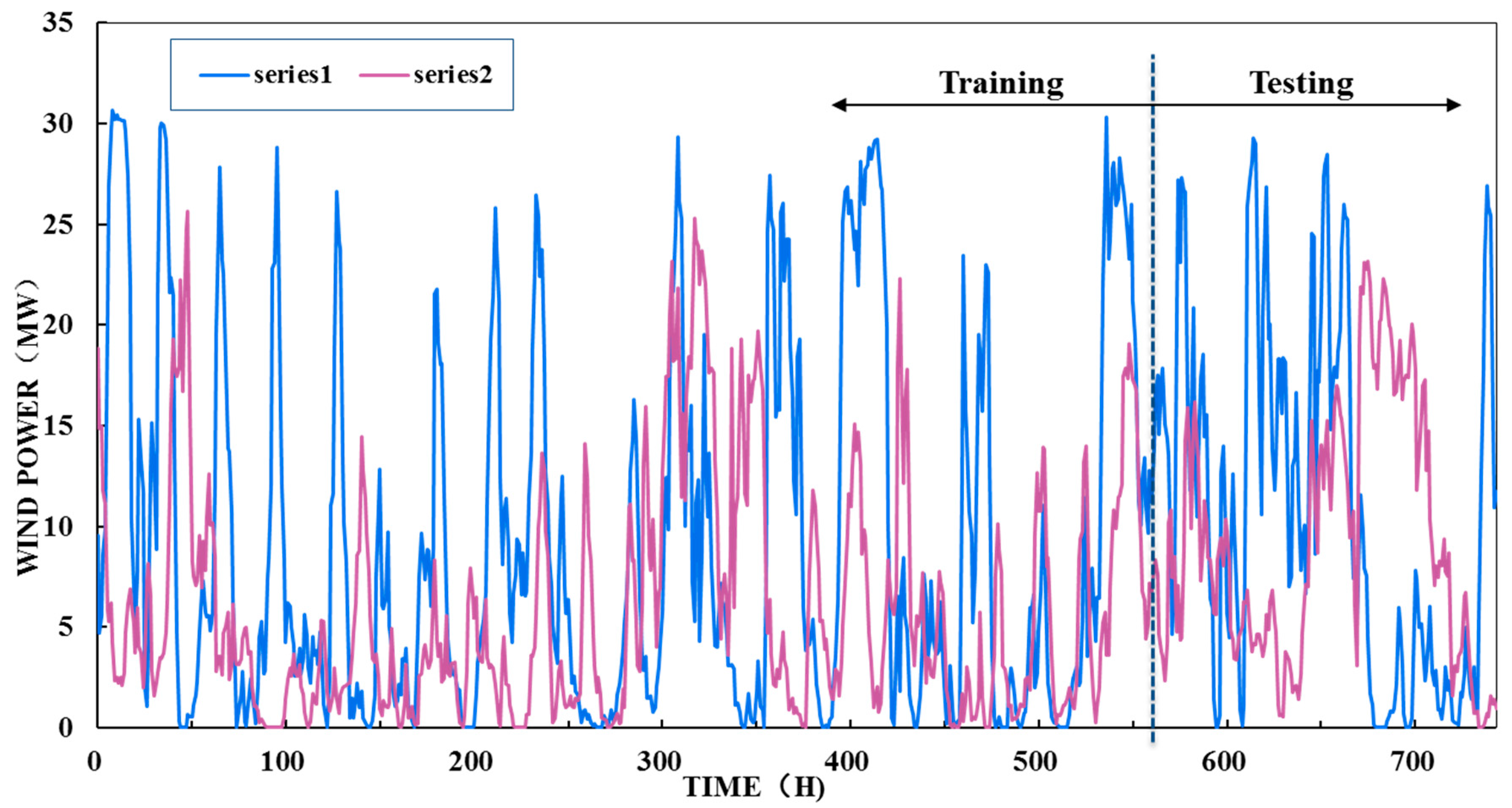
The rest of this paper is organized as follows. Section 2 introduces the procedure of the proposed methods and gives brief descriptions of the required individual algorithms. In Section 3, the R-VMD-LSTM and D-VMD-LSTM models are described. Section 4 provides the experimental results of two series. Finally, Section 5 concludes this paper.

2. Materials and Methods

2.1. The Whole Process of the VMD-LSTM Method

The combined method to forecast wind power is established based on the concept of decomposition and deep learning. On the other hand, the future generated wind power is estimated using previous historical data. The structure of the VMD-LSTM method is depicted in Figure 1, the process of which can be explained as follows [26]:

(1)

The LSTM neural network, with three hidden layers serving as efficient and fast learning machine tools, is adopted to complete the forecasting for each decomposed mode obtained by VMD. LSTM is utilized as the prediction core of the proposed forecasting engine to extract the complicated input–output mapping between historical and forecasting data. Thus, the number of required LSTMs is equal to the number of decomposed modes. The output of each LSTM denotes the forecasted wind power of the same mode order. The LSTM neural network is described in Section 2.2.

(2)

VMD is adopted to decompose the original wind power series into m modes with different frequencies. The analysis of the time series of wind power can be helpful for the precise modeling of its intermittent characteristics. These modes are then used to construct training patterns and forecasted outputs. The details of VMD are presented in Section 2.3.

(3)

The prediction results of the mode values are summed as the ultimate prediction of wind power by the wind farm.

2.2. LSTM Network

Due to the limited computing power and the large amount of data acquisition, deep learning has only been widely concerned and applied in the last two years. LSTM is a type of deep learning algorithm that is an extended version of recurrent neural networks (RNNs). Different from RNN, LSTM has three gates and a memory cell, which are used to control the information in the hidden neuron. The bidirectional RNN (BRNN) is proposed from the directional neural network structure, which can be used for training forward neural networks and backward neural networks. Hence, the output is calculated based on the output state of the hidden layers of forward neural networks and backward neural networks [18]. Figure 2 is a schematic diagram of the structure of the RNN bidirectional cyclic neural network, which is one of the earliest RNN architectures. Figure 3 shows the directional recurrent neural network structures and its structure development diagram. However, the gradient problem in the RNN neural network, which exists widely in forward propagation and backward propagation, may occur when the training gradient cannot be transmitted in the long sequence. Eventually, the neural network will not be able to learn the internal complete information of data acquisition. It is noted that the special structure of LSTM neurons successfully solved the defect gradient uncertainty problem (gradient blasting and gradient disappearance) of the traditional loop neural network during the model training [18]. Figure 4 shows the core difference between RNN and LSTM, and displays the special hidden unit of LSTM.

As shown in Figure 4, the input gate permits inputs to modify the memory cell state, the output gate allows or obstructs the memory cell state from influencing other neurons, and the memory cell can impede outside interference, which further allows the LSTM model to learn time series with long spans. The i, f, and o represent the input, forget, and output gates, respectively. The c and $\overline{c}$ represent the memory cell state and the new memory cell gate, respectively. The mathematical representation of LSTM can be obtained as [27]:

Input gate (i_t, which decides the information to be added to the cell):

$$i_t=\sigma ({\omega }_i\ast x_t+U_i\ast s_{t-1}+V_i^o{c}_{t-1}+b_i)$$

(1)

Forget gate (f_t, which decides the information to be deleted from the cell):

$$f_t={\sigma }_g({\omega }_f\ast x_t+U_f\ast s_{t-1}+V_f^o{c}_{t-1}+b_f)$$

(2)

Output gate (o_t, which decides the information to be exported from the cell):

$$o_t={\sigma }_g({\omega }_o\ast x_t+U_o\ast s_{t-1}+V_o^o{c}_{t-1}+b_o)$$

(3)

Cell:

$$c_t=f_t^o{c}_{t-1}+i_t^o{\overline{c}}_t$$

(4)

$${\overline{c}}_t={\sigma }_c(W_c\ast x_t+U_c\ast s_{t-1}+b_c)$$

(5)

Output vector:

$$s_t=o_t^o{\sigma }_h(c_t)$$

(6)

where x_t is the input vector. W, U, V, and b are parameters for weights and biases. ° denotes the scalar product of two vectors; ${\sigma }_g$ is the sigmoid function; and ${\sigma }_h$ and ${\sigma }_c$ are the hyperbolic tangent functions. For a given input z, the output of the hyperbolic tangent function is:

$$f(z)=\frac{e^z-e^{-z}}{e^z+e^{-z}}$$

(7)

LSTM is implemented using Keras and Tensorflow. Keras is a Python-based high-level deep learning library. It runs on top of TensorFlow or Theano. TensorFlow is an open-source deep learning software released by Google in 2016. Under the Apache 2.0 and open-source code specifications, all developers can use it [28].

2.3. VMD

VMD is a newly developed multi-resolution technique for adaptive and non-recursive signal decomposition. Its overall solution process is the construction and solution of the variational problem. Each mode can be compacted around a center pulsation that is determined during the decomposition process. This involves decomposing a real valued signal into different modes called u_k, which have specific sparsity properties, while reproducing the main signal. Each mode compacts with a central frequency of ω_k and has limited bandwidth [28,29,30,31]. The solution of the sub-signal u_k(t) is as follows:

(1)

According to the Hilbert transform, the corresponding analytic signal of each sub-modal u_k(t) is calculated, so that the single-side spectrum can be obtained.

(2)

By mixing the index $e^{-j{\omega }_{k}t}$ of each modal analytical signal corresponding center frequency ω_k, the sub-modal signal u_k(t) spectrum is changed to the base frequency band.

(3)

The norm of the square of the demodulation signal gradient L² is calculated to estimate the width of the sub-modal signal u_k(t). The variational problem with constraint is:

$$\{\begin{array}{l}\underset{\left\{u_k\right\},\left\{{\omega }_k\right\}}{Min}\{{\displaystyle \sum _{k=1}^K{\Vert {\partial }_t[(\delta (t)+\frac{j}{\pi t})\otimes u_k(t)]e^{-j{\omega }_{k}t}\Vert }_2^2}\\ s.t.{\displaystyle \sum _{k=1}^K{u}_k=f}\end{array}$$

(8)

where {u_k} and {ω_k} represent the set of sub-signals and its corresponding central frequency, k is the total number of sub-signals, δ(t) is the Dirac distribution, and $\otimes$ represents the convolution operation.

Here, the quadratic penalty factor and Lagrange multiplier α are used to transform Equation (8) to an unconstrained optimization problem. The formula is as follows:

$$L\left(\left\{u_k\right\},\left\{{\omega }_k\right\},\lambda \right)=\alpha {{\displaystyle \sum _{k=1}^K\Vert {\partial }_t[(\delta (t)+\frac{j}{\pi t})\times u_k(t)]e^{-j{\omega }_{k}t}\Vert }}_2^2+\langle \lambda (t),f(t)-{\displaystyle \sum _{k=1}^K{u}_k(t)\rangle }$$

(9)

where α is the balance parameter, which is used to guarantee the reconstruction accuracy of the signal in the presence of Gaussian noise, and λ is the Lagrange multiplier, which is used to maintain the rigor of the constraint conditions.

The minimization problem of Equation (8) is transformed into a series of sub-optimization problems, which are expressed by Equation (9). The multiplier alternating direction method is used to solve the problem, and the solution is as follows:

$${\widehat{u}}_k^{n+1}(\omega )=\frac{f(\omega )-{\displaystyle {\sum }_{i\ne k}{\widehat{u}}_i^n(\omega )+\frac{\widehat{\lambda }(\omega )}{2}}}{1+2\alpha {(\omega -{\omega }_k^n)}^2}$$

(10)

$${\omega }_k^{n+1}=\frac{{\displaystyle {\int }_0^{\infty }\omega {\left|{\widehat{u}}_k^n(\omega )\right|}^{2}d\omega }}{{\displaystyle {\int }_0^{\infty }{\left|{\widehat{u}}_k^n(\omega )\right|}^{2}d\omega }}$$

(11)

where $\widehat{f}(\omega )$, ${\widehat{u}}_i^n(\omega )$, $\widehat{\lambda }(\omega )$, and ${\widehat{u}}_k^{n+1}(\omega )$ respectively represent the Fourier transform of f(t), $u_i^n(\omega )$, $\lambda (t)$, $u_k^{n+1}(t)$, and $u_k^{n+1}(t)$. ${\widehat{u}}_k^{n+1}(\omega )$ is equivalent to the Wiener filter of the current remaining component $f(\omega )-{\displaystyle {\sum }_{i\ne k}{\widehat{u}}_i^n(\omega )+\frac{\widehat{\lambda }(\omega )}{2}}$. $u_k^{n+1}(\omega )$ represents the focus center of the current modal function. n is the number of iterations. The steps of variational modal decomposition are as follows:

(1)

Initialize $\left\{{\omega }_k^1\right\}$, $\left\{{\widehat{u}}_i^n\right\}$, and $\left\{{\widehat{\lambda }}_k^1\right\}$, set the number of iterations to 1.

(2)

For each sub-signal, according to Equations (10) and (11), update operations to obtain ${\widehat{u}}_k^{n+1}(\omega )$ and ${\omega }_k^{n+1}$.

(3)

Update the Lagrange multiplier according to Equation (12):

$${\widehat{\lambda }}^{n+1}(\omega )={\widehat{\lambda }}^n(\omega )+\tau \left(\widehat{u}(\omega )-{\displaystyle \sum _{k=1}^K{\widehat{u}}_k^{n+1}(\omega )}\right)$$

(12)

where τ is the update parameter.

(4)

The decomposition process ends when the convergence condition is satisfied; otherwise, the iteration number is updated, and the process returns to Step 2.

$${\displaystyle \sum _{k=1}^K\frac{{\Vert {\widehat{u}}_k^{n+1}-{\widehat{u}}_k^n\Vert }_2^2}{{\Vert {\widehat{u}}_k^n\Vert }_2^2}}<\epsilon$$

(13)

2.4. Performance Evaluation Index

Three evaluation indexes were chosen to evaluate the prediction performance of the proposed model [5].

The mean absolute error (MAE) can be defined as:

$$MAE=\frac{1}{N}{\displaystyle \sum _{t=1}^N\left|e_{t+k/t}\right|}$$

(14)

where e_t+k/t denotes the prediction errors and can be defined as:

$$e_{t+k/t}=V_{t+k}-{\widehat{V}}_{t+k/t}$$

(15)

where V_t+k and ${\widehat{V}}_{t+k/t}$ are the actual and predicted wind power, MW.

The mean absolute percentage error (MAPE) can be defined as:

$$MAPE=\frac{1}{N}{\displaystyle \sum _{t=1}^N\left|\frac{e_{t+k/t}}{P_{cap}}\right|}$$

(16)

where P_cap denotes the installed capacity of the wind farm.

The RMSE can be defined as:

$$RMSE=\sqrt{\frac{1}{N}{\displaystyle \sum _{t=1}^N{(e_{t+k/t})}^2}}$$

(17)

3. R-VMD-LSTM and D-VMD-LSTM Models

A neural network model for small multi-step wind power prediction is extensive, but big multi-step methods are relatively few, mainly due to the limitations of traditional neural network internal structures and computer operating performance. With the rapid development of computer parallel computing technology and the widespread use of deep learning, the LSTM neural network was introduced for big multiple steps prediction due to its special network structure, as described in detail in Section 2.3. Therefore, on the basis of the combined method, in this study, R-VMD-LSTM and D-VMD-LSTM are proposed for hourly day-ahead WPFs. The model architectures are demonstrated in Figure 5.

3.1. R-VMD-LSTM

Wind power hourly data formally lined up as a time series in hours. This time series $[P_1,P_2,\dots ,P_N]$, which is composed of N observations, is used for forecasting wind power for s steps (hours) ahead, given as $[P_{N+1},P_{N+2},\dots ,P_{N+S}]$, where s denotes the absolute forecasting horizon. The basis of any forecasting strategy is that the predicted power ($P^{\prime }$) can be shown as a function of past values (P).

In the R-VMD-LSTM model, first, a single model $f_r(·)$ is trained to perform a one-step ahead forecast, i.e.,

$$P_{t+1}^{\prime }=f_r(P_t,P_{t-1},\dots ,P_{t-d+2},P_{t-d+1})+\omega$$

(18)

where $f_r(·)$ represents the recursive relationship between $P_{t+1}^{\prime }$ and $P_t,P_{t-1},\dots ,P_{t-d+2},P_{t-d+1}$; $P_{t+1}^{\prime }$ denotes the first-step forecasted wind power; $P_t,P_{t-1},\dots ,P_{t-d+2},P_{t-d+1}$ denotes the historical wind power; d denotes the number of previous inputs of the series; and ω denotes the bias.

For t steps, step one is predicted by using the model in Equation (18). Afterwards, the forecasted value is included as the latest entry of the input data to predict the next step using the same trained model. This procedure is repeated for the horizon s and input length d. The established recursive forecasting models are described as:

$$\{\begin{array}{c}{P}_{t+1}^{\prime } =f_r(P_t,P_{t-1},\dots ,P_{t-d+2},P_{t-d+1})\hfill \\ P_{t+2}^{\prime }=f_r(P_{t+1}^{\prime },P_t,\dots ,P_{t-d+1},P_{t-d})\hfill \\ \hfill ⋮\hfill \\ P_{t+s}^{\prime }=f_r(P_{t+s-1}^{\prime },P_{t+s-2}^{\prime },\dots ,P_{t+1}^{\prime },P_t)\hfill \end{array}$$

(19)

where $P_{t+1}^{\prime },P_{t+2}^{\prime },\dots ,P_{t+s}^{\prime }$ denote the one-step ahead, two-steps ahead and s-steps ahead forecasted wind power, respectively; and 24 was selected for s in the recursive day-ahead forecasting model.

3.2. D-VMD-LSTM

The D-VMD-LSTM model is based on the principle that each step is independent from the others. Hence, a separate function model is trained for each forecasting horizon, with a total number of models for the entire forecasting horizon. For big multi-step forecasts, a recursive model may be potentially inaccurate because of the accumulation of forecast error with each forecasted value.

The D-VMD-LSTM model is described as:

$$(P^{t+1},P^{t+2},\dots ,P^{t+\mathrm{s}})= f_d(P^t,P^{t-1},\dots ,P^{t-d+1})+\omega$$

(20)

where $f_d(·)$ represents the direct relationship between $P^{t+1},P^{t+2},\dots ,P^{t+\mathrm{s}}$ and $P^t,P^{t-1},\dots ,P^{t-d+1}$; $P^{t+1},P^{t+2},\dots ,P^{t+\mathrm{s}}$ are the forecasted data; $P^t,P^{t-1},\dots ,P^{t-d+1}$ are the historical data; d denotes the number of previous inputs of the series; s represents the horizon during forecasting (24 was selected for s in the direct day-ahead forecasting model), and ω denotes the bias.

4. Results

4.1. Experimental Date Description

This paper adopts two series of hourly wind power collected respectively in summer (1–31 August 2017) and spring (1–31 March 2017) from a wind farm located in Henan, China to evaluate the effectiveness of the proposed models (Figure 6). Due to the different climatic features in summer and spring, these series have obviously different characteristics. Hence, the sets adopted in this paper can comprehensively and systematically evaluate the effectiveness and practicability of the proposed models. In addition, in each dataset, the observation numbers 1–576 (24 days) and 577–744 (7 days) are respectively adopted as the training and testing sets. It should be noted that all of the prediction simulations are implemented in Python 3.x.

4.2. Parameter Selection

In this study, BP, ELM, and SVM are utilized to evaluate the performance of the proposed models.

Table 1. The initial parameters of back propagation (BP), extreme learning machine (ELM), support vector machine (SVM), and LSTM.

Algorithm	Parameters	Value
BP/ELM	Maximum iterations	200
	Learning rate	0.1
	Momentum operator	0.9
	Hidden layer neurons	30
SVM	Penalty factor	48.8
	Gamma	0.06
	Loss function	0.01
LSTM	Batch size	10
	Maximum iterations	200
	LSTM layer neurons	48
	Dropout layer neurons	48
	Hidden layer neurons	60

represents the main parameters of BP, ELM, SVM, and LSTM. To demonstrate the superiority of the R-VMD-LSTM and D-VMD-LSTM models over the benchmarked models, comparisons between the proposed models and EMD-BP, EMD-ELM, EMD-SVM, EMD-LSTM, VMD-BP, VMD-ELM, and VMD-SVM are made.

In addition to the parameters of the above-mentioned models, the selection of candidate input also has a crucial impact on the prediction accuracy of a given model. In the proposed models, the forecast interval is 1 h, and forecast horizons are 24 h. Thus, the time interval between two original series of wind power is 1 h, and the forecast engine predicts the next 24 h of wind farm-produced power. The hourly lagged values of wind farm-produced power in the past 24 h (one day), 48 h (two days) and 72 h (three days) are considered as candidate input. Each candidate vector of input length has 24 points, 48 points (24 × 2), and 72 points (24 × 3), respectively. The comparison and evaluation of three candidate input lengths based on the LSTM model are shown in

Table 2. Comparison and evaluation of different input lengths in the LSTM model. MAPE: mean absolute percentage error.

Input Lengths	24 Points (One-Day Ahead)	48 Points (Two-Days Ahead)	72 Points (Three-Days Ahead)
RMSE (MW)	8.8	7.6	8.2
MAE (MW)	7.0	6.4	6.9
MAPE (%)	23	21	23

. The RMSE, MAE, and MAPE of 48 points are 7.6 MW, 6.4 MW, and 21%, showing that 48 points provided the best performance of the three candidate input lengths.

4.3. Analysis of Proposed Models

4.3.1. Decomposed Results by VMD

In order to improve the overall predicting performance, this paper adopts the VMD technique to decompose the original series into a number of components. The data decomposition results are listed in Figure 7 and Figure 8. Specifically, the first 576 data observations of each mode are used as the training sets for the forecast model.

VMD is a completely non-recursive decomposition model, in which all of the modes are extracted concurrently. However, the model requires a preset mode number k, which limits the adaptability of the method, since a large deviation in the number of modes will cause some modes to be discarded or cause the mixing of modes. Hence, the ratio of residual energy to the original signal energy was introduced as an optimization index in the VMD technique, which is the residual error after the decomposition of the original signal [31]. The final mode number was determined when the ratio was less than 1%. The ratio of residual energy under a different mode number by VMD is presented in

Table 3. The ratio of residual energy with different mode numbers by VMD.

Mode Number	3	5	7	9	11	15	20	25	30	40
Series 1 (MAPE, %)	4.5	3.7	2.6	2.2	1.62	1	0.7	0.6	0.6	0.5
Series 2 (MAPE, %)	6.4	4.9	4.1	2.7	2.3	2.1	1.2	1	0.9	0.6

. The formula is as follows:

$$MAPE=\frac{1}{N}{\displaystyle \sum _{t=1}^N\left|\frac{f-{\displaystyle \sum _K{u}_k(t)}}{f}\right|}$$

(21)

where f and u_k(t) denote the original wind power series and the mode, respectively.

4.3.2. Recursive Hourly Day-Ahead Forecasting

To validate the prediction performance of the R-VMD-LSTM model, eight models are employed for comparison: the LSTM model, the ELM model, the SVM model, the EMD-ELM model, the EMD-SVM model, the EMD-LSTM, the VMD-SVM model, and the VMD-ELM model. The evaluation indexes of the proposed and comparison models are presented in

Table 4. Performance evaluations of recursive hourly day-ahead forecasting models for series 1. EMD: empirical mode decomposition.

Models	Indexed	1-Step	6-Step	12-Step	24-Step
ELM	RMSE (MW)	3.39	8.61	9.46	9.01
	MAE (MW)	2.48	6.92	8.19	7.94
	MAPE (%)	8	23	27	26
SVM	RMSE (MW)	4.98	9.11	9.96	9.64
	MAE (MW)	3.87	7.71	8.94	8.18
	MAPE (%)	13	26	30	27
LSTM	RMSE (MW)	3.67	7.24	7.27	8.39
	MAE (MW)	2.81	6.02	5.88	6.72
	MAPE (%)	9	20	20	22
EMD-ELM	RMSE (MW)	1.74	4.14	6.41	5.87
	MAE (MW)	1.26	3.48	5.12	4.44
	MAPE (%)	4	12	17	15
EMD-SVM	RMSE (MW)	1.89	4.83	7.07	5.37
	MAE (MW)	1.38	3.74	5.8	4.34
	MAPE (%)	5	12	19	14
EMD-LSTM	RMSE (MW)	1.54	2.9	4.08	11.92
	MAE (MW)	1.19	2.27	3.37	10.33
	MAPE (%)	4	8	11	34
VMD-ELM	RMSE (MW)	0.85	1.56	2.09	5.77
	MAE (MW)	0.66	1.3	1.65	4.6
	MAPE (%)	2	4	5.5	15.2
VMD-SVM	RMSE (MW)	0.79	1.75	2.72	3.61
	MAE (MW)	0.65	1.41	2.29	3.19
	MAPE (%)	2.2	4.7	7.6	10.6
R-VMD-LSTM	RMSE (MW)	0.35	0.92	2.97	7.16
	MAE (MW)	0.28	0.72	2.51	6.44
	MAPE (%)	1	2	8	22

. Figure 9 shows the scatter plot of the observed values and forecasting values for different recursive models. Also, the forecasting results based on the R-VMD-LSTM, VMD-ELM, and VMD-SVM models are shown in Figure 10.

Based on the forecasting error results shown in Table 4, the following can be observed. (a) The comparison between without (without decomposition), EMD, and VMD prediction models show that the models combined with VMD are effective in boosting the forecasting accuracy. This is because the VMD model is helpful in modeling the data stochastic volatility. (b) A comparison is conducted among LSTM, ELM, and SVM. The results indicate that the deep learning approaches are more effective than the conventional machine learning method in enhancing the forecasting accuracy due to the directional loop neural network structure and special hidden unit. (c) The R-VMD-LSTM model performs better than the VMD-ELM and VMD-SVM models in the recursive forecasting. However, as the step increases, the accuracy of the R-VMD-LSTM model is decreasing, and its RMSE, MAE, and MAPE range from 0.35 MW, 0.28 MW, and 1% to 7.16 MW, 6.44 MW, and 22% from Step 1 to Step 24, respectively.

4.3.3. Direct Hourly Day-Ahead Forecasting

In the direct forecasting model, BP and LSTM are used to establish the hybrid methods (EMD-BP, VMD-BP, EMD-LSTM, and D-VMD-LSTM) for comparison. The evaluations are summarized in

Table 5. Performance evaluations of direct hourly day-ahead forecasting models for Series 1.

Models	Indexed	1-Step	6-Step	12-Step	24-Step
BP	RMSE (MW)	5.32	6.01	7.76	8.75
	MAE (MW)	4.35	5.00	6.57	7.93
	MAPE (%)	15	17	22	26
LSTM	RMSE (MW)	6.06	9.51	10.34	12.08
	MAE (MW)	5.04	8.19	9.32	10.83
	MAPE (%)	17	27	31	36
EMD-BP	RMSE (MW)	3.16	4.78	5.29	6.9
	MAE (MW)	2.54	3.9	4.4	5.61
	MAPE (%)	8	13	15	19
EMD-LSTM	RMSE (MW)	2.91	4.55	5.61	6.57
	MAE (MW)	2.1	3.49	4.71	5.78
	MAPE (%)	7	12	16	19
VMD-BP	RMSE (MW)	1.69	2.98	3.36	4.46
	MAE (MW)	2.1	3.49	4.71	5.78
	MAPE (%)	4	8	9	12
D-VMD-LSTM	RMSE (MW)	0.67	1.30	2.17	3.86
	MAE (MW)	0.54	1.00	1.70	3.21
	MAPE (%)	2	3	6	10

, and the forecasting results are shown in Figure 11 and Figure 12. From Table 5, the following can be observed. (a) Similar to the use in the recursive hourly day-ahead prediction study, VMD and LSTM are effective in direct forecasting. (b) The D-VMD-LSTM model performs better than the VMD-BP model, which provides the forecasting performances of the proposed and other comparison models over horizons. Specifically, the RMSE, MAE, and MAPE range from 1.56 MW, 1.26 MW, and 4% to 5.91 MW, 4.66 MW, and 16% between Step 1 and Step 24, respectively. The results indicate that the D-VMD-LSTM model can improve the accuracy of hourly day-ahead predictions to a great extent.

4.4. Contrast Analysis between R-VMD-LSTM and D-VMD-LSTM Models

As a further investigation, in this section, wind power Series 1 and 2 are adopted to make direct and recursive hourly day-ahead predictions using R-VMD-LSTM and D-VMD-LSTM model comparisons and analyses.

Table 6. The hourly day-ahead forecasting results of the D-VMD-LSTM model of Series 1 and 2. MAE: mean absolute error; and RMSE: root mean square error.

Step Number	Series 1			Series 2
	RMSE (MW)	MAE (MW)	MAPE (%)	RMSE (MW)	MAE (MW)	MAPE (%)
1-step	0.67	0.54	1.80	1.15	0.92	3.10
2-step	0.75	0.61	2.00	1.4	1.12	3.70
3-step	0.91	0.72	2.40	1.73	1.45	4.80
4-step	1.04	0.82	2.70	2.04	1.71	5.70
5-step	1.16	0.9	3.00	2.31	1.96	6.50
6-step	1.3	1	3.30	2.56	2.16	7.20
7-step	1.42	1.12	3.70	2.86	2.42	8.10
8-step	1.55	1.24	4.10	3.14	2.61	8.70
9-step	1.77	1.42	4.70	3.31	2.78	9.30
10-step	1.92	1.5	5.00	3.57	3.04	10.10
11-step	2.03	1.59	5.30	3.86	3.29	11.00
12-step	2.17	1.7	5.70	4.26	3.65	12.20
13-step	2.34	1.85	6.20	4.55	3.95	13.20
14-step	2.52	2.02	6.70	4.66	4.09	13.60
15-step	2.63	2.13	7.10	4.68	4.09	13.60
16-step	2.69	2.18	7.30	4.69	3.98	13.30
17-step	2.83	2.28	7.60	4.63	3.86	12.90
18-step	3.05	2.47	8.20	4.71	3.91	13.00
19-step	3.27	2.69	9.00	4.74	3.9	13.00
20-step	3.4	2.82	9.40	4.75	3.82	12.70
21-step	3.52	2.95	9.80	4.87	3.85	12.80
22-step	3.63	3.03	10.10	5.12	4	13.30
23-step	3.69	3.08	10.30	5.07	3.99	13.30
24-step	3.86	3.21	10.70	4.94	3.89	13.00

and Figure 13 show that the errors of R-VMD-LSTM and D-VMD-LSTM range from step one to Step 24 of Series 1 and 2, respectively. In order to more clearly analyze the results of the D-VMD-LSTM model, the multi-step histogram of the forecasting error of Series 1 and 2 by the proposed model is described in Figure 14 and Figure 15.

From Table 6 and Figure 13 and Figure 14, the following can be concluded. (a) The R-VMD-LSTM model gives a more accurate prediction at the beginning of a day, while the D-VMD-LSTM model gives a more accurate prediction at the end of a day. For instance, the MAPE of the D-VMD-LSTM model is below 20% from step one to Step 24 for both Series 1 and 2. Therefore, the D-VMD-LSTM model can satisfy the bidding price requirements in a liberalized power market, as proposed by the NEB in 2011. (b) The prediction error of the D-VMD-LSTM model shows a single peak distribution of “high in the middle and low on both sides”, and the peak at the error zero point of the distribution is concentrated. With the extension of the prediction horizon, the single peak value tends to be low and dwarfing, and the error tends to expand.

5. Discussion and Conclusions

With the large-scale popularization of wind energy, the liberalized power market is undergoing fierce competition. Accurate WPF plays a vital role in energy auction markets and efficient resource planning. Efficient day-ahead forecasting models have to be applied to mitigate the uncertainty of wind energy access to the grid. For existing power systems, although various forecasting models could supply a straightforward solution, their refined planning and the operation of smart grids represent significant constraints.

This paper mainly proposed R-VMD-LSTM and D-VMD-LSTM models for hourly predictions of day-ahead wind power. Compared with the other works, this work focuses more on the characteristics of direct and recursive forecasting, and expands the research to hourly day-ahead forecasts. Based on a novel combined technique, this method shows that the VMD algorithm has an integrating performance as well as good self-adaptive ability to remove the stochastic volatility.

This study also demonstrated that LSTM is able to provide precise time-series predictions for wind power plants. LSTM can be a powerful tool for managers or engineers of electric power systems, who can take advantage of accurate predictions to improve their decision-making. Intelligent wind farms will become the backbone of smart grids. In recent years, deep learning methods have gained more and more success in many fields. In the literature [31], the authors presented a wind speed prediction model based on VMD and the CNN (Convolutional Neural Network), in which the CNN was employed as the predictor. The obtained results show that VMD-CNN achieved significant results, while the SVR-based and ELM-based methods performed poorly. The findings mentioned above are consistent with those in the present study. However, the large amounts of field training data and programming skill behind deep learning limit its application in wind forecasting. The potential power of deep learning is still fascinating, and more studies about absorbing deep learning into the wind energy field are necessary.

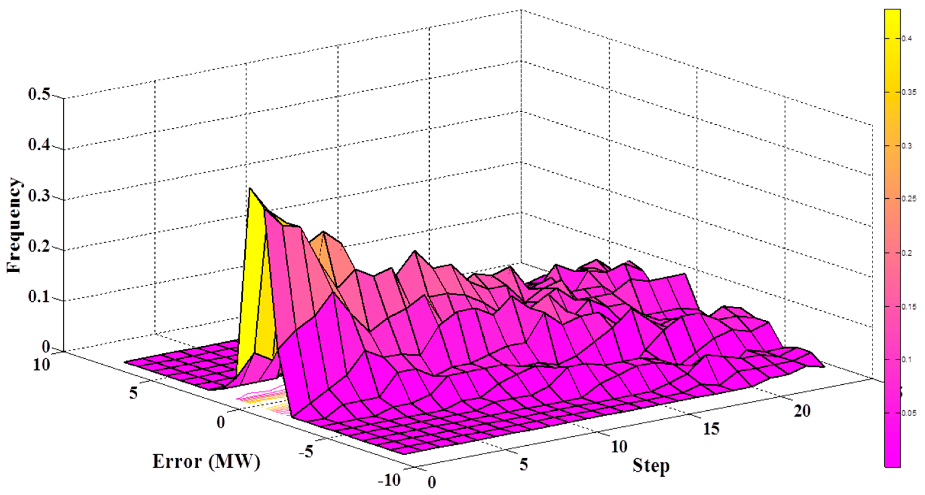
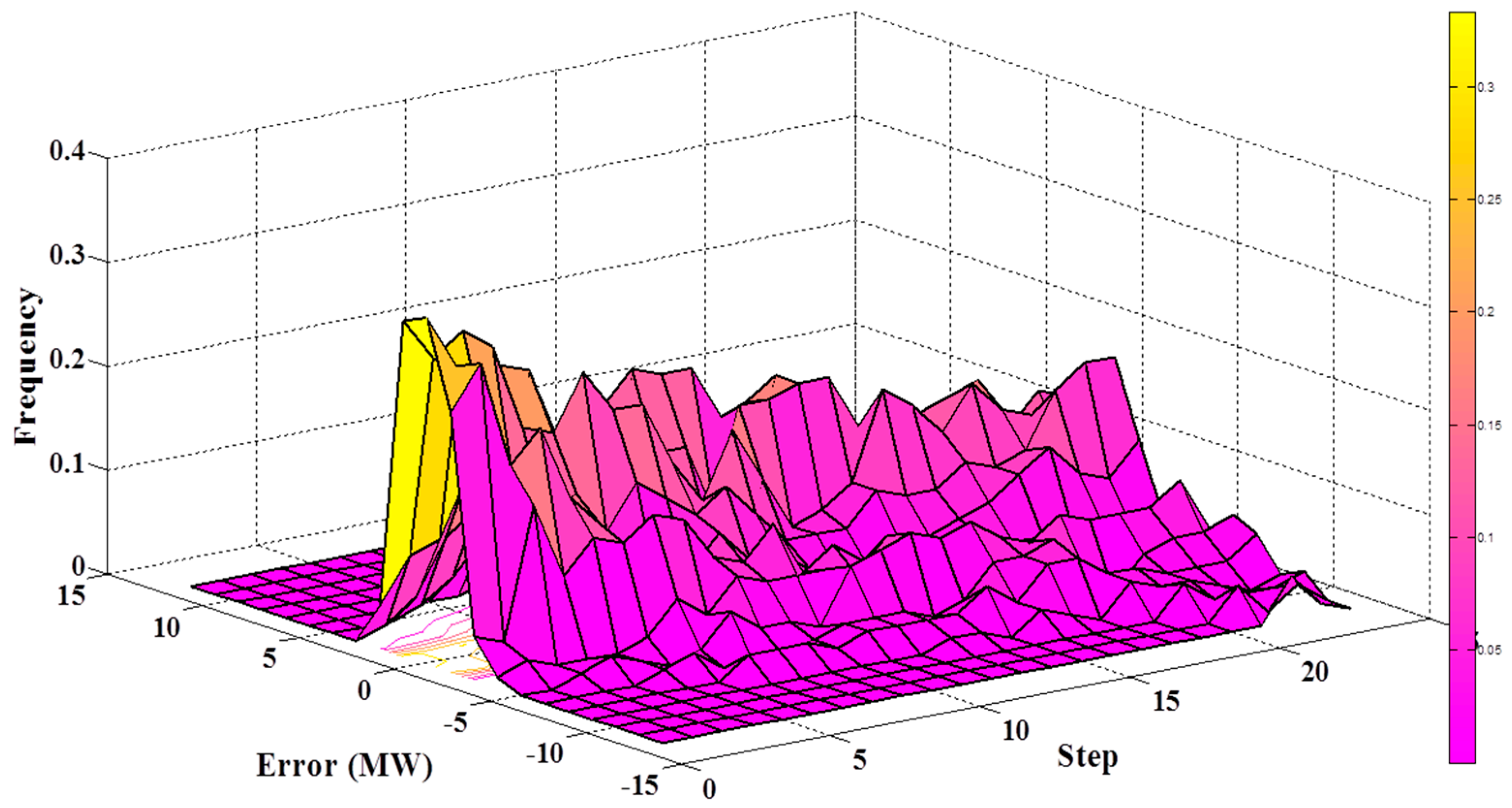
In future research, we will focus more on realizing WPF at different step errors and with a changing numbers of steps using R-VMD-LSTM and D-VMD-LSTM.

References

1. Gallego-Castillo, C.; Cuerva-Tejero, A.; Lopez-Garcia, O. A review on the recent history of wind power ramp forecasting. Renew. Sustain. Energy Rev. 2015, 52, 1148–1157. [Google Scholar] [CrossRef] [Green Version]
2. Fang, W.; Huang, S.Z.; Huang, G.H.; Huang, Q.; Wang, H.; Wang, L.; Zhang, Y.; Li, P.; Man, L. Copulas-based risk analysis for inter-seasonal combinations of wet and dry conditions under a changing climate. Int. J. Clim. 2018. [Google Scholar] [CrossRef]
3. Liu, S.Y.; Huang, S.Z.; Xie, Y.Y.; Wang, H.; Leng, G.Y.; Huang, Q.; Wei, X.T.; Wang, L. Identification of the non-stationary of floods: Changing patterns, causes, and implications. Water Res. Manag. 2018. [Google Scholar] [CrossRef]
4. Sarshar, J.; Moosapour, S.S.; Joorabian, M. Multi-objective energy management of a micro-grid considering uncertainty in wind power forecasting. Energy 2017, 139, 680–693. [Google Scholar] [CrossRef]
5. De Queiroz, A.R. Stochastic hydro-thermal scheduling optimization: An overview. Renew. Sustain. Energy Rev. 2016, 62, 382–395. [Google Scholar] [CrossRef]
6. China Energy Storage Network News Center. Available online: www.escn.com.cn (accessed on 9 October 2018). (In Chinese).
7. Wang, C.; Li, X.; Wang, Z.; Dong, X.; Liang, Z.; Liu, X.; Liang, J.; Han, X. Day-ahead unit commitment method considering time sequence feature of wind power forecast error. Int. J. Electr. Power Energy Syst. 2018, 98, 156–166. [Google Scholar] [CrossRef]
8. Zhao, X.; Liu, J.; Yu, D.; Chang, J. One-day-ahead probabilistic wind speed forecast based on optimized numerical weather prediction data. Energy Convers. Manag. 2018, 164, 560–569. [Google Scholar] [CrossRef]
9. Wang, J.; Song, Y.; Liu, F.; Hou, R. Analysis and application of forecasting models in wind power integration: A review of multi-step-ahead wind speed forecasting models. Renew. Sustain. Energy Rev. 2016, 60, 960–981. [Google Scholar] [CrossRef]
10. Zhao, J.; Guo, Z.; Su, Z.; Zhao, Z.; Xiao, X.; Liu, F. An improved multi-step forecasting model based on WRF ensembles and creative fuzzy systems for wind speed. Appl. Energy 2016, 162, 808–826. [Google Scholar] [CrossRef]
11. Tascikaraoglu, A.; Uzunoglu, M. A review of combined approaches for prediction of short-term wind speed and power. Renew. Sustain. Energy Rev. 2014, 34, 243–254. [Google Scholar] [CrossRef]
12. Ahmed, A.; Khalid, M. Multi-step Ahead Wind Forecasting Using Nonlinear Autoregressive Neural Networks. Energy Procedia 2017, 134, 192–204. [Google Scholar] [CrossRef]
13. Niu, T.; Wang, J.; Zhang, K.; Du, P. Multi-step-ahead wind speed forecasting based on optimal feature selection and a modified bat algorithm with the cognition strategy. Renew. Energy 2018, 118, 213–229. [Google Scholar] [CrossRef]
14. Yuan, X.; Tan, Q.; Lei, X.; Yuan, Y.; Wu, X. Wind power prediction using hybrid autoregressive fractionally integrated moving average and least square support vector machine. Energy 2017, 129, 122–137. [Google Scholar] [CrossRef]
15. Aydin, O.; Guldamlasioglu, S. Using LSTM networks to predict engine condition on large scale data processing framework. In Proceedings of the 2017 4th International Conference on Electrical and Electronic Engineering (ICEEE), Ankara, Turkey, 8–10 April 2017; pp. 281–285. [Google Scholar]
16. Srivastava, S.; Lessmann, S. A comparative study of LSTM neural networks in forecasting day-ahead global horizontal irradiance with satellite data. Sol. Energy 2018, 162, 232–247. [Google Scholar] [CrossRef]
17. Liu, H.; Mi, X.; Li, Y. Wind speed forecasting method based on deep learning strategy using empirical wavelet transform, long short term memory neural network and Elman neural network. Energy Convers. Manag. 2018, 156, 498–514. [Google Scholar] [CrossRef]
18. Qu, X.; Kang, X.; Zhang, C.; Jiang, S.; Ma, X. Short-Term Prediction of Wind Power Based on Deep Long Short-Term Memory. In Proceedings of the 2016 IEEE PES Asia-Pacific Power and Energy Engineering Conference (APPEEC), Xi’an, China, 25–28 October 2016. [Google Scholar]
19. Liu, H.; Mi, X.; Li, Y. Smart multi-step deep learning model for wind speed forecasting based on variational mode decomposition, singular spectrum analysis, LSTM network and ELM. Energy Convers. Manag. 2018, 159, 54–64. [Google Scholar] [CrossRef]
20. Li, H.; Wang, J.; Lu, H.; Guo, Z. Research and application of a combined model based on variable weight for short term wind speed forecasting. Renew. Energy 2018, 116, 669–684. [Google Scholar] [CrossRef]
21. Zhao, J.; Guo, Y.; Xiao, X.; Wang, J.; Chi, D.; Guo, Z. Multi-step wind speed and power forecasts based on a WRF simulation and an optimized association method. Appl. Energy 2017, 197, 183–202. [Google Scholar] [CrossRef]
22. Guo, Z.; Zhao, W.; Lu, H.; Wang, J. Multi-step forecasting for wind speed using a modified EMD-based artificial neural network model. Renew. Energy 2012, 37, 241–249. [Google Scholar] [CrossRef]
23. Huang, S.; Chang, J.; Huang, Q.; Chen, Y. Monthly streamflow prediction using modified EMD-based support vector machine. J. Hydrol. 2014, 511, 764–775. [Google Scholar] [CrossRef]
24. Fang, W.; Huang, S.; Ren, K.; Huang, Q. Examining the applicability of different sampling techniques in the development of decomposition-based streamflow forecasting models. J. Hydrol. 2018. [Google Scholar] [CrossRef]
25. Erhao, M.; Shengzhi, H.; Huang, Q.; Fang, W. A robust method for non-stationary streamflow prediction based on improved EMD-SVM model. J. Hydrol. 2018. [Google Scholar] [CrossRef]
26. Abdoos, A.A. A new intelligent method based on combination of VMD and ELM for short term wind power forecasting. Neucomputing 2016, 203, 111–120. [Google Scholar] [CrossRef]
27. Wu, W.; Chen, K.; Qiao, Y.; Lu, Z. Probabilistic short-term wind power forecasting based on deep neural networks. In Proceedings of the 2016 International Conference on Probabilistic Methods Applied to Power Systems (PMAPS), Beijing, China, 16–20 October 2016; pp. 1–8. [Google Scholar]
28. Gensler, A.; Henze, J.; Sick, B.; Raabe, N. Deep Learning for solar power forecasting—An approach using AutoEncoder and LSTM Neural Networks. In Proceedings of the 2016 IEEE International Conference on Systems, Man, and Cybernetics (SMC), Budapest, Hungary, 9–12 October 2016; pp. 2858–2865. [Google Scholar]
29. Rosebrock, A. Available online: http://www.tensorflow.org/version/r0.10/get_started/os_setup (accessed on 4 July 2016).
30. Zhang, Y.; Liu, K.; Qin, L.; An, X. Deterministic and probabilistic interval prediction for short-term wind power generation based on variational mode decomposition and machine learning methods. Energy Convers. Manag. 2016, 112, 208–219. [Google Scholar] [CrossRef]
31. Zhou, J.; Liu, H.; Xu, Y.; Jiang, W. A Hybrid Framework for Short Term Multi-Step Wind Speed Forecasting Based on Variational Model Decomposition and Convolutional Neural Network. Energies 2018, 11, 2292. [Google Scholar] [CrossRef]
Figure 1. The whole process of the variational model decomposition (VMD)-long short-term memory (LSTM) method.
Energies 11 03227 g001
Figure 2. Recurrent neural network (RNN) bidirectional loop neural network structure development diagram.
Energies 11 03227 g002
Figure 3. Directional loop neural network structure development diagram.
Energies 11 03227 g003
Figure 4. LSTM modules including four layers.
Energies 11 03227 g004
Figure 5. Architecture of the recursive (R)-VMD-LSTM and direct (D)-VMD-LSTM models.
Energies 11 03227 g005
Figure 6. Two original wind power series.
Energies 11 03227 g006
Figure 7. Decomposition results of wind power in Series 1.
Energies 11 03227 g007
Figure 8. Decomposition results of wind power in Series 2.
Energies 11 03227 g008
Figure 9. High-density scatter plot of true values and forecasting values of recursive hourly day-ahead forecasting models for Series 1.
Energies 11 03227 g009
Figure 10. Prediction results of recursive hourly day-ahead forecasting models by VMD-ELM, VMD-SVM, and R-VMD-LSTM.
Energies 11 03227 g010
Figure 11. High-density scatter plot of true values and forecasting values for different recursive models of Series 1.
Energies 11 03227 g011
Figure 12. Prediction results of direct hourly day-ahead forecasting models by VMD-BP and D-VMD-LSTM.
Energies 11 03227 g012
Figure 13. (a) Errors from Step 1 to Step 24 based on the R-VMD-LSTM and D-VMD-LSTM models of Series 1. (b) Errors from Step 1 to multi-step based on the R-VMD-LSTM and D-VMD-LSTM models of Series 2.
Energies 11 03227 g013
Figure 14. The diagram of error histogram of the D-VMD-LSTM model of Series 1.
Energies 11 03227 g014
Figure 15. The diagram of error histogram of the D-VMD-LSTM model of Series 2.
Energies 11 03227 g015