Laboratory and Numerical Investigation on Strength Performance of Inclined Pillars

_Spearing.png)
Western Australian School of Mines, Curtin University, Kalgoorlie 6430, Australia
*
Author to whom correspondence should be addressed.
Energies 2018, 11(11), 3229; https://doi.org/10.3390/en11113229
Submission received: 8 October 2018
/
Revised: 26 October 2018
/
Accepted: 19 November 2018
/
Published: 21 November 2018
(This article belongs to the Section L: Energy Sources)
Abstract
:Pillars play a critical role in an underground mine, as an inadequate pillar design could lead to pillar failure, which may result in catastrophic damage, while an over-designed pillar would lead to ore loss, causing economic loss. Pillar design is dictated by the inclination of the ore body. Depending on the orientation of the pillars, loading can be axial (compression) in horizontal pillars and oblique (compression as well as shear loading) in inclined pillars. Empirical and numerical approaches are the two most commonly used methods for pillar design. Current empirical approaches are mostly based on horizontal pillars, and the inclination of the pillars in the dataset is not taken into consideration. Laboratory and numerical studies were conducted with different width-to-height ratios and at different inclinations to understand the reduction in strength due to inclined loading and to observe the failure mechanisms. The specimens’ strength reduced consistently over all the width-to-height ratios at a given inclination. The strength reduction factors for gypsum were found to be 0.78 and 0.56, and for sandstone were 0.71 and 0.43 at 10° and 20° inclinations, respectively. The strength reduction factors from numerical models were found to be 0.94 for 10° inclination, 0.87 for 20° inclination, 0.78 for 30° inclination, and 0.67 for 40° inclination, and a fitting equation was proposed for the strength reduction factor with respect to inclination. The achieved results could be used at preliminary design stages and can be verified during real mining practice.
1. Introduction
Pillars are the primary support systems in underground mines and are typically left between the openings to maintain their stability. The design and stability of the pillars are the two most complicated challenges in ground control studies. Unfeasible and incompetent direct loading tests on the pillars in underground mines lead to adopt empirical-based designs and back analysis. The empirical design theories are predominantly based on stable, unstable, and failed pillars and do not consider the different failure mechanisms of the pillars. The factors that influence the different failure mechanisms in pillars are:
- Orientation of the orebody (inclined pillars)
- Presence of geological structures
- Blast damage
- Weak floor or roof
This paper mainly focuses on the inclined pillars in orebodies with different orientations.
Following the catastrophic pillar collapse at the Coal Brook colliery on January 21, 1960, pillar stability and pillar design optimization has been more thoroughly investigated to obtain more reliable design approaches. One of the first empirical approaches was developed by Salaman and Munro [1]. This empirical approach was later modified and applied for the Canadian Uranium mines by Hedley and Grant [2], similarly based on stable, unstable, and failed pillars, to develop a relationship between the pillar strength and the geometric parameters of the pillar:
where is the strength of the pillar (MPa), k is the unit strength of the rock sample (MPa), W is the width of the pillar, and H is the height of the pillar, with constants a and b given as 0.5 and 0.75, respectively.
One of the commonly used empirical approaches is the confinement formula to determine the strength of hard-rock pillars, developed by Lunder and Pakalnis [3] and based on 178 pillars, which is:
where is the ultimate strength of the pillar (MPa), K is the pillar size factor, UCS is the uniaxial compressive strength of the intact rock (MPa), C1 and C2 are the empirical rock mass constants, and is the friction term, which is calculated as:
where is the average pillar confinement, and Coeff is the coefficient of pillar confinement.
Few other researchers developed similar empirical relationships between pillar strength and pillar geometry [4,5,6,7].
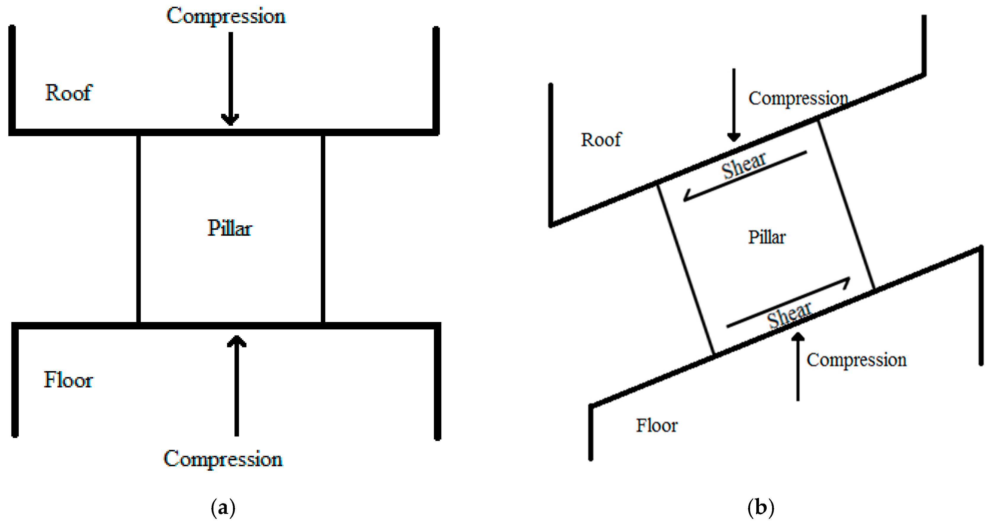
Numerical tools were used by researchers to understand the failure mechanisms and to evaluate the strength of hard-rock pillars. The elastic-brittle plastic constitutive model in finite elements and boundary element modelling packages were developed to evaluate the strength of pillars [8]. With the help of numerical modelling, the slender pillars in a limestone mine were classified as the pillars with highly variable strength, that depend on the structures which have little impact on higher width-to-height (W/H)-ratio pillars [9,10]. The failure mechanism in the slender pillars was described as brittle failure, where the failure plane passes through the centre of the pillar, while, in larger pillars, the failure mechanism was described as spalling followed by shear failure. Studies were conducted on joint spacing, joint length, and joint orientation to develop an understanding of the relationship between the area or volumetric fracture intensity and the strength of the pillars [11,12]. These studies were all based on a normal loading of the pillars, causing compression loads on them (Figure 1a).
Inclined pillars undergo oblique loading, which is a combination of compressive and shear stresses, as shown in the Figure 1b. Stress analysis studies were conducted on two pillars, one inclined along a 45° dip angle, and the other with normal loading, with the same extraction ratio. It was concluded that the failure in the dip pillar extended from one corner to the other, while the normal pillar was stable, which resulted in domino pillar bursting in Quirke mine [13]. The progressive failure of 20°-inclined pillars was described by Pritchard and Hedley at Denison mine [14]. It was described as spalling at the two sides of the pillars, followed by hour-glass fracture formation in an inclined fashion, which ultimately led to a complete failure in pillars with larger width-to-height ratios. Case studies conducted on inclined pillars and associated excavations which undergo oblique loading were described to be at higher risk of failure when compared to pillars with normal loading [15,16]. The case studies were only based on one pillar and its failure mechanism, while the strength of the pillar was not evaluated to develop pillars in an inclined fashion.
Two-dimensional finite-element numerical studies were conducted to evaluate the strength of hard-rock pillars under far-field principal stresses at different orientations, and it was concluded that the strength of the pillars with higher W/H ratios was highly affected by the orientation of the pillars [17,18]. Jessu and Spearing [19] conducted similar numerical studies to that of Suorineni [18] but with a finite difference code in a three-dimensional model to evaluate the strength and the failure mechanisms of pillars at different inclinations. It was concluded that, as the inclination increases, the pillars with higher W/H ratios have a significantly lower strength than the horizontal pillars. The study also described that the brittle failure mechanism is the dominant failure mechanism in inclined pillars, where failure starts from one corner of the pillar and proceeds to other corner. All the studies conducted were numerical modelling studies, no laboratory testing was conducted to show the effectiveness of the numerical modelling results.
This paper presents the laboratory testing of specimens under inclined loading and evaluates their reduction in strength in comparison to specimens tested under normal loading. The failure mechanisms were evaluated at the laboratory scale and were related to the cause of strength reduction. The results of the numerical modelling of pillars presented by Jessu and Spearing [19] were further evaluated to describe the strength reduction factors.
2. Materials and Test Methods
Moulded gypsum and sandstone core specimens were tested under uniaxial and oblique loading conditions. These were selected by the authors, as moulded gypsum was extensively used by many researchers [20,21] as a representative of brittle rock, and both moulded gypsum and sandstone have lower strength, which is most suitable for the currently developed testing methodology.
Gypsum specimens were prepared by mixing the gypsum powder to water with a mass ratio of 100:35. PVC tubes of 50 mm inner diameter were used to cast the specimens. The PVC tubes were cut perpendicular to the tube length to cast the normal specimens, while for inclined specimens, the PVC tubes were cut at an angle on both ends. After pouring into the moulds, the mixture was stirred to remove bubbles and then placed in an oven at a temperature of 40 °C, until the specimens’ mass reached a constant value, which was attained in three days. All specimens were created in a single batch for consistency. The surface of the normal samples was made smooth and parallel according to the International Standards of Rock Mechanics (ISRM) standards with the help of a grinder, while, for the inclined specimens, the surfaces were polished with sandpaper, first with coarse grit #60 and then with fine grit #200. Gypsum specimens with three different inclinations and four different width-to-height ratios were prepared, as shown in Figure 2a,b. Five specimens were tested in every test, therefore, a total of 60 gypsum specimens were tested.
A sandstone core of 42 mm diameter was used to conduct the test. The sandstone specimens were cut at different lengths to produce different width-to-height ratios (Figure 2c). The sample ends were prepared to be parallel and straight, as specified in the ISRM standards, with the help of a grinder. The specimens were then loaded with inclined platens at different width-to-height ratios.
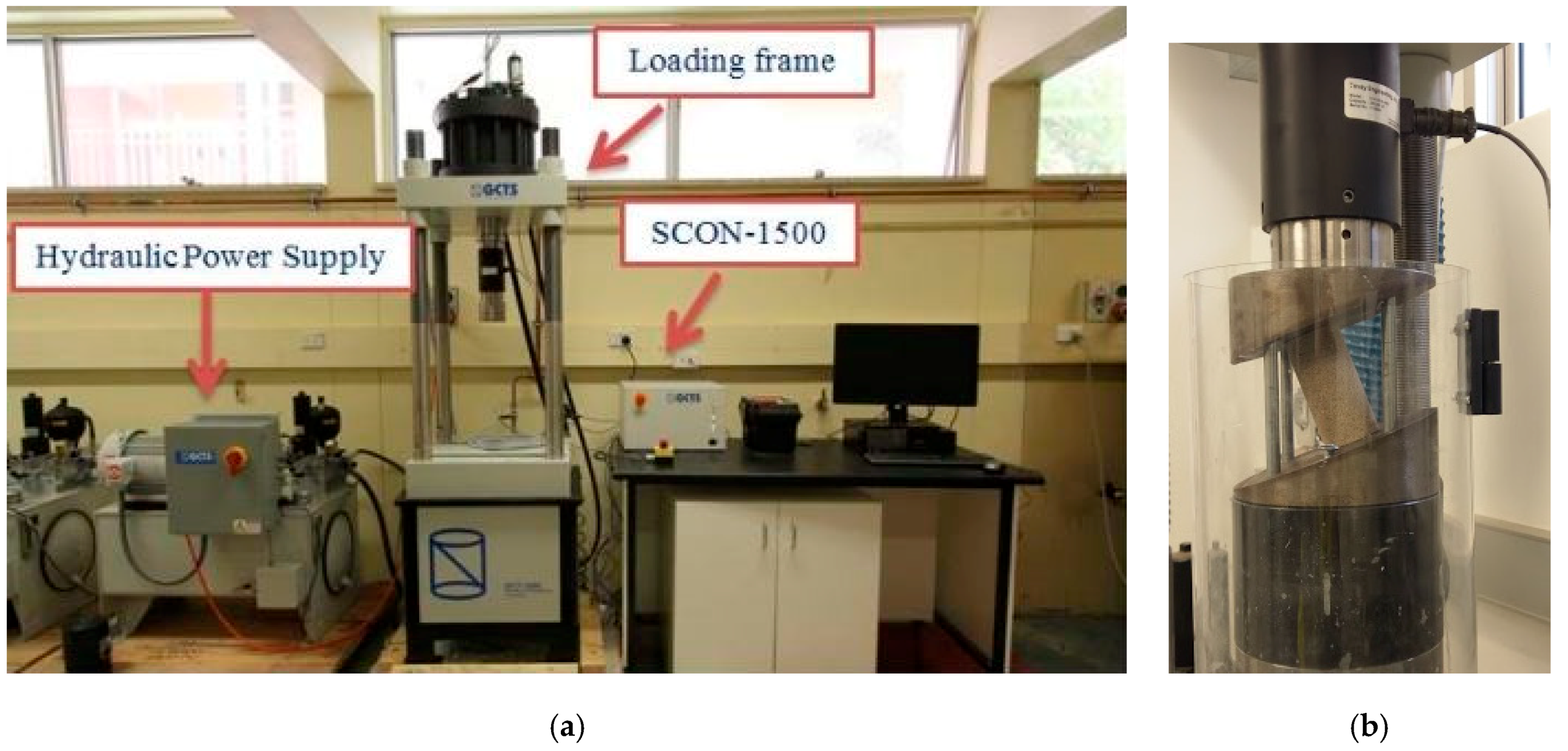
A uniaxial compression testing machine (Figure 3a), which was controlled by a servo computer program GCTS CATS 1.8 software, was used to test the gypsum and sandstone specimens in normal and inclined fashions. Straight platens were used for the uniaxial compression testing of the normal specimens, while, for the inclined specimens, platens were manufactured at 10° and 20° angles. The inclined platens were fixed to the frame of the testing machine, and then the testing of the inclined sandstones specimens was done, as shown in Figure 3b.
As the gypsum specimens were casted in the inclined fashion, they were placed directly at the centre of the straight platens, and a load of 0.2 kN was applied, such that the samples did not slip or tumble down the platens. For sandstone specimens, as they could be prepared (cut) with inclined ends, the straight specimens were placed on inclined platens in such a manner that the centre of the samples coincides with the centre point of the frame, as shown in Figure 4b. After placing the specimens on the lower platens, a load of 0.2 kN was applied to hold the samples in position.
The machine recorded load and displacement data automatically at a rate of 600 samples/minute. A displacement-type loading rate was adopted, with a fixed loading rate of 0.12 mm/min, which was in accordance with the ISRM standards, as the gypsum and sandstone specimens with length-to-diameter (L/D) ratio of 2.5 reached their peak strength in 5 to 10 min. The testing materials and the loading conditions are specified in Table 1.
Each test was conducted three or five times, and the results were averaged. Therefore, to verify if the average results were representative of the observed results, a statistical Pearson’s chi-square test was conducted for the strength values, elastic moduli, and equations proposed.
The Pearson’s chi-square test [22] is a statistical test to determine if the observed values are significantly different from the expected value. Two hypotheses are made: the null hypothesis assumes there is no significant difference between the observed values and the expected values, while the alterative hypothesis suggests there is a significant difference. The test is conducted with the help of the formula:
where is the chi-square goodness-of-fit test, O is the observed value, and E is the expected value. The degrees of freedom are determined with the help of the constraints and are one less than the number of the observed values. The chi-square and degrees of freedom are evaluated, and the probability is determined with the help of tables. If the probability is less than the significance level, which is generally taken as 0.05 or 0.1, then the null hypothesis is rejected. This shows that the expected value is significantly different when compared to the observed value.
Chi-square goodness of fit was used in this paper to determine if the average values were representative of the observed values. The chi-square values and the degrees of freedom are for all the tests conducted. The probability or the p-value is determined to show the non-significant difference between the observed values and the average values.
3. Results
3.1. Material Properties of the Two Different Rock Types
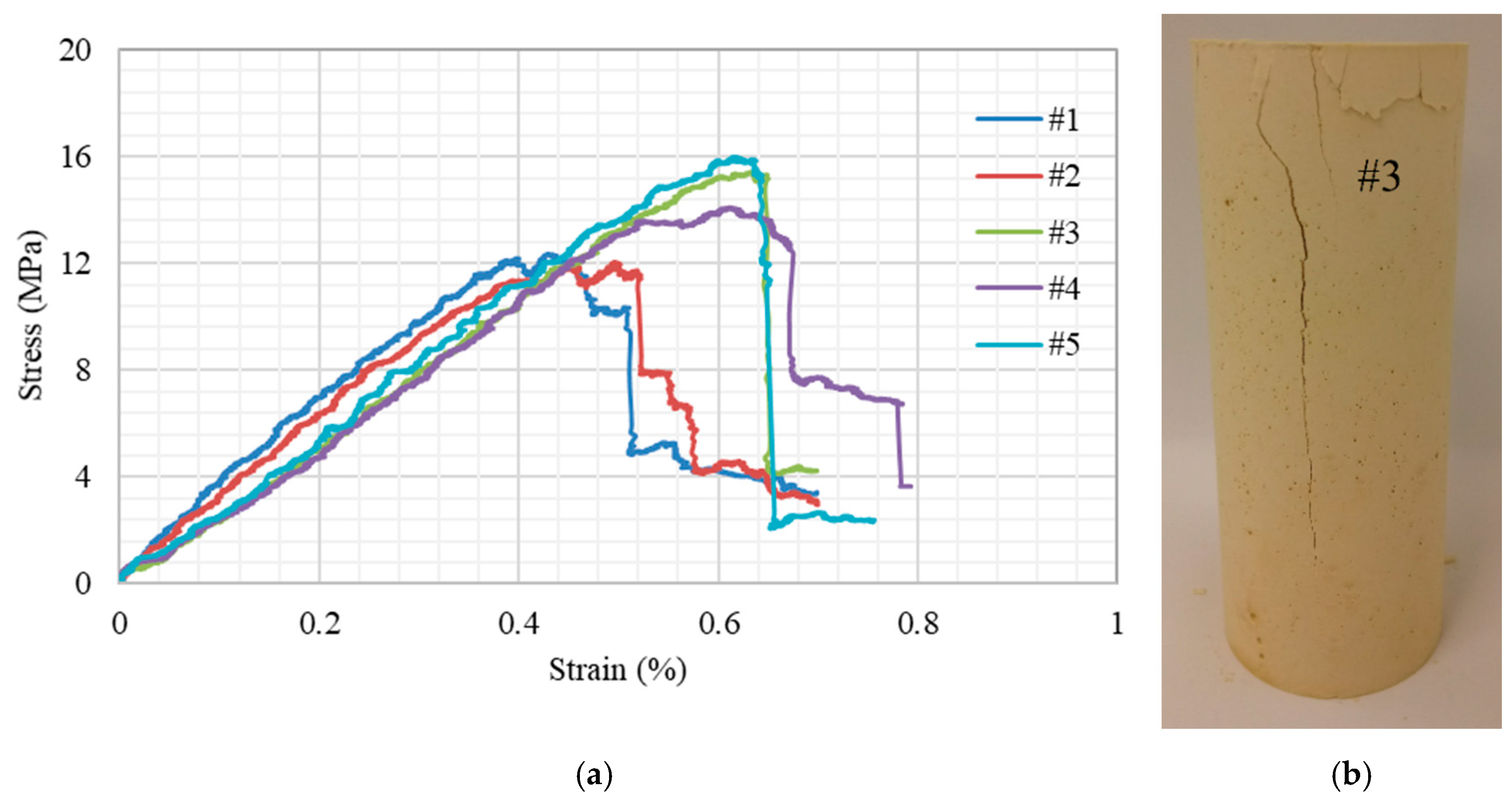
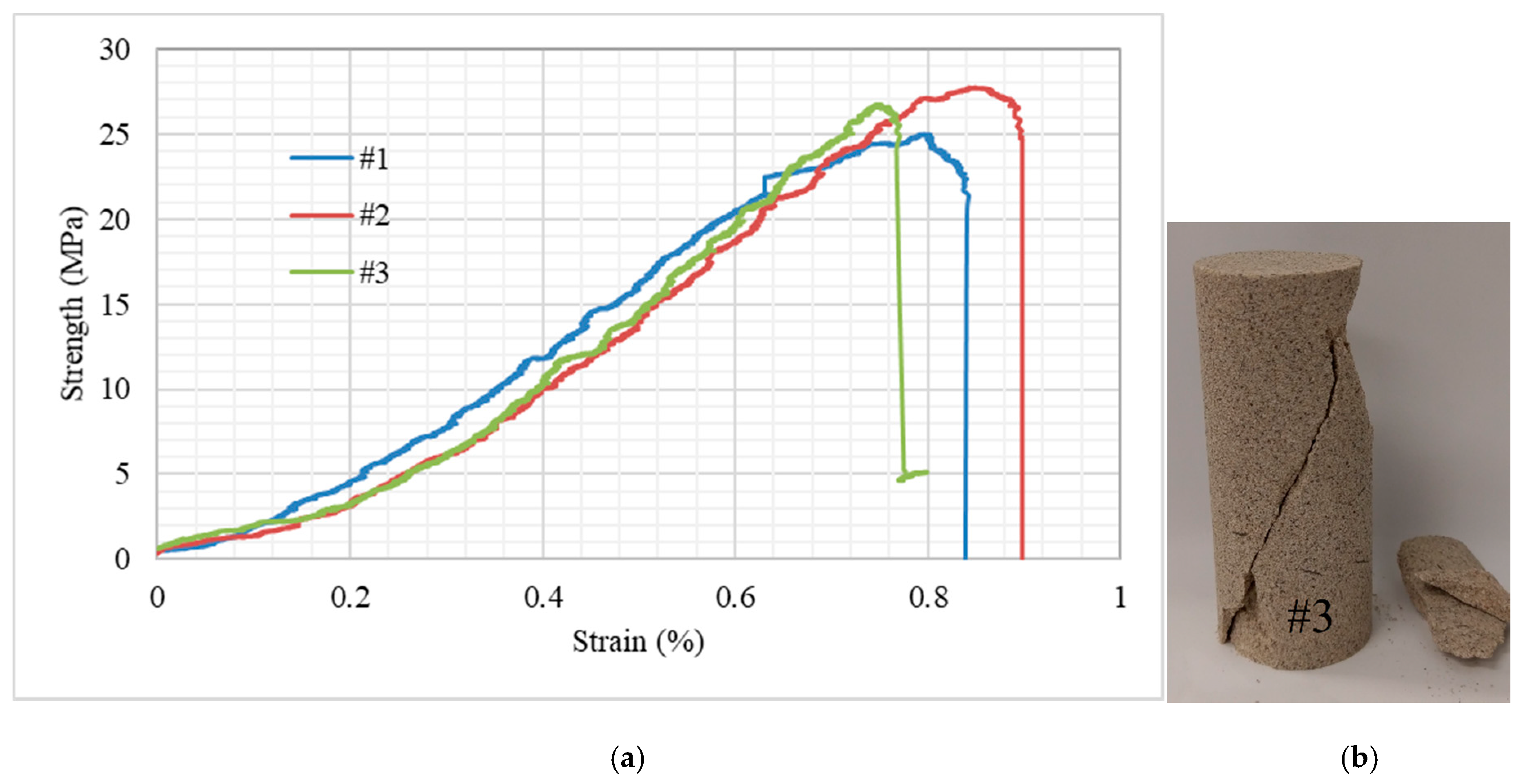
Initially, the uniaxial compressive strength and elastic modulus of the moulded gypsum and the sandstone were determined by preparing the specimens with a length-to-diameter (L/D) ratio of 2.5, as per the ISRM standards. The gypsum moulds and the sandstone specimens had a diameter of 50 mm and 42 mm, and lengths of about 125 mm and 105 mm, respectively. Five specimens were tested for moulded gypsum and three specimens for sandstone, for consistency. The stress–strain graphs of the gypsum and the sandstone specimens are shown in Figure 4a and Figure 5a. The failure modes were found to be axial splitting in the gypsum samples and single-shear plane failure in the sandstone samples, as shown in Figure 4b and Figure 5b.
The average uniaxial strength and the average elastic modulus of the moulded gypsum and sandstone with their standard deviations are shown in Table 2. The standard deviations were less than 10% for the uniaxial compressive strength and elastic modulus for both the specimens. The goodness-of-fit statistical test (chi-square test) was conducted on the specimens to understand if the average strength and average elastic modulus appropriately represented the sample strength and elastic modulus. A p-value greater than 0.05 in the goodness-of-fit test suggested that the difference between the sample strength and the average strength was not significant. Therefore, the average strength and the average elastic modulus were representative of the strength and the elastic modulus of all specimens.
3.2. Strength of Gypsum and Sandstone Specimens at Different Inclinations
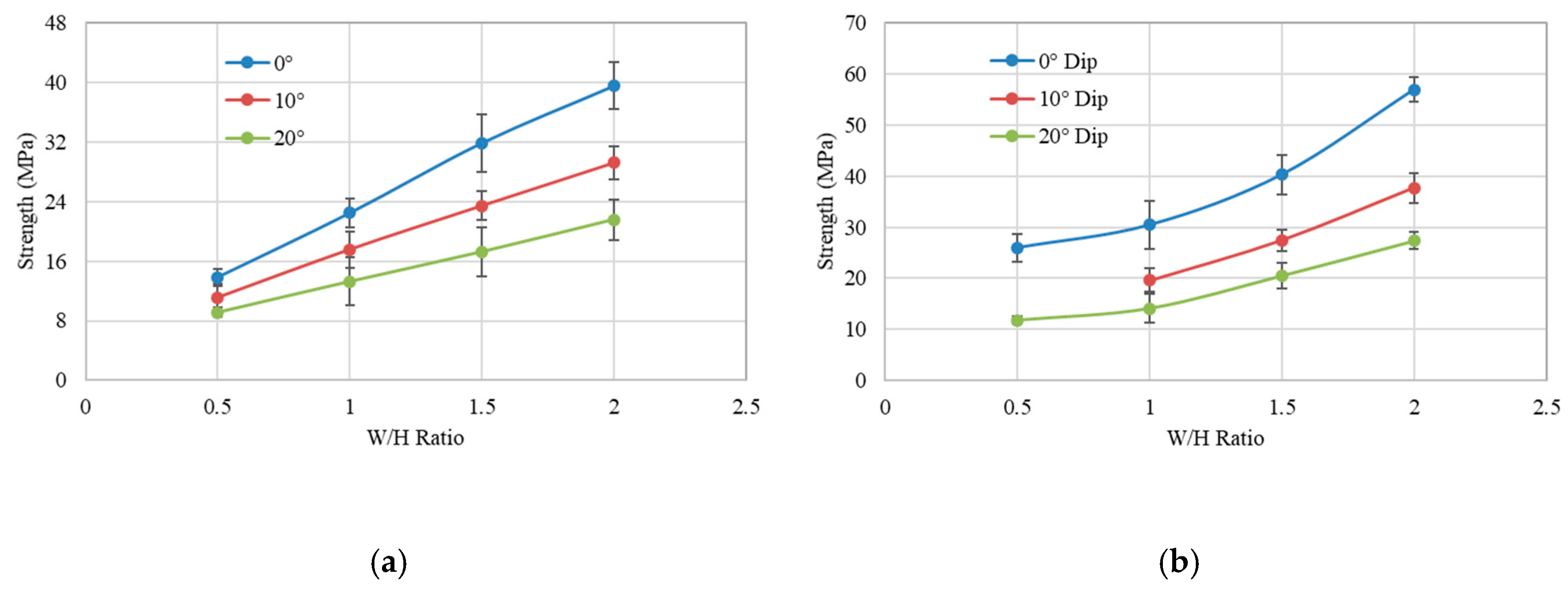
Moulded gypsum and sandstone were tested with four different width-to-height ratios of 0.5, 1.0, 1.5, and 2.0. The heights of the specimens were varied to attain the desired width to height ratios. Specimens with inclination of 0°, 10°, and 20° were tested to evaluate their strength and understand the failure mechanisms at different width-to-height ratios.
Figure 6 shows the strength of the specimens at different inclinations, indicating less than 10% standard deviation in all specimens. It can be observed that the strength of the specimens positively corresponded to their width-to-height ratios, and the rate of the increase decreased with inclination. It can be observed that the strength reduction due to inclination was higher in specimens with larger W/H ratios than in those with smaller W/H ratios.
3.3. Failure Mechanism of Gypsum Specimens at Different Inclinations
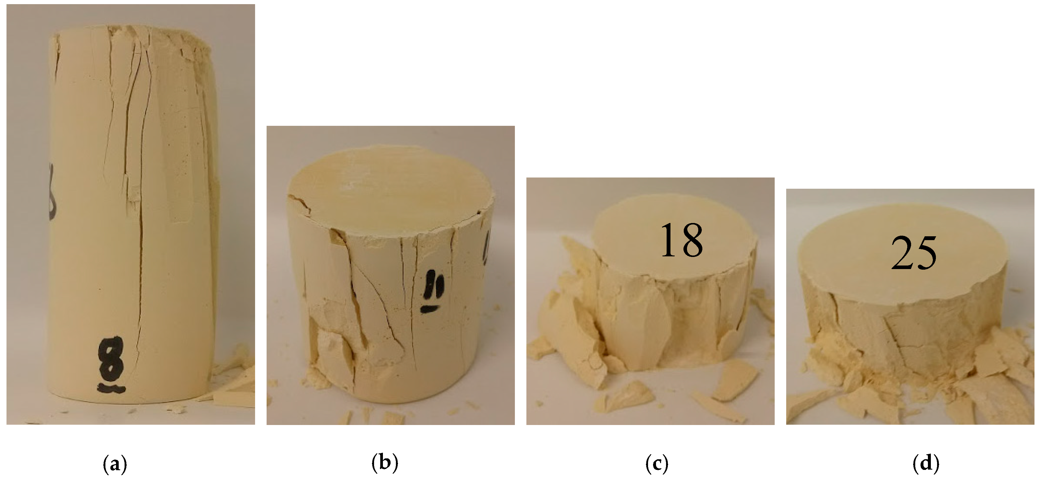
The failure mechanisms of the gypsum specimens in the normal loading conditions are shown in Figure 7. The axial splitting failure was dominant in the specimens with a W/H ratio of 0.5 and also passed through the centre of the sample. The sample strength reached a peak and dropped down rapidly because of the failure of the sample from the centre of the pillar. In larger specimens, where the W/H ratio was greater than 1.0, the failure was observed to be spalling on the sides, which caused a reduction in size of the specimens and the hour-glass formation. Therefore, this was similar to the failure mechanism observed in underground mine pillars, whereby the slender pillars failed through the centre of the pillar, and the larger pillars failed through gradual spalling on the sides and then hourglass formation, which led to complete failure [23].
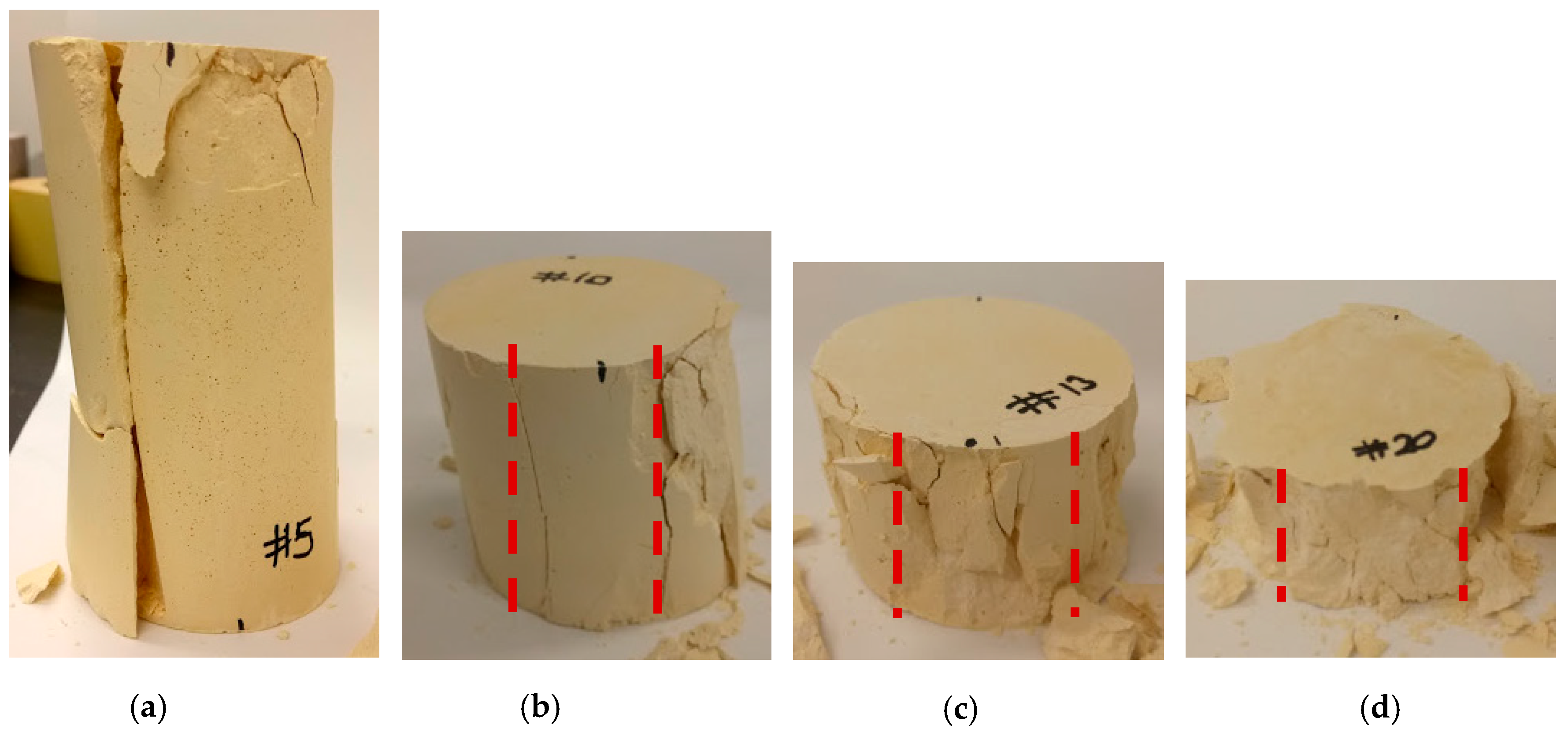
The failure mechanisms of the 10° specimens are shown in Figure 8. The failure of the sample with a W/H ratio of 0.5 was observed to be axial splitting, which was similar to the failure of the sample in normal loading condition. The failure was observed to be passing through the centre of the sample (Figure 8a), and the strength dropped rapidly as it reached the peak. In larger specimens, the failure was majorly concentrated on the skin of the specimens, particularly, at two corners, as shown in Figure 8b–d. Comparing Figure 8b,d, the area affected by the failure was higher for a W/H ratio of 1.0 and decreased with the increase of the W/H ratio. This showed that the load-bearing surface was higher for a W/H ratio of 2.0; therefore, the strength of the specimens increased with the increase of the W/H ratio.
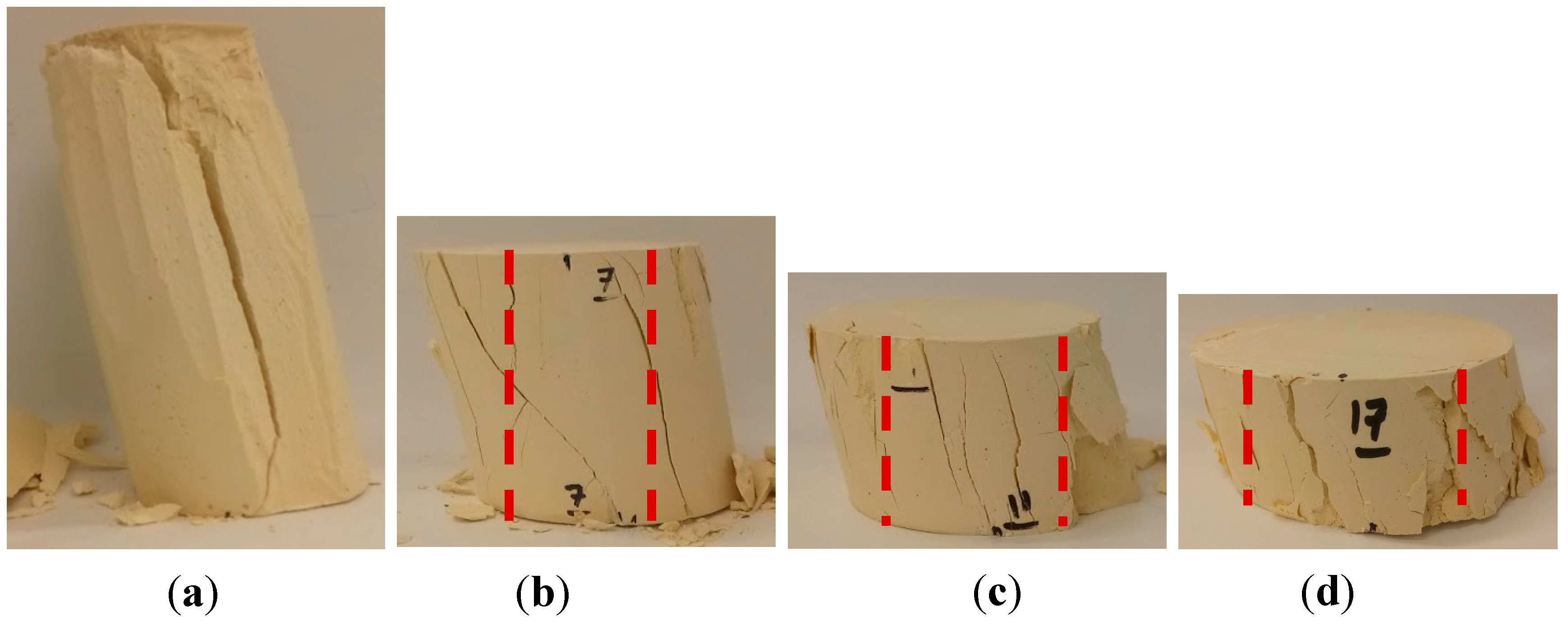
The failure of the 20°-inclined specimens (Figure 9) was similar to that of the 10°-inclined specimens, and the failure of specimens with a W/H ratio of 0.5 was due to axial splitting and passed through the centre of the samples (Figure 9a). In larger specimens, the stress concentration was higher at the two corners, and breakage was mostly observed in these two corners, as shown in Figure 9b–d.
4. Numerical Modelling
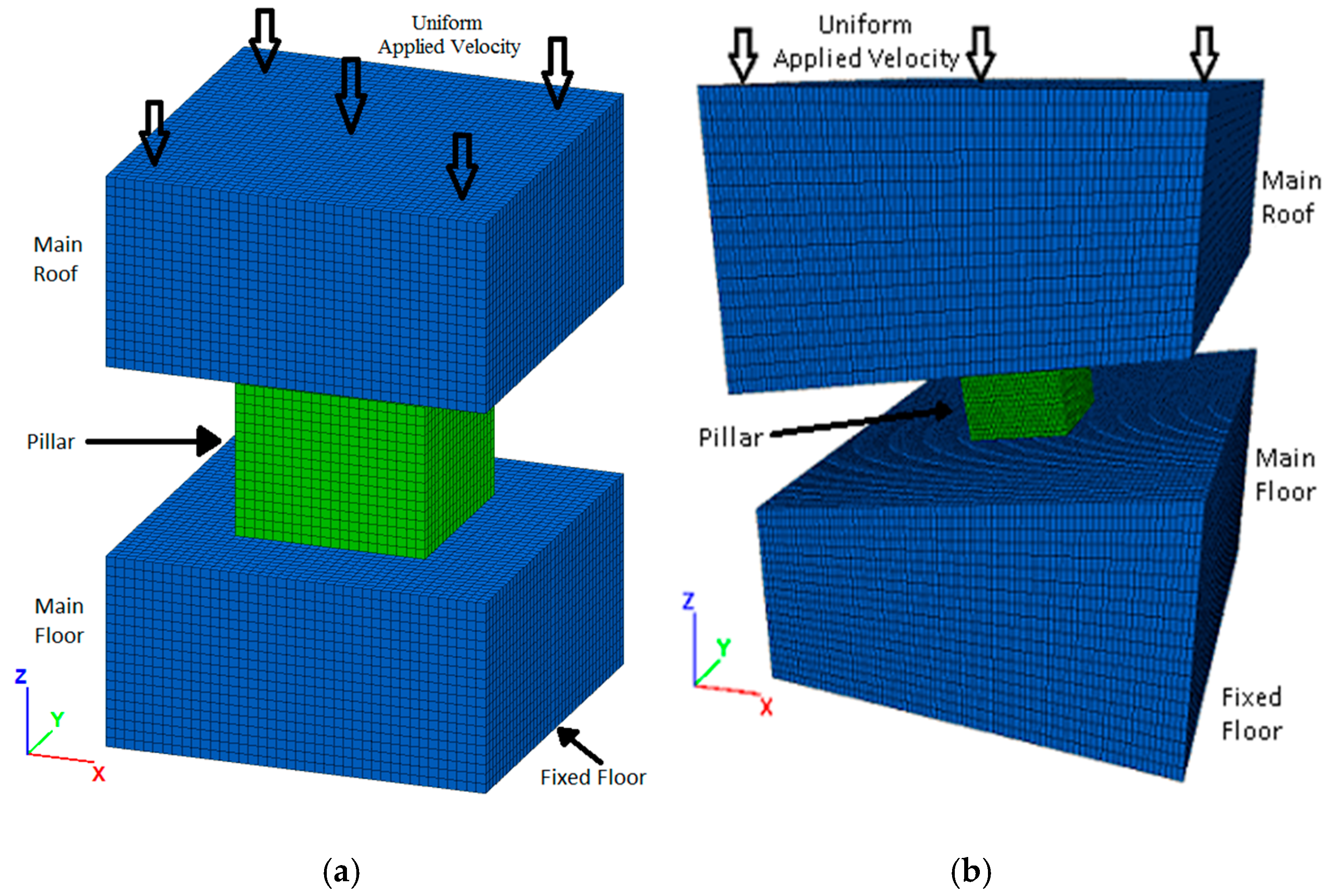
FLAC3D [24], a geotechnical finite difference modelling package, was used to simulate the pillars, as shown in Figure 10. A three-dimensional co-ordinate system was used, where the horizontal plane was represented in the x and y directions, and the vertical plane was represented in z-direction. For the inclined pillars, inclination was measured from the x direction, as shown in Figure 10b. The model consists of the main floor, the main roof, and the pillar with a height of 4 m, considering the Lunder and Pakalnis database [3]. The width of the pillars was varied to achieve the width-to-height ratio of the pillars. The extraction ratio was kept constant for all the vertical pillars at 75% and for the inclined pillars, the boundaries were established far enough to avoid boundary effects on the performance of the inclined pillars and their failure behaviour. The thickness of the roof and the floor was maintained at three times the pillar height in all models to avoid the boundary effects.
Boundary conditions such as fixed supports were placed at the bottom of the floor, which restricted the displacement and velocity in both parallel and normal directions. Roller supports were placed on the sides, thus restricting the velocity and displacement in the normal direction. Loading was applied in the form of uniform velocity on the top of the roof until the pillar entirely failed and the residual strength reached 50% of the peak strength, as recommended by Lorig and Cabrera [25].
The bilinear strain hardening–softening ubiquitous joint constitutive model was applied to simulate the pillars. This model is based on the Mohr Coulomb strength criterion and the strain softening or hardening as a function of the deviatoric plastic strain [24]. The elastic criterion was applied to simulate the roof and floor to ensure that the roof and floor were stronger than the pillar and failure was only induced in the pillar. The model properties are summarized in Table 3 and Table 4 [26].
The critical parameter in defining the strain-softening properties is the model element size. The element size used was 0.5 m × 0.5 m × 0.5 m throughout the model, and cohesion softening was carried out to calibrate the horizontal the pillar results to those of Lunder and Paklnis [3]. The horizontal pillars were simulated at four different width-to-height ratios (0.5, 1.0, 1.5, and 2.0). The numerical model results were found to be in the range of 2% of the theoretical results, as shown in Figure 11a.
Jessu and Spearing [19] simulated pillars at five different inclinations of 0°, 10°, 20°, 30°, and 40° with four different width-to-height ratios. It was concluded that the pillar strength increased with the increase of the width-to-height ratio at all the inclinations of the pillars, as shown in Figure 11. The results presented in Jessu and Spearing [19] for the numerical modelling of horizontal and inclined pillars were analysed further to determine the strength reduction factors.
5. Discussion
5.1. Evaluating Strength Reduction Factors with Laboratory and Numerical Methods
As the strength of the inclined specimens were found to be lower than that of the horizontal specimens, the ratio of the strength of the inclined specimens to the strength of the horizontal specimens was determined.
5.1.1. Strength Reduction Factors for Gypsum Specimens and Sandstone Specimens
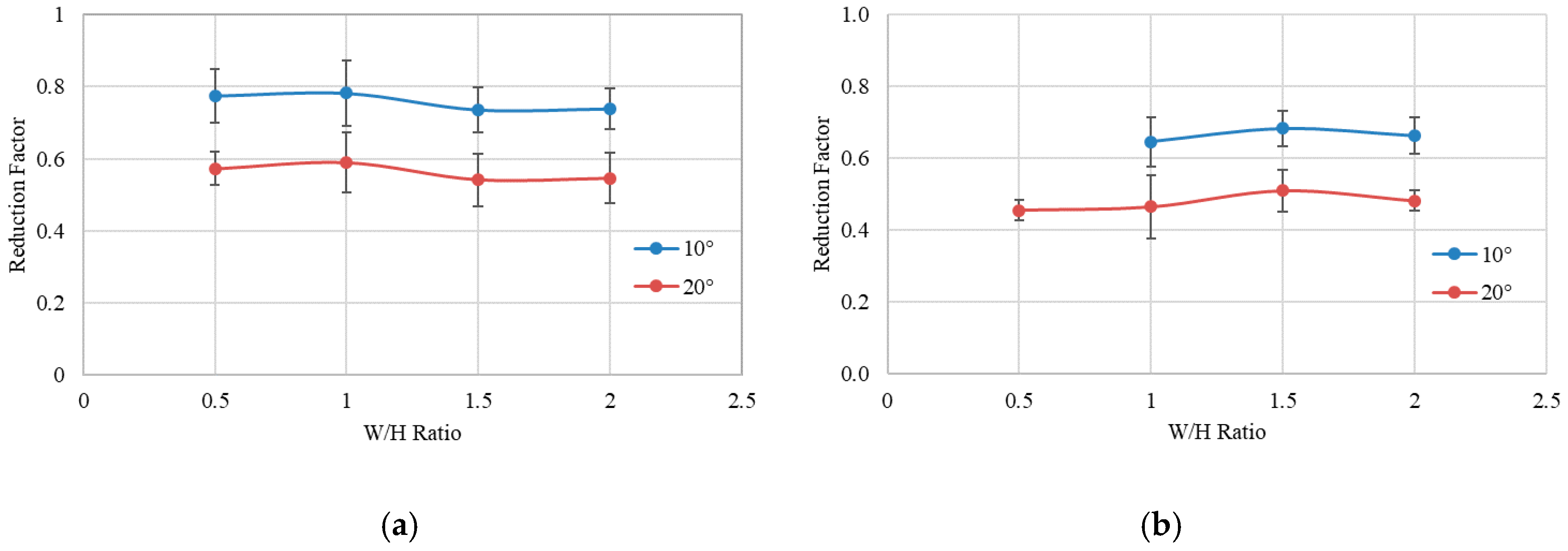
It was found that, at a specific inclination, the percentage reduction in the strength of the specimens for all the width-to height-ratios was similar, as shown in Figure 12. At 10° inclination, the strength of the gypsum specimens was found to be about 76–79% of that of the normal specimens and, at 20° inclination, about 54–59% of that of the normal specimens. In sandstone specimens, it was found that the strength of the 10°-inclined specimens was 67–72% of that of the normal specimens, while the strength of the 20°-inclines specimens was about 42–47% of that of the normal specimens. Therefore, a reduction factor could be developed to determine the strength of the inclined specimens with respect to the strength of the normal specimens.
The average reduction factors were determined for 10°- and 20°-inclined gypsum specimens as 78% and 56%, respectively, while, for the 10°- and 20°-inclined sandstone specimens as 71% and 43%, respectively, as shown in Table 3. The goodness-of-fit test was conducted to determine if these factors were representative for all the specimens. The p-value was evaluated (Table 5) and found to be greater than 0.05, which showed that the difference between the reduction factor for individual specimens and the average reduction factor was not significant. Therefore, the average reduction factor can be adopted to consider the effect of inclination on the specimens across all the width-to-height ratios.
5.1.2. Strength Reduction Factors for Numerically Simulated Pillars
In the laboratory-based results of gypsum and sandstone, the values of the strength of the inclined specimens to the strength of the normal specimens at all the W/H ratios were consistent. The laboratory results showed that the strength reduction factors can be used to predict the strength of the inclined specimens at any width-to-height ratios. The laboratory test results are the basis for understanding the strength of the large-scale pillars [27,28]. Therefore, as the strength reduction factors are consistent throughout all the W/H ratios for a specific inclination in the laboratory specimens, the strength reduction factors should be consistent throughout all the W/H ratios in large-scale pillars.
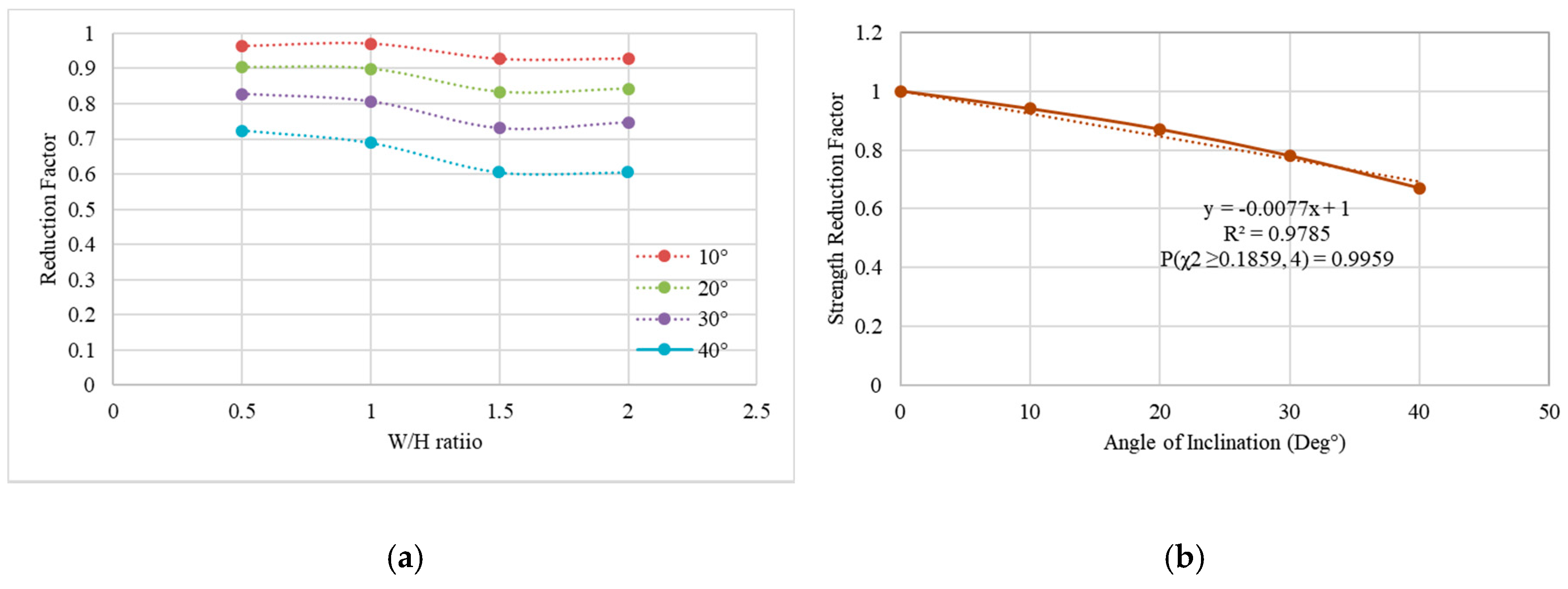
The strength reduction factors were evaluated by comparing the strength of the inclined pillars to that of the normal pillars, as shown in Figure 13a. The strength reduction factors were found to be slightly higher for smaller W/H ratios than for larger W/H ratios. For 10°-inclined pillars, the reduction factors ranged from 0.92 to 0.97. Similarly, for 20°-, 30°-, and 40°-inclined pillars, the ranges of the strength reduction factors were found to be 0.83–0.90, 0.73–0.83, 0.61–0.72, respectively.
The average of these strength reduction factors was evaluated and is shown in Table 6. The goodness-of-fit test was conducted to understand if the average was representative of all pillar width-to-height ratios at a certain inclination of the pillar. The p-values from the chi-square test (Table 6) were found be higher than 0.05, which effectively explained that the difference between the average reduction factor and the individual reduction factor was not significant. Therefore, the average strength reduction factors can be utilized to represent all the-width-to-height ratios.
The laboratory test results for the inclined pillars were compared to the numerical test results of pillars at 10° and 20° inclinations, as shown in Table 7. For sandstone, it was found that it had higher reduction in strength when compared to gypsum, which can be attributed to the scale of the samples (i.e., the diameter of the gypsum samples was higher than that of the sandstone samples). Similarly, as the numerically simulated pillars were very large when compared to the laboratory samples, the reduction in strength of the pillars was less, as shown in Table 7.
For large-scale pillars, the numerical models were simulated and calibrated according to Lunder and Pakalnis [3]. It was found that the strength reduction factors were consistent throughout all the width-to-height ratios for any inclination. To account for inclination in the empirical approach developed by Lunder and Pakalnis [3], a relationship between the inclination and the reduction factor was developed.
A linear relationship was developed between the average strength reduction factors (RF) and the inclination of the pillar (θ), as shown in Figure 13b. The equation can be written as:
5.2. Failure Mechanism of the Inclined Specimens and Pillars
The failure mechanism of the inclined specimens was different from that of the horizontal specimens, as shown in Figure 7, Figure 8 and Figure 9. In the inclined specimens, the failure was mostly concentrated at the two corners of the specimens towards the sample dip. To understand the strength loss in the inclined specimens, a theoretical method was developed based on the areal or volumetric failure of the specimens (pillars).
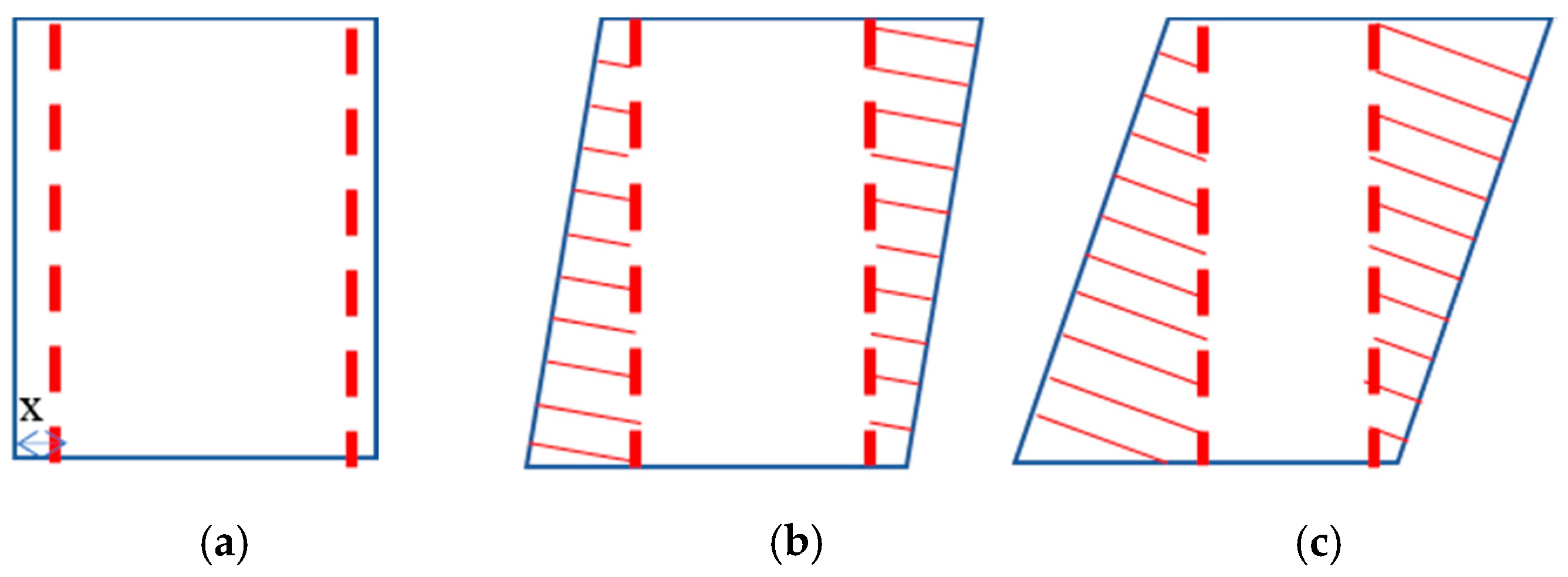
In Figure 14, the red dotted lines show the breakage of the skin of the specimens, and the shaded area shows the affected corners. In 10°-inclined specimens, the area of the affected corners was smaller than that of the 20°-inclined specimens. In a two-dimensional space, the area affected can be estimated by rectangular and triangular areas which are mainly dependent on the angle of inclination (θ) and the height of the sample (H).
In normal conditions, if x is the affected skin width, then the affected area () can be determined as the area of a rectangle, such as:
In inclined conditions, the affected area () can be estimated considering the areas of a rectangle and a triangle, such as:
The ratio between the affected area in inclined loading conditions and in normal loading condition is dependent on the angle of inclination (θ), which is determined by:
where ) is dependent on the sample in normal loading conditions and is represented as a constant ‘K’. Therefore, the ratio is directly proportional to the angle of inclination of the pillar ().
Strength loss in the inclined specimens compared to the normal specimens was determined in gypsum and sandstone specimens, as shown in Table 8. The proportionality constant was determined between the strength loss and the angle of inclination of the sample. The proportionality constant was found to be similar for both inclinations. Therefore, strength loss is also directly proportional to the inclination of the sample. As the strength loss and the ratio of the failure area are both directly proportional to the inclination of the sample, it can be concluded that failure at the corners of the inclined specimens leads to loss of strength when compared to the normal specimens.
Similar to the laboratory tests, the loss of strength was evaluated for all the numerically simulated inclined pillars and was found to be approximately 34–39 times the inclination of the pillars, as shown in Table 9. This indicated that the strength loss was directly proportional to the inclination of the pillar and, therefore, could be attributed to the failure of the corners of the pillars.
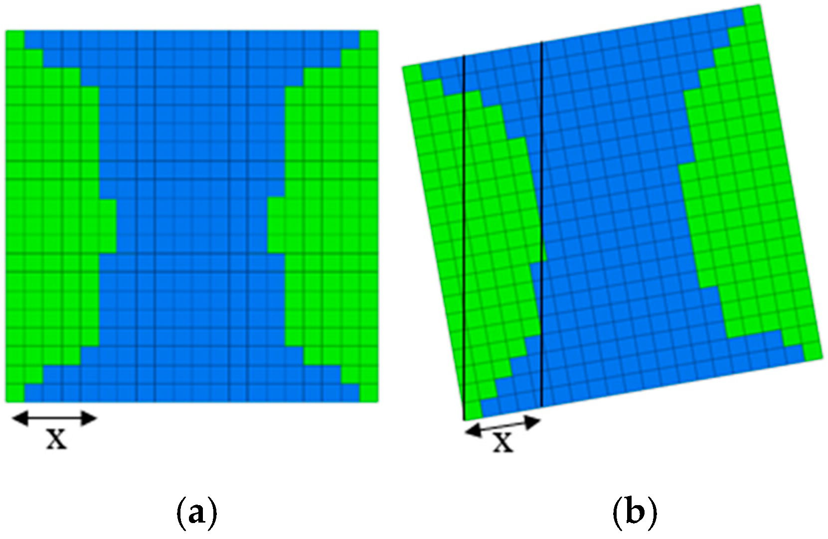
As the failure in the numerical models can be interpreted, volumetric analysis of the elastic and yielded zones was carried out to develop a relationship between the strength loss and the volume affected in inclined pillars with respect to the volume affected in horizontal pillars. The failure in the horizontal and inclined pillars at the peak strength with a W/H ratio of 1.0 is shown in Figure 15. The affected skin width was determined between 1 and 1.25 m for a W/H ratio of 1.0 in both horizontal and inclined pillars. The volume was estimated for the yielded zones in the horizontal pillar and inclined pillar, and the ratio was determined for all the inclined pillars, as shown in Table 9. It was found that the volumetric ratio of the failure region of the inclined pillars (Table 9) was twice the strength loss across all the inclinations. Therefore, the strength loss in the inclined pillars could be mostly attributed to the failure of the corners.
5.3. Example of the Use of Strength Reduction Factors for Inclined Pillar Design
Let us assume that the pillar stress was 55 MPa with an extraction ratio of 0.75. If the safety factor used to design the pillars is taken as 1.4, then the design of the pillar should be such that it has a strength of 77 MPa. Let us assume that the uniaxial compressive strength of the rock is about 150 MPa, then with the help of the Lunder and Pakalnis approach [3], the width-to-height ratio needed to design a horizontal pillar having a strength of 77 MPa is 1.5.
For 20° inclination, maintaining the same conditions, if a pillar with a W/H ratio of 1.5 is designed, the safety factor is reduced by a factor of 0.87, as the actual strength of the 20°-inclined pillar is 0.94 times that of the horizontal pillar. Therefore, the safety factor for a 20°-inclined pillar turns out to be 1.2, and the design could be considered reasonably good. If the safety factors are to be maintained at 1.4, the W/H ratio needed to design a 20°-inclined pillar can be evaluated by including 0.87 as the reduction factor in the Lunder and Pakalnis [3] approach and results to be 1.9. Therefore, the strength reduction factors can be better used to design inclined pillars with reasonably good safety factors.
6. Conclusions
On the basis of the laboratory and numerical results, the following conclusions are drawn:
- Strength reduction factors of 0.78 and 0.56 for 10°- and 20°-inclined gypsum pillars and 0.71 and 0.43 for 10°- and 20°-inclined sandstone specimens are consistent throughout all the width-to-height ratios at a specific sample inclination. Therefore, average strength reduction factors can be utilized for designing inclined pillars with respect to horizontal pillars.
- Horizontal pillars were calibrated using the Lunder and Pakalnis database [3]. The average strength reduction factors obtained from numerical modelling were 0.94 for 10° inclination, 0.87 for 20° inclination, 0.78 for 30° inclination, and 0.67 for 40° inclination. These reductions factors can be used in an empirical approach (Equation 2) to evaluate the strength of the inclined pillars.
- With the numerical modelling, an equation is proposed for strength reduction factors with respect to their inclinations.
- Reduction factors will lead to a better design of inclined pillars, with adequate safety factors.
- In larger pillars, the failure at the corners of the inclined pillars leads to excessive loss of strength compared to horizontal pillars.
Author Contributions
Conceptualization, K.V.J.; Methodology, K.V.J.; Software, K.V.J.; Validation, K.V.J.; Formal Analysis, K.V.J.; Investigation, K.V.J.; Resources, A.J.S.S.; Writing-Original Draft Preparation, K.V.J.; Writing-Review & Editing, A.J.S.S. and M.S.; Supervision, A.J.S.S.
Funding
This research received no external funding.
Conflicts of Interest
The authors declare no conflict of interest.
References
- Salamon, M.D.G.; Munro, A.H. A study of the strength of coal pillars. J. S. Afr. Inst. Min. Metall. 1967, 68, 55–67. [Google Scholar]
- Hedley, D.G.F.; Grant, F. Stope-and-pillar design for the Elliot Lake Uranium Mines. Bull. Can. Inst. Min. Metall. 1972, 65, 37–44. [Google Scholar]
- Lunder, P.J.; Pakalnis, R. Determination of the strength of hard rock mine pillars. Bull. Can. Inst. Min. Metall. 1997, 90, 51–55. [Google Scholar]
- Kimmelmann, M.R.; Hyde, B.; Madgwick, R.J. The use of computer applications at BCL Limited in planning pillar extraction and design of mining layouts. In Proceedings of the ISRM Symposium: Design and Performance of Underground Excavations, London, UK, 3–6 September 1984; pp. 53–63. [Google Scholar]
- Krauland, N.; Soder, P.E. Determining pillar strength from pillar failure observations. Eng. Min. J. 1987, 8, 34–40. [Google Scholar]
- Potvin, Y.; Hudyma, M.; Miller, H.D.S. Rib pillar design in open stope mining. Bull. Can. Inst. Min. Metall. 1989, 82, 31–36. [Google Scholar]
- Sjoberg, J.S. Failure modes and pillar behaviour in the Zinkgruvan mine. In Proceedings of the 33rd U.S. Rock Mechanics Symposium; Tillerson, J.A., Wawersik, W.R., Eds.; A.A. Balkema: Sante Fe, NM, USA; Rotterdam, The Netherlands, 1992; pp. 491–500. [Google Scholar]
- Martin, C.D.; Maybee, W.G. The strength of hard-rock pillars. Int. J. Rock Mech. Min. Sci. 2000, 37, 1239–1246. [Google Scholar] [CrossRef]
- Esterhuizen, G.S. An evaluation of the strength of slender pillars. In Transactions of Society for Mining, Metallurgy, and Exploration, Inc. Vol. 320; Society for Mining, Metallurgy, and Exploration, Inc.: Littleton, CO, USA, 2006; pp. 69–76. [Google Scholar]
- Esterhuizen, G.S.; Dolinar, D.R.; Ellenberger, J.L. Pillar strength and design methodology for stone mines. In Proceedings of the 27th International Conference on Ground Control in Mining, Morgantown, WV, USA, 29–31 July 2008; pp. 241–253. [Google Scholar]
- Elmo, D.; Stead, D. An integrated numerical modelling–discrete fracture network approach applied to the characterisation of rock mass strength of naturally fractured pillars. Rock Mech. Rock Eng. 2010, 43, 3–19. [Google Scholar] [CrossRef]
- Zhang, Y. Modelling Hard Rock Pillars Using a Synthetic Rock Mass Approach. Ph.D. Thesis, Simon Fraser University, Burnaby, BC, Canada, 2014. [Google Scholar]
- Hedley, D.G.F.; Roxburgh, J.W.; Muppalaneni, S.N. A case history of rockbursts at Elliot Lake. In Proceedings of Second International Conference on Stability in Underground Mining; Brawner, C.O., Ed.; American Institute of Mining, Metallurgical and Petroleum Engineers Inc.: New York, NY, USA, 1984; pp. 210–234. [Google Scholar]
- Pritchard, C.J.; Hedley, D.G.F. Progressive pillar failure and rockbursting at Denison Mine. In Rockbursts and Seismicity in Mines, Young (ed.); Baikema: Rotterdam, The Netherlands, 1993. [Google Scholar]
- Kvapil, R.L.; Beaza, J.R.; Flores, G. Block caving at EI Teniente mine, Chile. Trans. Inst. Min. Metall. A-Min. Ind. 1989, 98, A43–A56. [Google Scholar]
- Whyatt, J.; Varley, F. Catastrophic failures of underground evaporite mines. In Proceedings of the Twenty-Seventh International Conference on Ground Control in Mining, Morgantown, WV, USA, 29–31 July 2008; pp. 113–122. [Google Scholar]
- Suorineni, F.T.; Mgumbwa, J.J.; Kaiser, P.K.; Thibodeau, D. Mining of orebodies under shear loading Part 1—Case histories. Min. Technol. Trans. Inst. Min. Metall. A 2011, 120, 138–147. [Google Scholar] [CrossRef]
- Suorineni, F.T.; Mgumbwa, J.J.; Kaiser, P.K.; Thibodeau, D. Mining of orebodies under shear loading Part 2—Failure modes and mechanisms. Min. Technol. Trans. Inst. Min. Metall. A 2014, 123, 240–249. [Google Scholar] [CrossRef]
- Jessu, K.V.; Spearing, A.J.S. Effect of Dip on Pillar Strength. South Afr. Inst. Min. Metall. 2018, 118, 765–776. [Google Scholar] [CrossRef]
- Bobet, A.; Einstein, H.H. Fracture coalescence in rock-type materials under uniaxial and biaxial compression. Int. J. Rock Mech. Min. Sci. 1998, 35, 863–888. [Google Scholar] [CrossRef]
- Wong, L.; Einstein, H. Crack Coalescence in Molded Gypsum and Carrara Marble: Part 2—Microscopic Observations and Interpretation. Rock Mech. Rock Eng. 2009, 42, 513–545. [Google Scholar] [CrossRef]
- Pearson, K. On the criterion that a given system of deviations from the probable in the case of a correlated system of variables is such that it can be reasonably supposed to have arisen from random sampling. Philos. Mag. Ser. 5 1900, 50, 157–175. [Google Scholar] [CrossRef]
- Roberts, D.P.; Tolfree, D.; McIntire, H. Using confinement as a means to estimate pillar strength in a room and pillar mine. In Proceedings of the 1st Canada-US Rock Mechanics Symposium, Vancouver, BC, Canada, 27–31 May 2007; pp. 1455–1462. [Google Scholar]
- Itasca Consulting Group. Fast Lagrangian Analysis of Continua in 3Dimensions; Itasca Consulting Group: Minneapolis, MN, USA, 2018. [Google Scholar]
- Lorig, L.J.; Cabrera, A. Pillar Strength Estimates for Foliated and Inclined Pillars in Schistose Material. In Proceedings of the 3rd International FLAC/DEM Symposium, Hangzhou, China, 22–24 October 2013; Paper: 01-01. Zhu, H., Ed.; Itasca International Inc.: Minneapolis, MN, USA, 2013. [Google Scholar]
- Dolinar, D.R.; Esterhuizen, G.S. Evaluation of the effects of length on strength of slender pillars in limestone mines using numerical modelling. In Proceedings of the 26th International Conference on Ground Control in Mining, Morgantown, WV, USA, 31 July–2 August 2007; West Virginia University: Morgantown, WV, USA; pp. 304–313. [Google Scholar]
- Ayres da Silva, L.A.; Ayres da Silva, A.L.M.; Sansone, E.C. The shape effect and rock mass structural control for mine pillar design. In EUROCK 2013: Rock Mechanics for Resources, Energy and Environment; CRC Press/Balkema: London, UK; pp. 563–567.
- Ayres da Silva, L.A.; Ayres da Silva, A.L.M. The interaction between the scale effect and the shape effect in the mine pillar design. In Proceedings of the ISRM Regional Symposium—EUROCK, Vigo, Spain, 27–29 May 2014; pp. 683–687. [Google Scholar]
Figure 1.
(a) Normal loading on pillars, (b) oblique loading on pillars.

Figure 2.
(a) 0° Gypsum specimens, (b) 10°-inclined gypsum specimens, (c) sandstone specimen.

Figure 3.
(a) Uniaxial compression testing machine, (b) modified platens for inclined pillar testing.
Figure 3.
(a) Uniaxial compression testing machine, (b) modified platens for inclined pillar testing.

Figure 4.
(a) Stress–strain behaviour of the moulded gypsum in the uniaxial compressive strength (UCS) test, (b) axial splitting failure mechanism of the moulded gypsum in the UCS test.
Figure 4.
(a) Stress–strain behaviour of the moulded gypsum in the uniaxial compressive strength (UCS) test, (b) axial splitting failure mechanism of the moulded gypsum in the UCS test.

Figure 5.
(a) Stress–Strain behaviour of the sandstone in the UCS test, (b) shear failure mechanism of the sandstone in the UCS test.
Figure 5.
(a) Stress–Strain behaviour of the sandstone in the UCS test, (b) shear failure mechanism of the sandstone in the UCS test.

Figure 6.
Strength variation of the (a) moulded gypsum specimens, (b) sandstone specimens with respect to their W/H ratio at different inclinations.
Figure 6.
Strength variation of the (a) moulded gypsum specimens, (b) sandstone specimens with respect to their W/H ratio at different inclinations.

Figure 7.
Failure mechanisms of the gypsum specimens under normal loading conditions: (a) W/H ratio of 0.5, (b) W/H ratio of 1.0, (c) W/H ratio of 1.5, (d) W/H ratio of 2.0.
Figure 7.
Failure mechanisms of the gypsum specimens under normal loading conditions: (a) W/H ratio of 0.5, (b) W/H ratio of 1.0, (c) W/H ratio of 1.5, (d) W/H ratio of 2.0.

Figure 8.
Failure mechanisms of the 10°-inclined specimens with (a) a W/H ratio of 0.5, (b) a W/H ratio of 1.0, (c) a W/H ratio of 1.5, (d) a W/H ratio of 2.0.
Figure 8.
Failure mechanisms of the 10°-inclined specimens with (a) a W/H ratio of 0.5, (b) a W/H ratio of 1.0, (c) a W/H ratio of 1.5, (d) a W/H ratio of 2.0.

Figure 9.
Failure mechanisms of the 20°-inclined gypsum specimens with (a) a W/H ratio of 0.5, (b) a W/H ratio of 1.0, (c) a W/H ratio of 1.5, (d) a W/H ratio of 2.0.
Figure 9.
Failure mechanisms of the 20°-inclined gypsum specimens with (a) a W/H ratio of 0.5, (b) a W/H ratio of 1.0, (c) a W/H ratio of 1.5, (d) a W/H ratio of 2.0.

Figure 10.
Numerical models of (a) normal loading, (b) inclined loading (Jessu and Spearing, 2018).

Figure 11.
(a) Calibration chart for numerical models and theoretical models. (b) Pillar strength versus W/H ratios in normal and inclined loading conditions [19].
Figure 11.
(a) Calibration chart for numerical models and theoretical models. (b) Pillar strength versus W/H ratios in normal and inclined loading conditions [19].

Figure 12.
Strength reduction factor for two different inclinations for (a) gypsum specimens, (b) sandstone specimens.
Figure 12.
Strength reduction factor for two different inclinations for (a) gypsum specimens, (b) sandstone specimens.

Figure 13.
(a) Reduction factors for the numerically simulated inclined pillars, (b) average strength reduction factor versus pillar inclination.
Figure 13.
(a) Reduction factors for the numerically simulated inclined pillars, (b) average strength reduction factor versus pillar inclination.

Figure 14.
Affected area (a) in normal sample, (b) in 10°-inclined sample, (c) in 20°-inclined sample.
Figure 14.
Affected area (a) in normal sample, (b) in 10°-inclined sample, (c) in 20°-inclined sample.

Figure 15.
Yielded zones of (a) horizontal pillar, (b) inclined pillar [19].
Figure 15.
Yielded zones of (a) horizontal pillar, (b) inclined pillar [19].


Table 1.
Test design for laboratory specimens. W/H: width-to-height.
| Test No. | Rock Type | Diameter (mm) | W/H Ratio | Inclination (Deg) | No. of Tests |
|---|---|---|---|---|---|
| 1 | Gypsum | 50 | 0.4 | 0 | 5 |
| 2 | 0.5 | 5 | |||
| 3 | 1.0 | 5 | |||
| 4 | 1.5 | 5 | |||
| 5 | 2.0 | 5 | |||
| 6 | 50 | 0.5 | 10 | 5 | |
| 7 | 1.0 | 5 | |||
| 8 | 1.5 | 5 | |||
| 9 | 2.0 | 5 | |||
| 10 | 50 | 0.5 | 20 | 5 | |
| 11 | 1.0 | 5 | |||
| 12 | 1.5 | 5 | |||
| 13 | 2.0 | 5 | |||
| 14 | Sandstone | 42 | 0.4 | 0 | 3 |
| 15 | 0.5 | 3 | |||
| 16 | 1.0 | 3 | |||
| 17 | 1.5 | 3 | |||
| 18 | 2.0 | 3 | |||
| 19 | 42 | 0.5 | 10 | 3 | |
| 20 | 1.0 | 3 | |||
| 21 | 1.5 | 3 | |||
| 22 | 2.0 | 3 | |||
| 23 | 42 | 0.5 | 20 | 3 | |
| 24 | 1.0 | 3 | |||
| 25 | 1.5 | 3 | |||
| 26 | 2.0 | 3 |
Table 2.
Statistical analysis of the moulded gypsum and sandstone specimens.
| ParametersRock Type | Moulded Gypsum | Sandstone |
|---|---|---|
| Average Strength (MPa) | 13.9 | 26.9 |
| Standard Deviation (MPa) | ±1.8 | ±0.2 |
| Goodness-of-Fit test (p-value) | 0.9234 | 0.9287 |
| Average Elastic Modulus (GPa) | 2.8 | 3.8 |
| Standard Deviation (GPa) | ±0.2 | ±0.2 |
| Goodness-of Fit-test (p-value) | 0.9499 | 0.8521 |
Table 3.
Model properties [26].
Table 3.
Model properties [26].
| Rock Mass Properties | Numerical Value |
|---|---|
| Bulk Modulus | 40,000 MPa |
| Shear Modulus | 24,000 MPa |
| Intact Rock Strength (UCS) | 150 MPa |
| Cohesion (Brittle) | 25 MPa |
| Friction (Brittle) | 0° |
| Cohesion (Mohr–Coulomb) | 8.1 MPa |
| Friction (Mohr–Coulomb) | 47.6° |
| Tensile strength | 2.7 MPa |
| Dilation angle | 30 ° |
Table 4.
Joint Properties [26].
Table 4.
Joint Properties [26].
| Joint Properties | Numerical Value |
|---|---|
| Joint Cohesion | 1 MPa |
| Joint Friction | 42° |
| Joint Tension | 0.4 MPa |
| Joint Dilation | 0° |
Table 5.
Average strength reduction factors and goodness-of-fit test results for gypsum specimens.
| Specimen | Parameter | 10°-Inclined Specimens | 20°-Inclined Specimens |
|---|---|---|---|
| Gypsum | Strength Reduction Factor | 0.78 | 0.56 |
| Goodness of Fit test | P(χ2 ≥ 15.63, 19) = 0.6811 | P(χ2 ≥ 11.97, 19) = 0.8867 | |
| Sandstone | Strength Reduction Factor | 0.71 | 0.43 |
| Goodness of Fit test | P(χ2 ≥ 3.69, 8) = 0.8836 | P(χ2 ≥ 6.64, 11) = 0.8273 |
Table 6.
Strength reduction factors for pillars with numerical modelling.
| 10°-Inclined Pillar | 20°-Inclined Pillar | 30°-Inclined Pillar | 40°-Inclined Pillar | |
|---|---|---|---|---|
| Strength Reduction Factor | 0.94 | 0.87 | 0.78 | 0.67 |
| Goodness-of-Fit test | P(χ2 ≥ 0.16, 3) = 0.9837 | P(χ2 ≥ 0.47, 3) = 0.9254 | P(χ2 ≥ 0.82, 3) = 0.8443 | P(χ2 ≥ 1.61, 3) = 0.6562 |
Table 7.
Strength reduction factors for laboratory and numerical models.
| Specimen | Diameter | 10°-Inclined Specimens | 20°-Inclined Specimens |
|---|---|---|---|
| Sandstone | 42 mm | 0.71 | 0.43 |
| Gypsum | 50 mm | 0.78 | 0.56 |
| Numerical Model | Large | 0.94 | 0.87 |
Table 8.
Comparison of strength loss with respect to inclination for the gypsum specimens.
| Specimen | Parameter | 10°-Inclined Specimens | 20°-Inclined Specimens |
|---|---|---|---|
| Gypsum | Strength Reduction Factor | 0.78 | 0.56 |
| Strength loss (%) | 22% | 44% | |
| Tan 10° = 0.176 | Tan 20° = 0.363 | ||
| Proportionality Constant = Strength loss/Tan (θ) | 125 | 121 | |
| Sandstone | Strength Reduction Factor | 0.71 | 0.43 |
| Strength loss (%) | 29% | 57% | |
| Tan 10° = 0.176 | Tan 20° = 0.363 | ||
| Proportionality Constant = Strength loss/Tan (θ) | 164 | 157 |
Table 9.
Strength reduction factors for pillars with numerical modelling.
| 10°-Inclined Pillar | 20°-Inclined Pillar | 30°-Inclined Pillar | 40°-Inclined Pillar | |
|---|---|---|---|---|
| Strength Reduction Factor | 0.94 | 0.87 | 0.78 | 0.67 |
| Strength loss (%) | 6% | 13% | 22% | 33% |
| Tan 10° = 0.176 | Tan 20° = 0.363 | Tan 30° = 0.577 | Tan 40° = 0.839 | |
| Proportionality Constant | 34 | 35 | 38 | 39 |
| 0.12 | 0.24 | 0.38 | 0.55 |
© 2018 by the authors. Licensee MDPI, Basel, Switzerland. This article is an open access article distributed under the terms and conditions of the Creative Commons Attribution (CC BY) license (http://creativecommons.org/licenses/by/4.0/).
Share and Cite
MDPI and ACS Style
Jessu, K.V.; Spearing, A.J.S.; Sharifzadeh, M. Laboratory and Numerical Investigation on Strength Performance of Inclined Pillars. Energies 2018, 11, 3229. https://doi.org/10.3390/en11113229
AMA Style
Jessu KV, Spearing AJS, Sharifzadeh M. Laboratory and Numerical Investigation on Strength Performance of Inclined Pillars. Energies. 2018; 11(11):3229. https://doi.org/10.3390/en11113229
Chicago/Turabian StyleJessu, Kashi Vishwanath, Anthony J. S. Spearing, and Mostafa Sharifzadeh. 2018. "Laboratory and Numerical Investigation on Strength Performance of Inclined Pillars" Energies 11, no. 11: 3229. https://doi.org/10.3390/en11113229
Note that from the first issue of 2016, this journal uses article numbers instead of page numbers. See further details here.