Model Reduction of DFIG Wind Turbine System Based on Inner Coupling Analysis

Abstract

The doubly-fed induction generator (DFIG) wind turbine system, which is composed of the wind turbine, generator, rotor-side converter, grid-side converter, and so on, is a typical multi-time scale system. The dynamic processes at different time scales do not exist in isolation. Furthermore, neglecting the coupling of parameters of different time scales to reduce the order of the model will lead to deviation between the simulation results and the actual results, which may not be suitable for power system transient analysis. This paper proposes an electromechanical transient model and an electromagnetic transient model of the DFIG wind turbine system that consider the interaction of multiple time-scale dynamic processes. Firstly, the paper applies the modal analysis method to explain the multi-time scale characteristics of the DFIG wind turbine system. Secondly, the variation in the eigenvalues of the DFIG wind turbine system before and after the order reduction and the coupling between variables and the system, as well as the coupling between variables of different time scales, are analyzed to obtain the preliminary 21-order simplified model. Thirdly, considering the weak coupling characteristics between the mechanical part and the electromagnetic part of the DFIG wind turbine system, the 21-order simplified model is decomposed into a 15-order electromagnetic transient model and a six-order electromechanical transient model on the basis of their time scales. Then, according to the balance between simulation time and simulation accuracy, the 14-order electromagnetic transient model and the 10 or 12-order electromechanical transient model are finally obtained. Finally, the rationality of the simplified models is verified by simulations under two large disturbance conditions, namely wind speed abrupt change and voltage sag. The obtained simplified models have reference significance for improving the simulation speed of a wind power grid-connected system and analyzing the internal mechanism of the DFIG wind turbine system’s stability.

1. Introduction

With the continuous decline in fossil fuel reserves and the increasing demand for energy, the development and application of renewable energy is receiving more attention across the world [1]. As one of the renewable energy sources with the advantages of mature technology and low cost, wind power is becoming more and more widely used in the world. According to the statistics of the Global Wind Energy Council (GWEC), the total installed capacity of wind power in the world has reached 539.123 GW by the end of 2017, in which the total installed capacity of China’s wind power is 188.392 GW, with a total market share of 35% [2].

With the continuous increment of wind power penetration, the impact of the dynamic characteristics of a wind turbine system on the power grid is more and more obvious [3]. In 2011, eight large-scale accidents due to the tripping-off of wind turbines occurred in China in three north (north China, northwest China, and northeast China) areas, in which the total number of tripped-off wind turbines was 5447. Among which, in the “4.25 Accident” in northwest China in 2011, a number of 1278 wind turbines were tripped-off, a total of 1535 MW of active power was lost, and the frequency of the power grid decreased to 49.76 Hz [4,5].

Based on these facts, establishing a reasonable and effective doubly-fed induction generator (DFIG) wind turbine system model to study the transient characteristics of wind power grid-connected systems and finding the mechanism of fault occurrence is of great significance for improving the stability of wind power grid-connected systems.

Taking the widely used DFIG wind turbine system as an example, domestic and foreign scholars have done much research on the detailed model and simplified model of the wind turbine system. For example, the detailed electromagnetic transient simulation model was established in [6,7,8], which has application value for studying the transient process of a single machine, including harmonics and resonance problems. However, these detailed models are not suitable for the analysis of wind farms with a large number of wind turbines because of the slow simulation speed.

For the model reduction of a DFIG wind turbine, the methods can be divided into two types. One is to reduce the component that has little impact on the external characteristics. For example, Xu et al. [9] pointed out that the three-mass model is accurate enough to simulate the transient response of the DFIG wind turbine system. According to [10], the detailed dynamic characteristics of insulated gate bipolar transistor and diodes can be ignored for an analysis of the external characteristics of a DFIG wind turbine system. Moreover, Lei et al. [11] pointed out that if the high-frequency components of the converter are not considered, a controllable voltage source model can be used instead of the converter. In [12], it is said that the impact of stator flux increment on the dynamic process of a generator is much less than the impact of rotor flux increment when the rotor speed changes in a wide range, so the dynamic characteristics of the stator flux can be ignored. While in [13], it is indicated that the transient process of rotor current can also be ignored when the large step length is adopted in the simulation for the rapid variation of rotor current. This type of model reduction method selectively analyzed the influence of each module on the system, but the order reduction of the whole DFIG wind turbine system was little mentioned.

The other type of model reduction considers that there is a weak coupling relationship between variables with large time-scale differences. Therefore, in establishing the electromagnetic transient model, the larger time-scale variables could be ignored; while in the establishment of an electromechanical transient model, the smaller time-scale variables can be ignored [14]. In [15], the small disturbance model for a DFIG wind turbine was established; the analysis of the eigenvalues of the linearized system showed that the time constant of the mechanical part is much larger than that of the electromagnetic part, and a dynamic electromagnetic transient model that ignores the mechanical part was presented in the end. In [16], the singular perturbation method is used to decompose the time scales of the DFIG small disturbance model, the coupling between different time scales is considered weak, and the fast state variable and the slow state variable reduced-order subsystem were obtained, respectively. In [17], on the basis of a small disturbance model, the dynamics of the state variables, i.e., the dynamics of direct current (DC) voltage, the controller of the grid-side converter, generator stator, generator rotor, and the inner loop of the rotor-side converter current control were gradually ignored, and four simplified models of different orders were obtained. In these processes of model reduction, the variables of different time scales are totally isolated, and the interaction between variables in different time scales or the same time scale are not taken into account.

All of the above-mentioned simplified models have been verified by simulation of the system before and after model reduction or by the change of oscillation mode or eigenvalues, and can help improve the simulation speed. However, since the analysis of the interaction of internal dynamic processes has been paid little attention, the simplified models have limitations for explaining the stability of the wind power grid-connected system. For example, the neglect of the phase-locked loop (PLL) will lead to the deviation of the power output, which may cause adverse effects on the transient stability analysis [18,19]; meanwhile, neglect of the speed controller may weaken the connection between the mechanical shaft system and the electrical system, causing the loss of a key low-frequency oscillation mode in the single D infinite bus system [20].

Therefore, this paper proposes an electromechanical transient model and an electromagnetic transient model of a wind turbine that considers the interaction of multiple time-scale dynamic processes. In this paper, the detailed electromagnetic transient simulation model of the DFIG wind turbine system is introduced in Section 2. In Section 3, the multi-time scale characteristics of the DFIG wind turbine system as well as the coupling characteristics between variables and between variables and systems on different time scales are analyzed, and the 14-order electromagnetic transient model and the 12 or 10-order electromechanical transient model are finally obtained. The validity of the simplified models are verified by simulation in the case of large disturbances in Section 4. Finally, the paper is concluded in Section 5.

2. Detailed Model of the DFIG Wind Turbine System

2.1. Pitch Angle Model

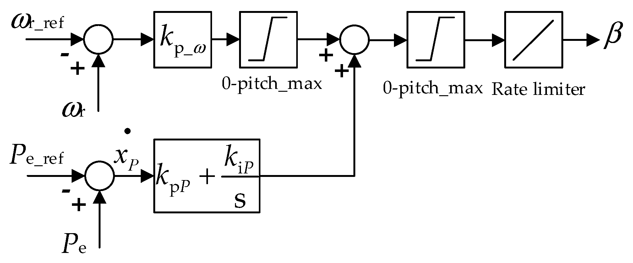
Adjustment of the pitch angle can change the energy capture capability of the wind turbine. When the generator speed exceeds the rated value, the pitch angle control is triggered to suppress the fluctuation caused by the adjustment of the speed controller. When the generator output exceeds the rated power, the pitch angle control is triggered to eliminate the imbalance between the input mechanical power and the rated electromagnetic power of the generator. The control block diagram of the pitch angle is shown in Figure 1.

2.2. Phase-Locked Loop (PLL) Model

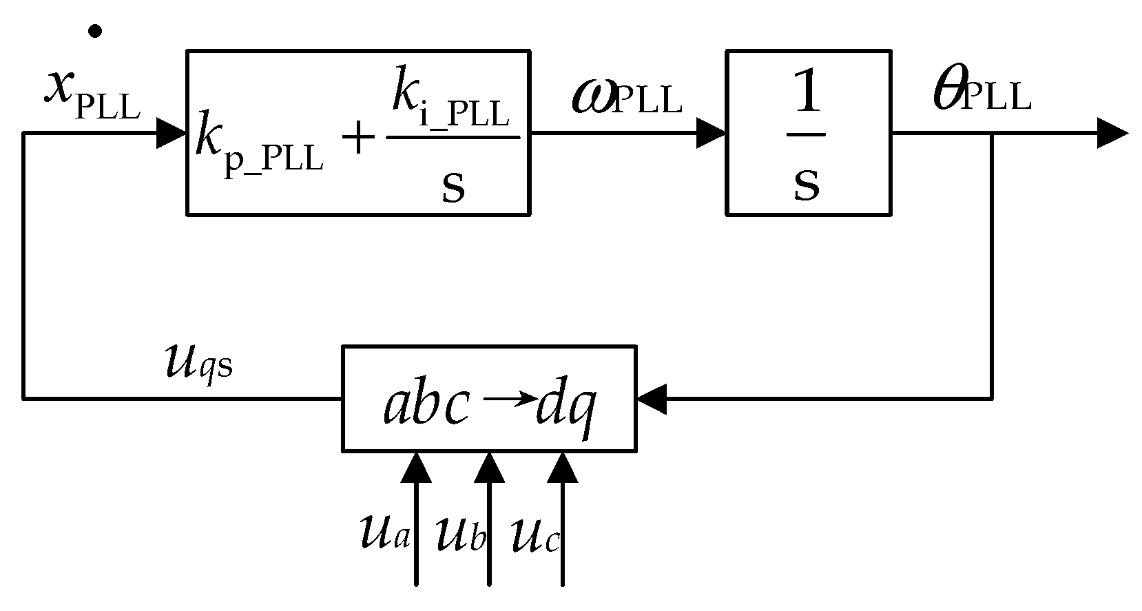
With respect to the stator voltage oriented vector control, the d-axis of the synchronous rotating reference frame coincides with the stator voltage. The accuracy of the oriented voltage phase is closely related to the control effect. Therefore, the PLL model shown in Figure 2 is applied in this paper. The dynamic equation can be expressed as follows:

$$\{\begin{array}{l}\frac{\mathrm{d}{x}_{\mathrm{PLL}}}{\mathrm{d}t}=u_{q\mathrm{s}}\\ \frac{\mathrm{d}{\theta }_{\mathrm{PLL}}}{\mathrm{d}t}={\omega }_{\mathrm{PLL}}-{\omega }_{\mathrm{b}}\\ {\omega }_{\mathrm{PLL}}=k_{\mathrm{i}\_\mathrm{PLL}}{x}_{\mathrm{PLL}}+k_{\mathrm{p}\_\mathrm{PLL}}{u}_{q\mathrm{s}}\end{array}$$

(1)

2.3. Shaft Model

The shaft model of a DFIG wind turbine system generally consists of wind turbine blades, a hub, a low-speed shaft, a gearbox, a high-speed shaft, and a generator rotor. This paper adopts the three-mass shaft model. The first mass stands for the wind turbine, including blades and a hub, while the second mass stands for the gearbox, and the third mass stands for the generator rotor. The springs of the low-speed shaft and high-speed shaft stand for their flexibility. The shaft model is described by the following equations:

$$\{\begin{array}{l}2H_{\mathrm{t}}\frac{\mathrm{d}{\omega }_{\mathrm{t}}}{\mathrm{d}t}=T_{\mathrm{M}}-D_{\mathrm{th}}({\omega }_{\mathrm{t}}-{\omega }_{\mathrm{h}})-K_{\mathrm{th}}{\theta }_{\mathrm{a}}-D_{\mathrm{t}}{\omega }_{\mathrm{t}}\\ 2H_{\mathrm{h}}\frac{\mathrm{d}{\omega }_{\mathrm{h}}}{\mathrm{d}t}=K_{\mathrm{th}}{\theta }_{\mathrm{a}}-K_{\mathrm{hr}}{\theta }_{\mathrm{b}}-D_{\mathrm{h}}{\omega }_{\mathrm{h}}+D_{\mathrm{th}}({\omega }_{\mathrm{t}}-{\omega }_{\mathrm{h}})-D_{\mathrm{hr}}({\omega }_{\mathrm{h}}-{\omega }_{\mathrm{r}})\\ 2H_{\mathrm{r}}\frac{\mathrm{d}{\omega }_{\mathrm{r}}}{\mathrm{d}t}=K_{\mathrm{hr}}{\theta }_{\mathrm{b}}+D_{\mathrm{hr}}({\omega }_{\mathrm{h}}-{\omega }_{\mathrm{r}})-D_{\mathrm{r}}{\omega }_{\mathrm{r}}-T_{\mathrm{e}}\\ \frac{\mathrm{d}{\theta }_{\mathrm{a}}}{\mathrm{d}t}={\omega }_{\mathrm{b}}({\omega }_{\mathrm{t}}-{\omega }_{\mathrm{h}})\\ \frac{\mathrm{d}{\theta }_{\mathrm{b}}}{\mathrm{d}t}={\omega }_{\mathrm{b}}({\omega }_{\mathrm{h}}-{\omega }_{\mathrm{r}})\end{array}$$

(2)

2.4. Generator Model

Assuming that the DFIG is an ideal motor that satisfies symmetry, sinusoidal, smoothness, and unsaturation, and the positive direction of the currents in stator and rotor windings is in accordance with the motor convention, the mathematical model is shown as Equations (3)–(5):

2.4.1. Voltage Equations of Stator and Rotor

$$\{\begin{array}{l}{u}_{\mathrm{s}}=R_{\mathrm{s}}{i}_{\mathrm{s}}+\mathrm{j}\frac{{\omega }_{\mathrm{PLL}}}{{\omega }_{\mathrm{b}}}{\psi }_{\mathrm{s}}+\frac{1}{{\omega }_{\mathrm{b}}}\frac{\mathrm{d}{\psi }_{\mathrm{s}}}{\mathrm{d}t}\\ u_{\mathrm{r}}=R_{\mathrm{r}}{i}_{\mathrm{r}}+\mathrm{j}\left(\frac{{\omega }_{\mathrm{PLL}}}{{\omega }_{\mathrm{b}}}-{\omega }_{\mathrm{r}}\right){\psi }_{\mathrm{r}}+\frac{1}{{\omega }_{\mathrm{b}}}\frac{\mathrm{d}{\psi }_{\mathrm{r}}}{\mathrm{d}t}\end{array}$$

(3)

2.4.2. Flux Linkage Equations

$$\{\begin{array}{l}{\psi }_{\mathrm{s}}=L_{\mathrm{ls}}{i}_{\mathrm{s}}+L_{\mathrm{m}}(i_{\mathrm{s}}+i_{\mathrm{r}})\\ {\psi }_{\mathrm{r}}=L_{\mathrm{lr}}{i}_{\mathrm{r}}+L_{\mathrm{m}}(i_{\mathrm{s}}+i_{\mathrm{r}})\end{array}$$

(4)

2.4.3. Electromagnetic Torque Equation

$$T_{\mathrm{e}}=L_{\mathrm{m}}(i_{q\mathrm{s}}{i}_{d\mathrm{r}}-i_{d\mathrm{s}}{i}_{q\mathrm{r}})$$

(5)

2.5. Grid-Side Filter

The grid-side filter adopts an inductor-capacitor low-pass filter. In order to facilitate modeling, it can be divided into two parts: the capacitance branch and the inductance branch.

2.5.1. Inductance Branch Equations

$$\{\begin{array}{l}{u}_{d\mathrm{s}}=R_{\mathrm{g}}{i}_{d\mathrm{g}}+\frac{L_{\mathrm{g}}}{{\omega }_{\mathrm{b}}}\frac{\mathrm{d}{i}_{d\mathrm{g}}}{\mathrm{d}t}-\frac{{\omega }_{\mathrm{PLL}}}{{\omega }_{\mathrm{b}}}{L}_{\mathrm{g}}{i}_{q\mathrm{g}}+u_{d\mathrm{g}}\\ u_{q\mathrm{s}}=R_{\mathrm{g}}{i}_{q\mathrm{g}}+\frac{L_{\mathrm{g}}}{{\omega }_{\mathrm{b}}}\frac{\mathrm{d}{i}_{q\mathrm{g}}}{\mathrm{d}t}+\frac{{\omega }_{\mathrm{PLL}}}{{\omega }_{\mathrm{b}}}{L}_{\mathrm{g}}{i}_{d\mathrm{g}}+u_{q\mathrm{g}}\end{array}$$

(6)

2.5.2. Capacitance Branch Equations

$$\{\begin{array}{l}\frac{C_{\mathrm{cr}}}{{\omega }_{\mathrm{b}}}\frac{\mathrm{d}{u}_{d\_\mathrm{cl}}}{\mathrm{d}t}=i_{d\mathrm{l}}-i_{d\mathrm{s}}-i_{d\mathrm{g}}+\frac{{\omega }_{\mathrm{PLL}}}{{\omega }_{\mathrm{b}}}{C}_{\mathrm{cr}}{u}_{q\_\mathrm{cl}}\\ \frac{C_{\mathrm{cr}}}{{\omega }_{\mathrm{b}}}\frac{\mathrm{d}{u}_{q\_\mathrm{cl}}}{\mathrm{d}t}=i_{q\mathrm{l}}-i_{q\mathrm{s}}-i_{q\mathrm{g}}-\frac{{\omega }_{\mathrm{PLL}}}{{\omega }_{\mathrm{b}}}{C}_{\mathrm{cr}}{u}_{d\_\mathrm{cl}}\\ u_{d\mathrm{s}}=R_{\mathrm{cr}}\left(i_{d\mathrm{l}}-i_{d\mathrm{s}}-i_{d\mathrm{g}}\right)+u_{d\_\mathrm{cl}}\\ u_{q\mathrm{s}}=R_{\mathrm{cr}}\left(i_{q\mathrm{l}}-i_{q\mathrm{s}}-i_{q\mathrm{g}}\right)+u_{q\_\mathrm{cl}}\end{array}$$

(7)

2.6. Converter Model

2.6.1. DC Capacitor Model

Dual pulse width modulation (PWM) converters can be classified into a rotor-side converter and a grid-side converter. When the active power of the two converters are unequal, the unbalanced power will cause the DC capacitor voltage to fluctuate. The mathematical model can be expressed as:

$$C_{\mathrm{dc}}{U}_{\mathrm{dc}}\frac{\mathrm{d}{U}_{\mathrm{dc}}}{\mathrm{d}t}=\frac{3}{2}(u_{d\mathrm{g}}{i}_{d\mathrm{g}}+u_{q\mathrm{g}}{i}_{q\mathrm{g}}-u_{d\mathrm{r}}{i}_{d\mathrm{r}}-u_{q\mathrm{r}}{i}_{q\mathrm{r}})$$

(8)

2.6.2. Control System of Rotor-Side Converter

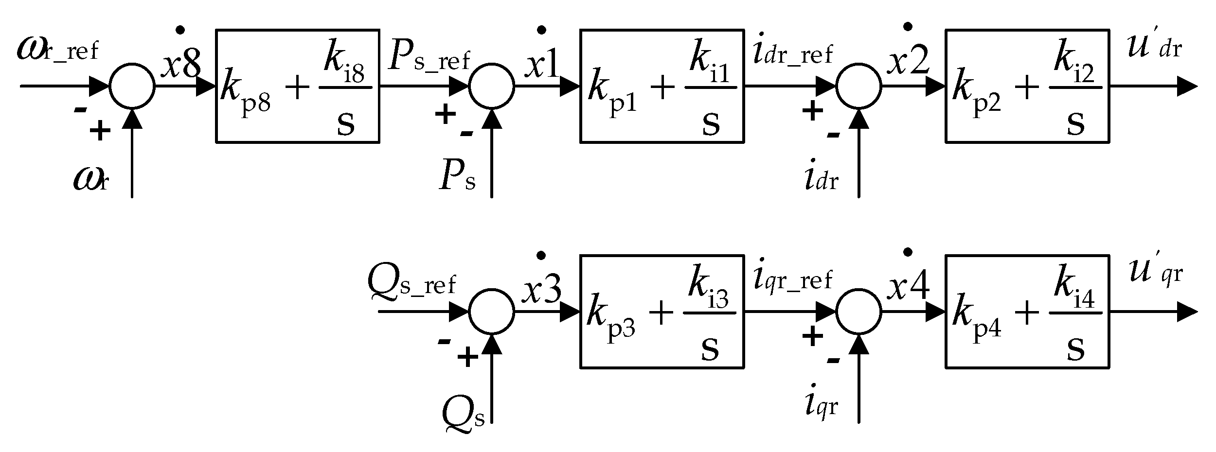
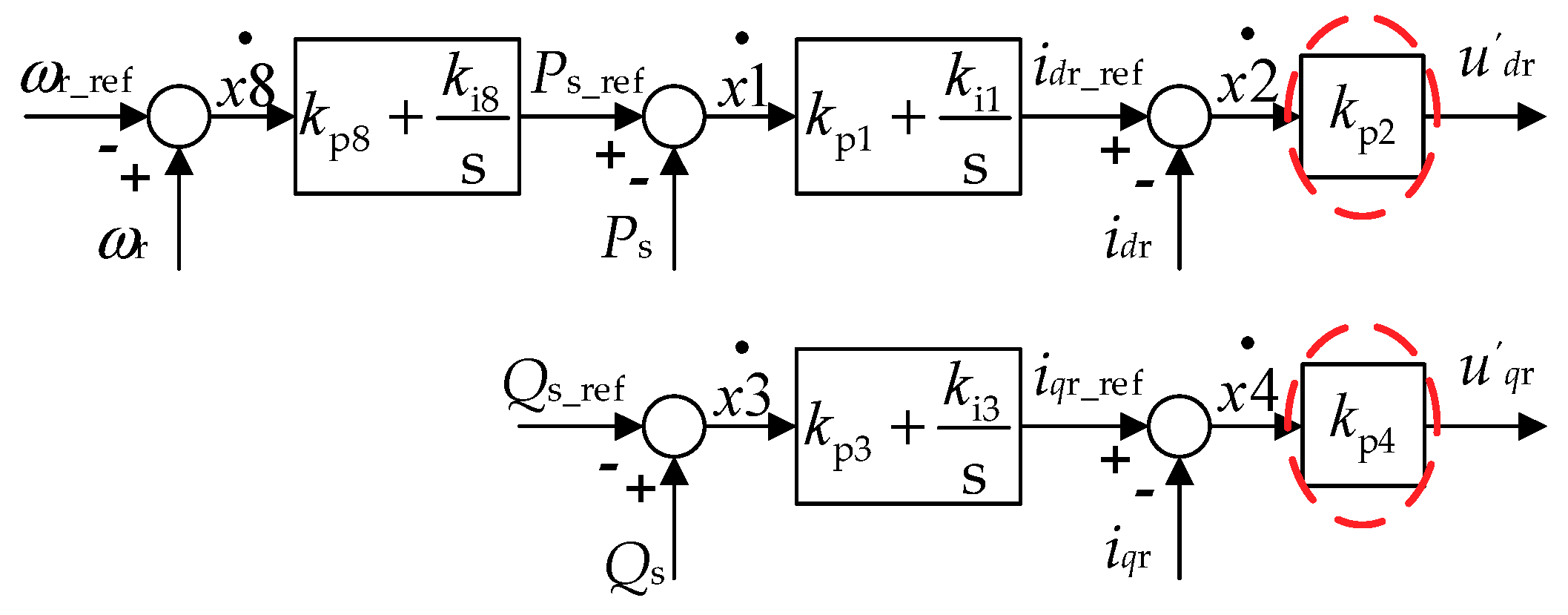
There are two main objectives for the control of the rotor-side converter. The first is to achieve maximum wind energy tracking under the premise of variable speed and constant frequency, the key of which lies in the control of generator speed or active power. The second is to control the reactive power output by the DFIG to ensure the operation stability of the power grid. The control block diagram is shown in Figure 3.

Therefore, the output voltage of the rotor-side converter can be expressed as:

$$\{\begin{array}{l}{u}_{d\mathrm{r}}=u_{d\mathrm{r}}^{\prime }-(\frac{{\omega }_{\mathrm{PLL}}}{{\omega }_{\mathrm{b}}}-{\omega }_{\mathrm{r}})\sigma L_{\mathrm{r}}{i}_{q\mathrm{r}}+R_{\mathrm{r}}{i}_{d\mathrm{r}}+{\omega }_{\mathrm{r}}\frac{L_{\mathrm{m}}}{L_{\mathrm{s}}}{\psi }_{q\mathrm{s}}+\frac{L_{\mathrm{m}}}{L_{\mathrm{s}}}(u_{d\mathrm{s}}-R_s{i}_{d\mathrm{s}})\\ u_{q\mathrm{r}}=u_{q\mathrm{r}}^{\prime }+(\frac{{\omega }_{\mathrm{PLL}}}{{\omega }_{\mathrm{b}}}-{\omega }_{\mathrm{r}})\sigma L_{\mathrm{r}}{i}_{d\mathrm{r}}+R_{\mathrm{r}}{i}_{q\mathrm{r}}-{\omega }_{\mathrm{r}}\frac{L_{\mathrm{m}}}{L_{\mathrm{s}}}{\psi }_{d\mathrm{s}}+\frac{L_{\mathrm{m}}}{L_{\mathrm{s}}}(u_{q\mathrm{s}}-R_{\mathrm{s}}{i}_{q\mathrm{s}})\\ \sigma =1-\frac{L_{\mathrm{m}}^2}{L_{\mathrm{s}}{L}_{\mathrm{r}}}\end{array}$$

(9)

2.6.3. Control System of Grid-Side Converter

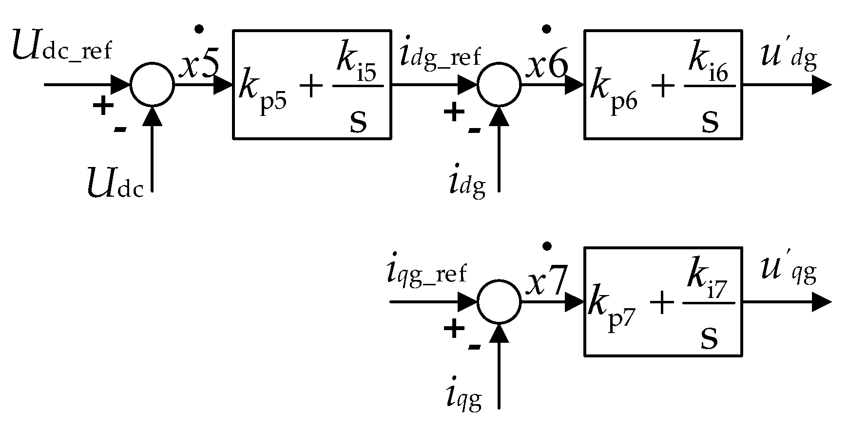
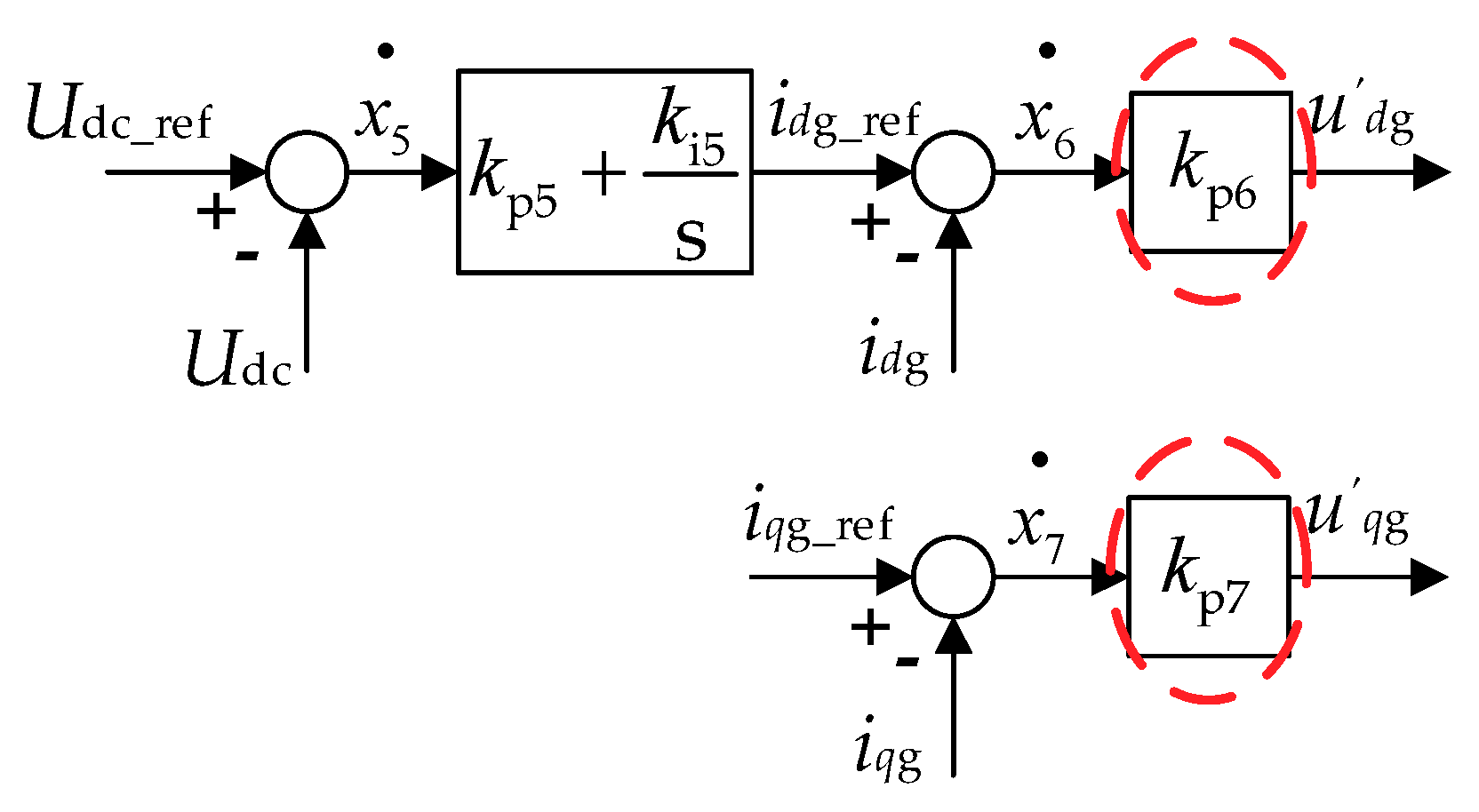
The main function of the grid-side converter is to maintain the stability of the DC bus voltage and achieve the control of alternating current side power factor. The control block diagram is shown in Figure 4.

Therefore, the output voltage of the grid-side converter can be expressed as:

$$\{\begin{array}{l}{u}_{d\mathrm{s}}=R_{\mathrm{g}}{i}_{d\mathrm{g}}+u_{d\mathrm{g}}^{\prime }-{\omega }_{\mathrm{s}}{L}_{\mathrm{g}}{i}_{q\mathrm{g}}+u_{d\mathrm{g}}\\ u_{q\mathrm{s}}=R_{\mathrm{g}}{i}_{q\mathrm{g}}+u_{q\mathrm{g}}^{\prime }+{\omega }_{\mathrm{s}}{L}_{\mathrm{g}}{i}_{d\mathrm{g}}+u_{q\mathrm{g}}\end{array}$$

(10)

2.7. Transmission Line

Considering that the excitation impedance of the transformer is large, the transmission line and the transformer are equivalent to the Resistor-inductor model by ignoring the excitation branch of the transformer. The dynamic equations is shown as Equation (11):

$$\{\begin{array}{l}\frac{L_{\mathrm{l}}}{{\omega }_{\mathrm{b}}}\frac{\mathrm{d}{i}_{d\mathrm{l}}}{\mathrm{d}t}=u_{d\_\mathrm{pcc}}-u_{d\mathrm{s}}-R_{\mathrm{l}}{i}_{d\mathrm{l}}+\frac{{\omega }_{\mathrm{PLL}}}{{\omega }_{\mathrm{b}}}{L}_{\mathrm{l}}{i}_{q\mathrm{l}}\\ \frac{L_{\mathrm{l}}}{{\omega }_{\mathrm{b}}}\frac{\mathrm{d}{i}_{q\mathrm{l}}}{\mathrm{d}t}=u_{q\_\mathrm{pcc}}-u_{q\mathrm{s}}-R_{\mathrm{l}}{i}_{q\mathrm{l}}-\frac{{\omega }_{\mathrm{PLL}}}{{\omega }_{\mathrm{b}}}{L}_{\mathrm{l}}{i}_{d\mathrm{l}}\end{array}$$

(11)

3. Electromagnetic Transient Modeling and Electromechanical Transient Modeling of the DFIG Wind Turbine System

3.1. General Principle of Model Reduction

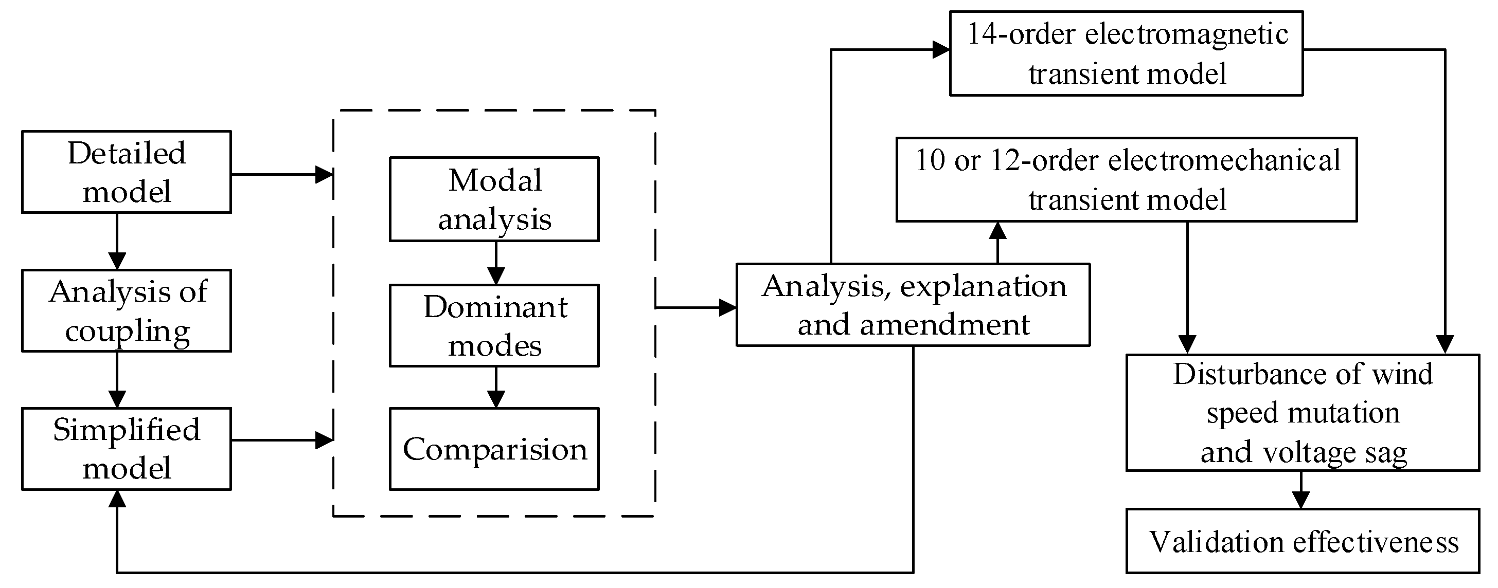
This section focuses on the detailed process of model reduction. The general principle is as follows. Firstly, the small disturbance model of the DFIG wind turbine system with the equilibrium point at the maximum power tracking (MPPT) stage is constructed for exploring the multi-time scale characteristics of the DFIG wind turbine system. Then, we take the variation in eigenvalues of the DFIG wind turbine system before and after the order reduction as the initial rationality criterion for model reduction, which is aligned with the analysis of the coupling between variables and the system, as well as the coupling between variables of different time scales. Thus, the primary simplified model and different reduced-order models are obtained. Finally, the validity of the proposed simplified electromagnetic model and electromechanical model is validated under simulation of large disturbance situations. A brief outline of the model reduction process is shown in Figure 5.

3.2. Multi-Time Scale Characteristics Analysis of the DFIG Wind Turbine System Based on the Detailed Model

Most of the time, wind turbines work at the maximum power point tracking (MPPT) stage when the pitch angle is a fixed value. The DFIG wind turbine system analyzed in this paper works at this stage, so the pitch angle control system is not included in the following analysis.

Equation (12) can be applied to express the detailed mathematical model of the DFIG wind turbine system in Section 1. Using first-order Taylor expansion at the equilibrium point of the system, the linearized system is obtained as shown in Equation (13):

$$\{\begin{array}{l}\frac{\mathrm{d}\mathit{x}}{\mathrm{d}t}=f\left(\mathit{x},\mathit{y},\mathit{z}\right)\\ \mathit{y}=g\left(\mathit{x},\mathit{y},\mathit{z}\right)\end{array}$$

(12)

$$\{\begin{array}{l}\frac{\mathrm{d}\Delta \mathit{x}}{\mathrm{d}t}=\mathit{A}\Delta \mathit{x}+\mathit{B}\Delta \mathit{y}+\mathit{C}\Delta \mathit{z}\\ 0=\mathit{D}\Delta \mathit{x}+\mathit{E}\Delta \mathit{y}+\mathit{F}\Delta \mathit{z}\end{array}$$

(13)

where x is the state variable vector of the DFIG wind turbine system; y is the output variable vector; and z is the input variable vector.

Then, we transform Equation (13) into Equation (14):

$$\{\begin{array}{l}\frac{\mathrm{d}\Delta \mathit{x}}{\mathrm{d}t}=\mathit{H}\Delta \mathit{x}+\mathit{K}\Delta \mathit{z}\\ \mathit{H}=\mathit{A}-\mathit{B}{\mathit{F}}^{-1}\mathit{E}\\ \mathit{K}=\mathit{C}-\mathit{B}{\mathit{F}}^{-1}\mathit{G}\end{array}$$

(14)

where H stands for the state matrix.

Then, the change trend of each state variable under small disturbance can be derived as shown in Equation (15):

$$\Delta \mathit{x}={\displaystyle {\int }_0^t{e}^{\mathit{H}(t-\tau )}}\mathit{K}\Delta \mathit{z}(\tau )d\tau +e^{\mathit{H}t}\Delta {\mathit{x}}_0$$

(15)

Calculating the eigenvalues of the state matrix H and the participation factors of the linearized system, the correlation degrees between each state variable and each mode are obtained, and the state variables strongly related to each mode are selected. The details are shown in

Table 1. Dominant modes of state variables for a doubly-fed induction generator (DFIG) wind turbine system.

Symbol	Eigenvalue	State Parameter
λ1	−7.0633 × 103	Δψdr
λ2	8.0866 × 102 ± 4.5519 × 103i	Δidl, Δiql, Δud_cl, Δuq_cl
λ3	6.8350 × 102 ± 4.0238 × 103i	Δidl, Δiql, Δud_cl, Δuq_cl, Δψqr, Δψqs
λ4	−1.3758 × 103	Δψqr, Δψqs
λ5	4.6819 × 102 ± 7.3983 × 102i	ΔUdc, Δidg, Δψdr, Δidl, Δψds
λ6	−2.6670 ± 3.1314 × 102i	Δψds, Δψqs
λ7	−863.1075	Δiqg
λ8	−159.8480	ΔθPLL, ΔxPLL
λ9	−92.8698	Δx3
λ10	−52.9091	Δx5
λ11	−48.0355	Δx1
λ12	−19.9381	ΔxPLL, ΔθPLL
λ13	−2.2099 ± 45.6153i	Δωh, Δθb
λ14	−13.3094	Δx4
λ15	−6.0241	Δx6
λ16	−0.8089 ± 6.4119i	Δωr, Δθa
λ17	−0.1657 ± 0.1737i	Δωt, Δx8
λ18	−1.6000	Δx2
λ19	−6.0664	Δx7

.

In this paper, the decay speed and the change speed of each mode are represented by time constant T = −1/Re and natural frequency f = (Re² + Im²)^1/2 (where Re and Im are the real part and the imaginary part of the eigenvalue, respectively). From Table 1, it can be seen that the time scale of the DFIG wind turbine system is distributed in the range of milliseconds to minutes, and there are obvious multi-time scale characteristics. Among them, the time scale of mechanical variables such as ω and θ is much smaller than that of electrical variables such as ψ and i, so the decay speed of the mechanical part is much slower.

3.3. Model Reduction and Rationality Analysis

3.3.1. 21-Order Preliminary Simplified Model and Its Rationality Analysis

The transient process of a DFIG wind turbine system can be divided into an electromagnetic transient process and an electromechanical transient process according to the time scale. Electromagnetic transient simulation mainly studies the dynamic process of electromagnetic phenomena of voltage and current within one fundamental frequency cycle time (50 Hz, 20 ms). The time scale of an electromechanical transient process is generally 0.1–10 s.

Firstly, in the electromagnetic transient process time scale, the integral link of the PI controller in the converter control system has not enough time to store much energy. Thus, it can be considered that the dynamics of control system is determined by the proportion link of the PI controller. While in the electromechanical transient process time scale, under the condition that no disturbance occurs in the internal variables of the inner loop of the control system, it can be considered that the inner loop controller of the control system can completely track the output of the outer loop of the control system, i.e., the input amplitude of the inner loop controller is so small that the accumulation of the integral link of the inner loop controller is neglectable. Therefore, the integral link of the inner loop controllers in Figure 3 and Figure 4 can be neglected, and the simplified control systems of the dual PWM converters are shown in Figure 6 and Figure 7.

Then, according to Equation (10), the additional items of the grid-side control system account for the dynamics of the stator voltage. The change of the stator voltage does not affect the voltage across the filter. The current of the filter is determined by the grid-side converter control system, and the q-axis current of the grid-side filter is neglectable. Therefore, a 21-order DFIG wind turbine system model can be established. In order to verify the impact of the ignored variables on the overall trend of the system dynamics, the eigenvalues of the 21-order simplified model are calculated. The results are shown in

Table 2. Dominant modes of state variables for a 21-order simplified model.

Symbol	Eigenvalue	State Parameter
λ1	−7.0650 × 103	Δψdr
λ2	8.0835 × 102 ± 4.5519 × 103i	Δidl, Δiql, Δud_cl, Δuq_cl
λ3	6.8330 × 102 ± 4.0242 × 103i	Δidl, Δiql, Δud_cl, Δuq_cl, Δψqr, Δψqs
λ4	−1.3911 × 103	Δψqr, Δψqs
λ5	4.7127 × 102 ± 7.3765 × 102i	ΔUdc, Δidg, Δψdr, Δidl, Δψds
λ6	−2.6772 ± 3.1315 × 102i	Δψds, Δψqs
λ8	−159.8567	ΔθPLL, ΔxPLL
λ9	−91.6510	Δx3
λ10	−52.9364	Δx5
λ11	−48.0253	Δx1
λ12	−19.9380	ΔxPLL, ΔθPLL
λ13	−2.2099 ± 45.6153i	Δωh, Δθb
λ16	−0.8089 ± 6.4119i	Δωr, Δθa
λ17	−0.1657 ± 0.1737i	Δωt, Δx8

.

Comparing Table 1 and Table 2, it can be concluded that in the case of neglecting the integral link of the inner loop controller of the control system, as well as the q-axis current dynamics of the grid-side filter, the eigenvalues of other modes in the system are little affected. Thus, the obtained 21-order simplified model is reasonable. Furthermore, the reduced-order model of a DFIG wind turbine system is respectively presented according to the time scales of the electromagnetic transient process and the electromechanical transient process, based on the 21-order simplified model.

3.3.2. Electromagnetic Transient Process Modeling

1. Analysis of the 15-order electromagnetic transient model

In the electromagnetic transient time scale, the work done by the imbalance of shaft torque to the generator rotor is little, while the inertia of the generator rotor is large. According to Equation (2), the generator speed is hardly changed. Therefore, the influence of the shaft on the DFIG wind turbine system can be ignored. I.e., assuming that the state variables of the shaft (ω_t, ω_h, ω_r, θ_a, θ_b, and x8) are constants, the model can be further simplified to 15 orders. In this case, the eigenvalues of the reduced-order model are shown in

Table 3. Dominant modes of state variables for a 15-order simplified model.

Symbol	Eigenvalue	State Parameter
λ1	−7.0658 × 103	Δψdr
λ2	8.0833 × 102 ± 4.5519 × 103i	Δidl, Δiql, Δud_cl, Δuq_cl
λ3	6.8328 × 102 ± 4.0242 × 103i	Δidl, Δiql, Δud_cl, Δuq_cl, Δψqr, Δψqs
λ4	−1.3911 × 103	Δψqr, Δψqs
λ5	4.7125 × 102 ± 7.3766 × 102i	ΔUdc, Δidg, Δψdr, Δidl, Δψds
λ6	−2.6826 ± 3.1315 × 102i	Δψds, Δψqs
λ8	−159.8707	ΔθPLL, ΔxPLL
λ9	−91.6502	Δx3
λ10	−52.9476	Δx5
λ11	−49.2921	Δx1
λ12	−19.9424	ΔxPLL, ΔθPLL

.

Comparing Table 2 and Table 3, it can be seen that the ignorance of the dynamic process of the state variables of the shaft module has little impact on the other modes of the system, and can well represent the electromagnetic transient process of the system.

2. Analysis of the 14-order electromagnetic transient model

Further simplification can be applied by neglecting the variables that have little effect on the overall trend of the DFIG wind turbine system. For example, the ratio of the integral link gain to the proportional link gain of the PI controller of the PLL is small; the accumulation of the integral link is neglectable compared to the output of the proportional link in a short time. Therefore, the integral link of the controller of the PLL can be ignored, and the model can be further simplified to 14 orders. In this case, the eigenvalues of the reduced-order model are shown in

Table 4. Dominant modes of state variables for a 14-order simplified model.

Symbol	Eigenvalue	State Parameter
λ1	−7.0658 × 103	Δψdr
λ2	8.0829 × 102 ± 4.5519 × 103i	Δidl, Δiql, Δud_cl, Δuq_cl
λ3	6.8314 × 102 ± 4.0242 × 103i	Δidl, Δiql, Δud_cl, Δuq_cl, Δψqr, Δψqs
λ4	−1.3913 × 103	Δψqr, Δψqs
λ5	4.7126× 102 ± 7.3767 × 102i	ΔUdc, Δidg, Δψdr, Δidl, Δψds
λ6	−2.6839 ± 3.1315 × 102i	Δψds, Δψqs
λ8	−180.0049	ΔθPLL
λ9	−91.8212	Δx3
λ10	−52.9166	Δx5
λ11	−49.0349	Δx1

.

Comparing Table 2 and Table 4, it can be seen that only the characteristic values corresponding to the PLL have changed greatly because of the ignorance of the integral link. Since the relative phase angle θ_PLL is output through the integral link, it may not affect the dynamics of the DFIG wind turbine system in a short time. Therefore, it is reasonable to ignore the integral link of the PLL controller.

3. Analysis of Other Reduced-Order Electromagnetic Transient Model of the DFIG Wind Turbine System

In the case of lower precision requirements, further simplification can be adopted on the basis of the abovementioned 14-order simplified model. Firstly, the integral link of the outer ring controller of the control system can be ignored, but this reduction is only effective in the smaller time scale (less than 10 ms). The reason is that since the ratio of the integral link gain to the proportional link gain in the outer ring controller is relatively large, i.e., the cumulative amount of the integral link has a great influence on the output of the proportional link, the time scale at which the simplified model fit the output curve of the detailed model will be reduced. Moreover, without the integral link, the control system cannot make an adjustment without a difference. In a larger time scale (from 10 ms to minutes), the simplified model cannot follow the output curve of the detailed model. In other words, ignoring the integral link of the PI controller of the outer loop of the control system is only suitable for studying the variation trend of each variable in an electromagnetic transient process time scale.

Secondly, if only the dynamic process of generator-side variables need analysis, the dynamic process of the grid-side filter and the DC voltage can be ignored. The reason is that according to the structure of the DFIG wind turbine system, the generator-side variables are not directly affected by the DC voltage and the grid-side filter. The output of the PLL can be assumed constant for further simplification if the dynamic process of the PLL is ignored. The validity analysis of the model simplifications is not repeated here.

3.3.3. Electromechanical Transient Process Modeling

1. Analysis of the six-order electromechanical transient model

According to Table 1, the electrical variables and the control variables change faster than the mechanical variables. Ideally, the electrical variables and control variables mutate instantly in the electromechanical transient process. Thus, the simplified six-order electromechanical transient model is obtained; its eigenvalues are shown in

Table 5. Dominant modes of state variables for the six-order simplified model.

Symbol	Eigenvalue	State Parameter
λ13	−2.2384 ± 45.5741i	Δωh, Δθb
λ16	−0.7968 ± 6.3449i	Δωr, Δθa
λ17	−0.1654 ± 0.1733i	Δωt, Δx8

.

Comparing Table 2 and Table 5, it can be seen that the eigenvalues of the DFIG wind turbine system change greatly after ignoring the dynamic process of the electrical variables and control variables. This shows the dynamic process of the ignored variables has a great influence on the generator speed, and the six-order simplified model may cause a big error in simulation.

2. Analysis of the eight-order electromechanical transient model

According to Equation (4), the change of the stator flux linkage of the generator will cause the change of the rotor current in the electromechanical time scale. However, this is due to the effect of the rotor current inner loop in the rotor converter control system, as well as the response speed of the rotor flux linkage being far greater than that of the stator flux linkage (see Table 1). The rotor flux linkage will quickly follow the change trend of the stator flux linkage, and the stator and rotor currents are almost changeless, i.e., the electromagnetic torque hardly changes. Therefore, it can be considered that the stator flux linkage does not affect the generator speed.

Moreover, the grid-side converter control system, which helps maintain the stability of the DC capacitance, is uncoupled with the rotor-side converter, and will not affect the stator and rotor currents. Therefore, the stator flux linkage, the grid-side state variables, and the inner loop controller of the control system have little influence on the generator electromagnetic torque. According to the natural frequency distribution in Table 1, the intermediate variables of the outer loop (x1, x3) of the control system are added to the slow variables to better fit the dynamic curve of the shaft module, and then the eight-order electromechanical transient process model is obtained. The eigenvalues are shown in

Table 6. Dominant modes of state variables for an eight-order simplified model.

Symbol	Eigenvalue	State Parameter
λ9	−85.7512	Δx3
λ11	−47.3103	Δx1
λ13	−2.2097 ± 45.6144i	Δωh, Δθb
λ16	−0.8087 ± 6.4113i	Δωr, Δθa
λ17	−0.1657 ± 0.1737i	Δωt, Δx8

.

Comparing Table 2 and Table 6, it can be seen that when the intermediate variables of the outer loop of the control system are taken into account, the error of the shaft dominant mode eigenvalues is reduced, and the overall dynamics of the shaft module will be better modulated. Meanwhile, the dominant mode eigenvalues of the outer loop intermediate variables change significantly. This is due to the ignorance of the dynamic process of the state variables corresponding to the outer loop control variables, and what corresponds to the power outer loop is the rotor flux linkage.

3. Analysis of the 10-order electromechanical transient model

The rotor flux linkage changes rapidly in the transient dynamics according to Table 1, and thus can be ignored to accelerate the simulation speed. However, this may result in the collapse of the whole system. This is because when the dynamics of the rotor flux linkage is ignored, the rotor flux linkage will mutate if a large disturbance is introduced to the model, the accuracy of the control system will be reduced, and the errors will be magnified. Therefore, it is suggested that the rotor flux linkage dynamics should be considered in the electromechanical time scale, and thus, the 10-order electromechanical model is achieved. The eigenvalues are shown in

Table 7. Dominant modes of state variables for the 10-order simplified model.

Symbol	Eigenvalue	State Parameter
λ1	−7.3856 × 103	Δψdr
λ4	−1.0612 × 103	Δψqr
λ9	−93.2471	Δx3
λ11	−47.6236	Δx1
λ13	−2.2099 ± 45.6147i	Δωh, Δθb
λ16	−0.8088 ± 6.4113i	Δωr, Δθa
λ17	−0.1657 ± 0.1737i	Δωt, Δx8

.

Comparing Table 2, Table 6, and Table 7, it can be seen that after adding the rotor flux linkage dynamics, the errors of the eigenvalues of the outer loop of the control system and the shaft dominant mode are greatly improved, but it has a great influence on the eigenvalues corresponding to the rotor flux linkage dominant mode. Since the time constant of the rotor flux linkage is small and the dynamics of the rotor flux linkage decay fast, the influence of the rotor flux linkage on the shaft can be neglected. Therefore, the error of the eigenvalues corresponding to the rotor flux linkage dominant mode can be neglected.

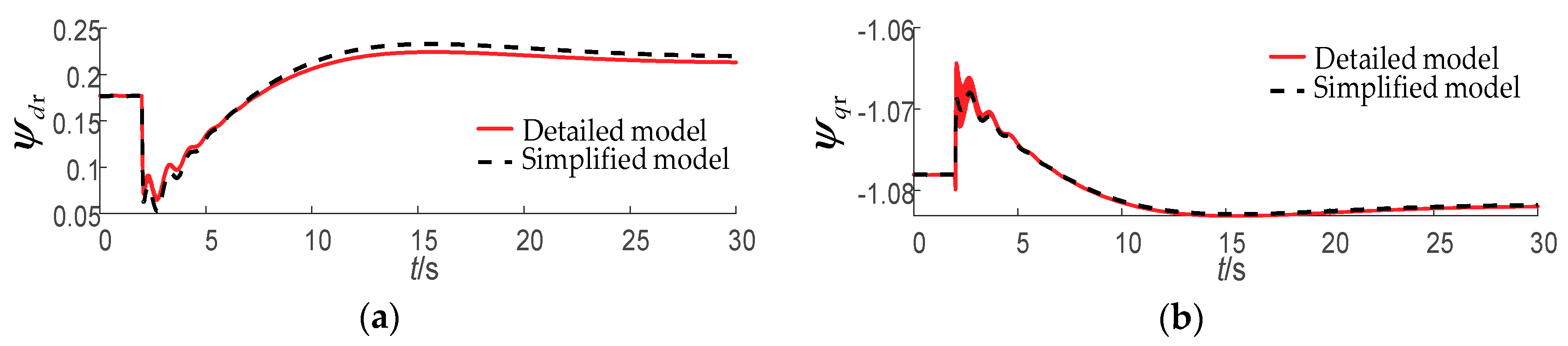
Since the dynamic process of the stator-side energy storage element is neglected and the change trend of the stator-side state variables are determined by the rotor flux linkage, the error of the rotor flux linkage is adopted to estimate the coincidence of the output characteristics of the 10-order simplified model and the detailed model. The dynamics of the rotor flux linkage for the detailed model and 10-order simplified model when the wind speed changes from 10 m/s to 11 m/s are shown as Figure 8. From Figure 8, it can be seen that the rotor flux balance point of the simplified system has been offset, which illustrates the analysis on Table 7.

4. Analysis of the 12-order electromechanical transient model

The offset of the balance point of the 10-order simplified model is caused by the ignorance of the PLL in the electromechanical time scale. The dynamics of the PLL is directly related to the rotation speed of the rotating reference coordinate system. Ignoring the dynamics of the PLL will cause the missing of the deviation of the d-axis and q-axis voltage components at the point of common coupling (PCC) points, which makes the system balance point deviate. Therefore, taking into account the dynamics of the PLL in the electromechanical time scale, a 12-order electromechanical transient model is established, and the eigenvalues of the reduced-order model are shown in

Table 8. Dominant modes of state variables for the 12-order simplified model.

Symbol	Eigenvalue	State Parameter
λ1	−3.6741 × 103	Δψdr
λ4	−1.1036 × 103	Δψqr
λ8	−160.4084	ΔθPLL, ΔxPLL
λ9	−93.4418	Δx3
λ11	−48.1219	Δx1
λ12	−19.9347	ΔxPLL, ΔθPLL
λ13	−2.2099 ± 45.6154i	Δωh, Δθb
λ16	−0.8089 ± 6.4119i	Δωr, Δθa
λ17	−0.1657 ± 0.1737i	Δωt, Δx8

.

Comparing Table 2 and Table 8, the time constant of the d-axis flux linkage of the rotor doubles after taking into account the dynamics of the PLL in the electromechanical time scale. Meanwhile, the response speed of the d-axis flux linkage of the rotor is still far greater than that of other state variables of the simplified model. Therefore, the influence caused by the change of the time constant of the d-axis flux linkage of the rotor can be ignored.

5. Notification of the 12-order model and 10-order model

It should be noted that although the 12-order electromechanical transient model has higher precision than the 10-order model, its stability performance is worse under voltage sag conditions. The reason is that for the 12-order model, a large angular frequency error from the phase-lock loop output may occur because of the consideration of the dynamics of the phase-lock loop and the ignorance of the energy storage components in the stator side of the DFIG wind turbine system, resulting in the crash of the entire system.

Therefore, under voltage sag conditions, the 10-order electromechanical transient model should be adopted instead of the 12-order model. Under other conditions except voltage sag, the 12-order electromechanical transient model can be selected to improve the simulation accuracy.

3.4. Choice of the Simulation Models

In this paper, considering the simulation speed and simulation accuracy of the model, the models represented by Table 4 and Table 7 or Table 8 are selected as the electromagnetic transient simulation model and the electromechanical transient simulation model. Compared with the 26-order detailed model, the order of the simplified models are greatly reduced. In which, the electromagnetic transient simulation model of Table 4 is a 14-order model, and the electromechanical transient simulation model of Table 7 or Table 8 is a 10 or 12-order model (depending on the working conditions).

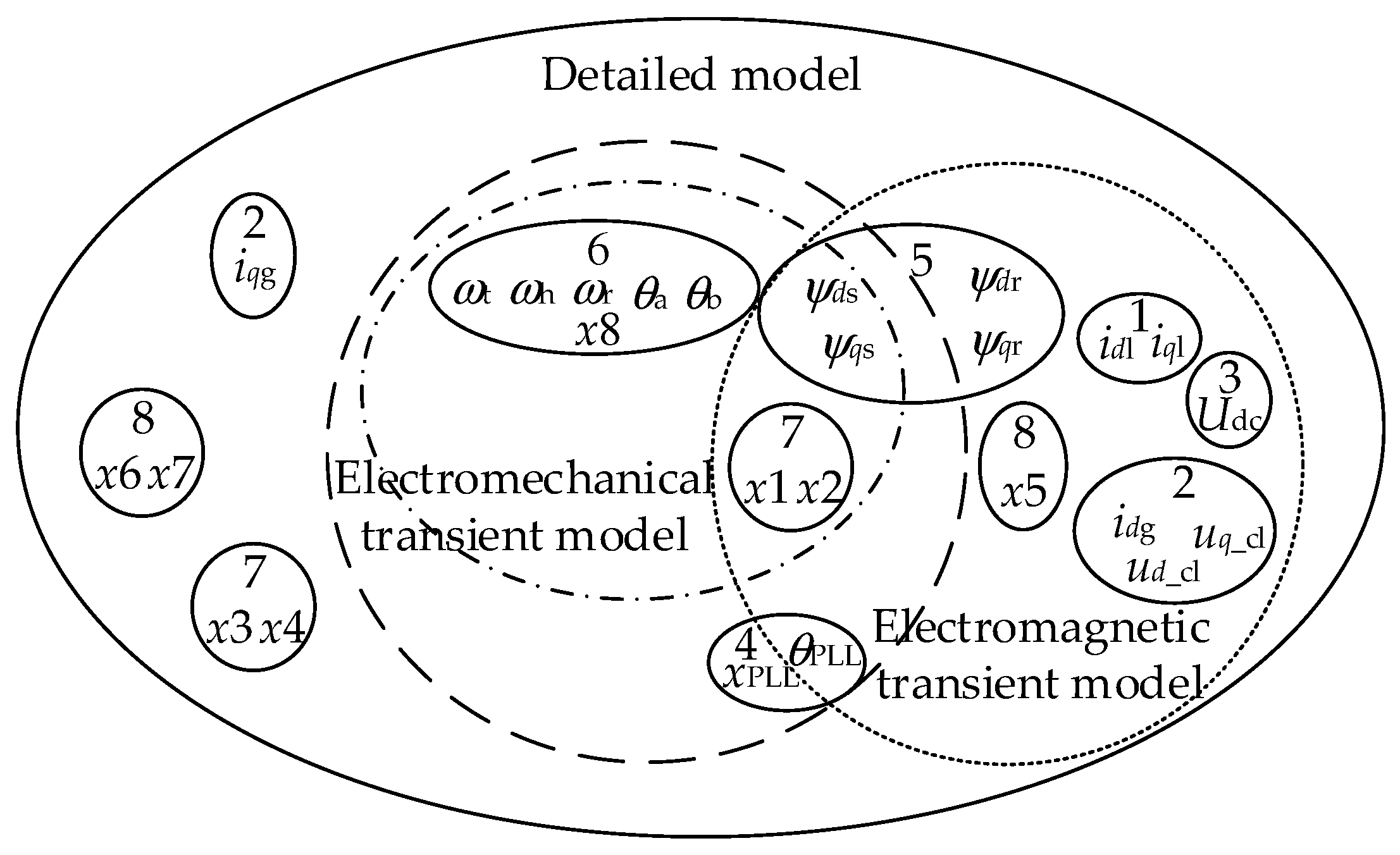
The distribution of the state variables of the detailed model and the 14-order and 12-order simplified models is shown in Figure 9. The symbols 1 to 8 are explained as follows:

• 1-State variables of the interface line module.
• 2-State variables of the grid-side filter module.
• 3-State variables of the DC capacitor module.
• 4-State variables of the PLL module.
• 5-State variables of the induction generator module.
• 6-State variables of the shaft module.
• 7-State variables of the rotor-side control system.
• 8-State variables of the grid-side control system.

What’s more, in real applications, other simplified models represented by Table 3, Table 5 and Table 6 could be adopted according to different research goals and the requirements of accuracy and simulation speed.

4. Simulations

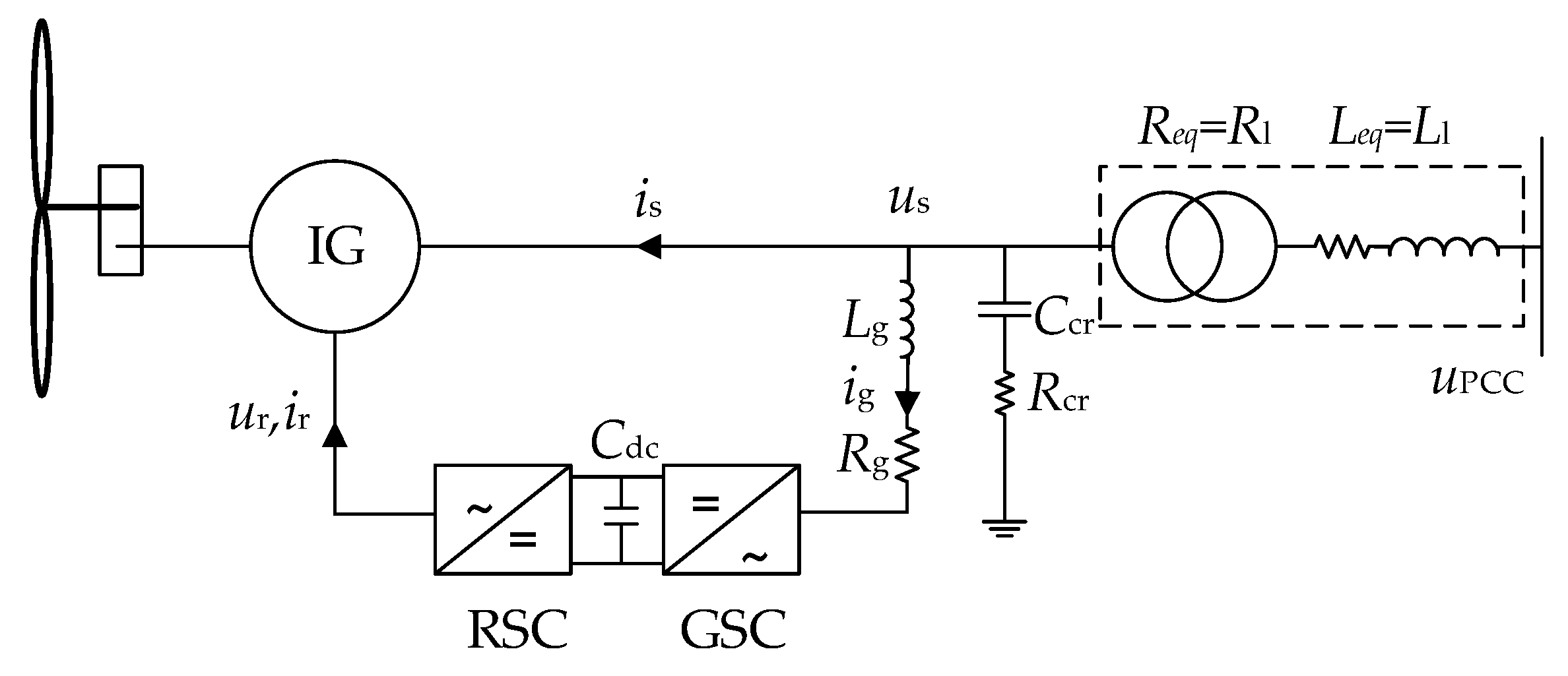
Appendix A gives the parameters of the 1.5-MW, 690-V DFIG that was used for the study. The power network of a DFIG wind turbine connected to the infinite bus, as shown in Figure 10, is applied to investigate the performance of the reduced-order models of the DFIG wind turbine system. The simulation consists of large disturbance conditions of wind speed mutation and voltage sag. The rationality of the simplified models is verified by the comparison of dynamic characteristics between the detailed model and simplified models.

4.1. Simulations under Wind Speed Mutation

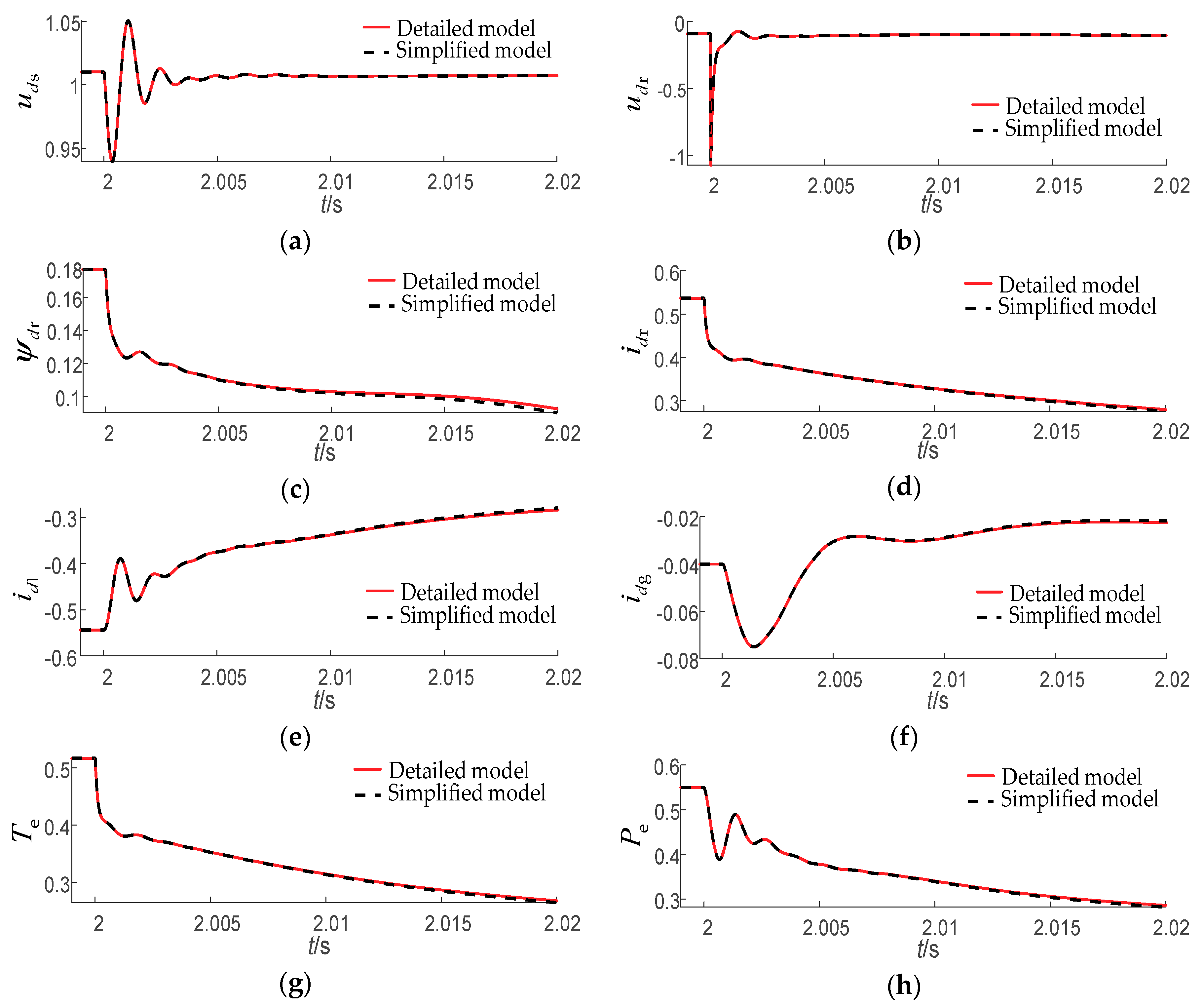
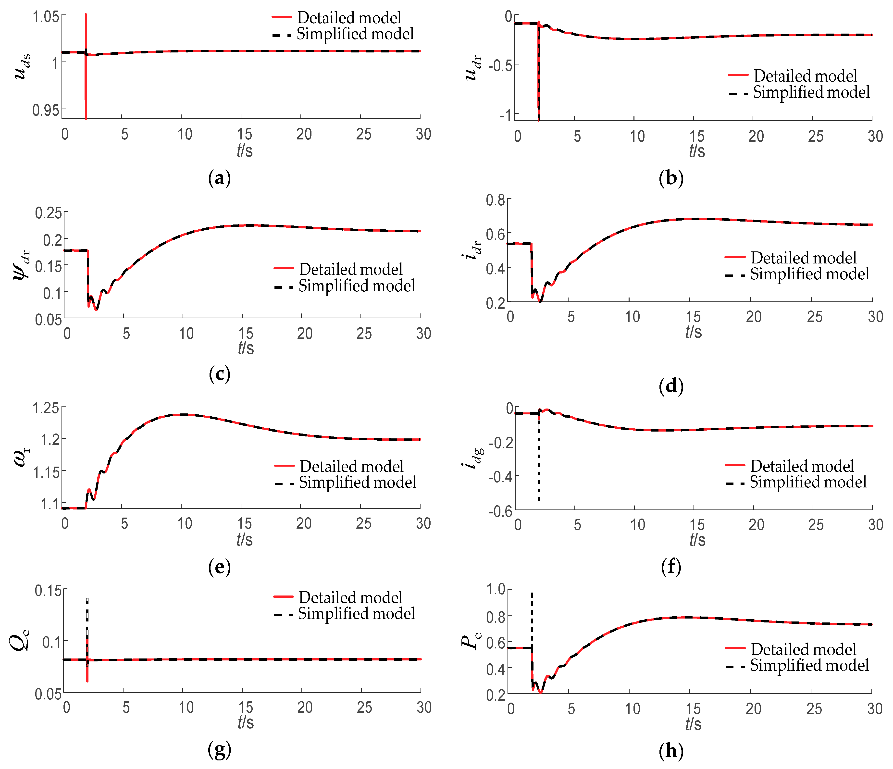
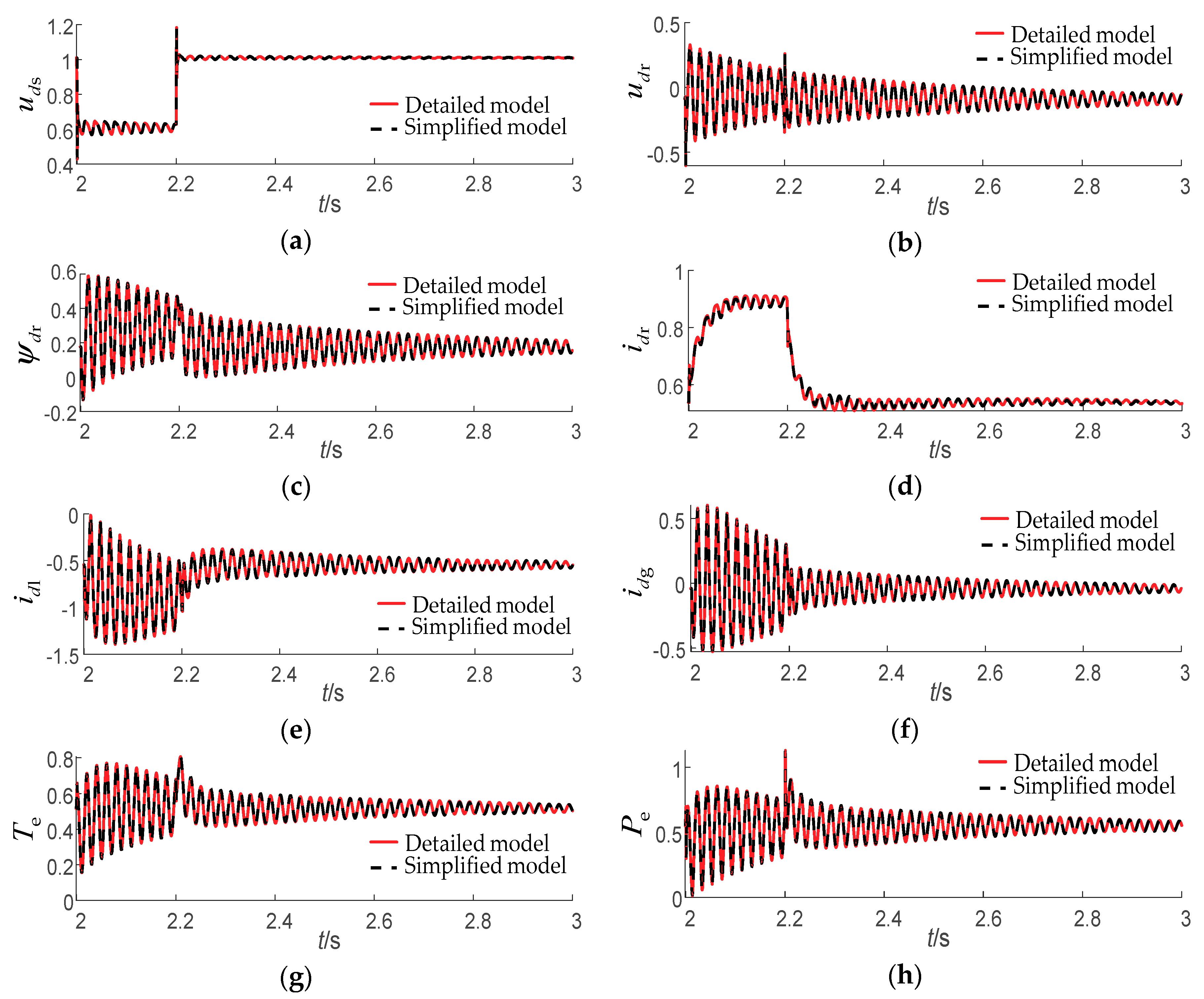
In the simulation, the initial wind speed is 10 m/s, and the wind turbine works at the MPPT stage. At t = 2 s, the wind speed mutates to 11 m/s. The dynamics of the detailed model and simplified models are shown in Figure 11 and Figure 12, where the electromagnetic transient process takes one frequency cycle after the disturbance, and the electromechanical transient simulation takes the time period of 30 s. Electrical variables recorded include: u_ds, u_dr, ψ_dr, i_dr, i_dl, i_dg, T_e, P_e, Q_e, and ω_r.

(1) Electromagnetic transient process

From Figure 11, it can be seen that at the disturbance of wind speed mutation, the dynamics of the variables in the electromagnetic transient time scale almost coincided with that of the detailed model. Therefore, it can be concluded that the established 14-order electromagnetic transient model can well simulate the dynamics of the detailed model in one frequency cycle, and thus, the rationality of the electromagnetic transient model is verified.

(2) Electromechanical transient process

From Figure 12, it can be seen that at the disturbance of wind speed mutation, the dynamics of the variables in the electromechanical transient process almost coincided with that of the detailed model. Therefore, it can be concluded that the established electromechanical transient model can well simulate the dynamics of the detailed model within 30 s and thus, the rationality of the electromechanical transient model is verified.

4.2. Simulations under Voltage Sag

Normally, the DFIG wind turbine system works at a wind speed of 10 m/s. At t = 2 s, a three-phase fault was introduced, and the PCC voltage dropped to 0.6 p.u; the fault was cleared and the voltage was restored to a normal level 0.2 s later.

It should be noted that the simulation analysis in this paper does not take into account the effects of nonlinear links such as amplitude limiting. At the moment of voltage sag, the control system will make the electromagnetic power return to the power reference value in a short time, which means that the mechanical torque and the electromagnetic torque can quickly reach the balance, and the impact on the rotor speed is relatively small.

(1) Electromagnetic transient process

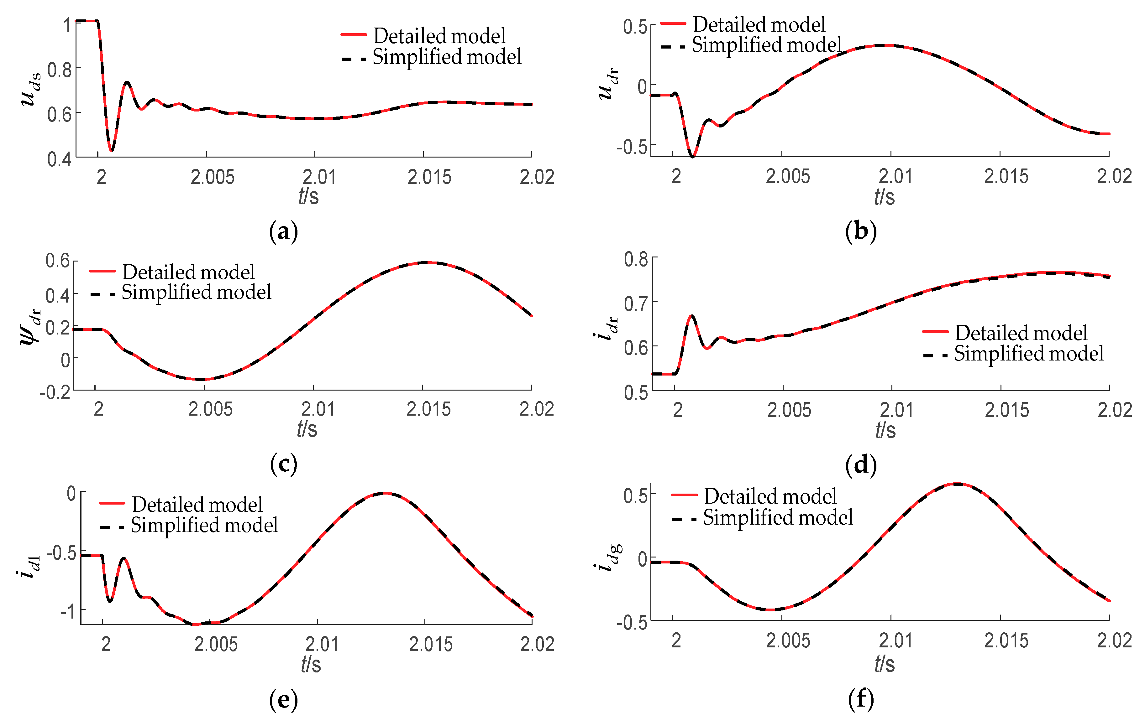
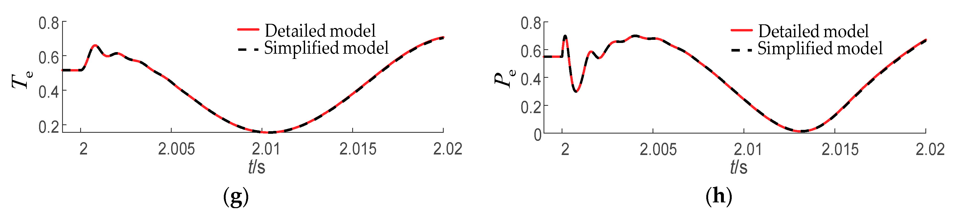
Based on the 14-order electromagnetic transient model, the simulation results are compared with the detailed models. The dynamics during voltage sag are shown as in Figure 13, while the dynamics in one frequency cycle are shown as in Figure 14. In the figures, the electrical variables recorded include: u_ds, u_dr, ψ_dr, i_dr, i_dl, i_dg, T_e, P_e, and ω_r.

From Figure 13 and Figure 14, it can be seen that at the disturbance of voltage, the dynamics of the variables in the electromagnetic transient process almost coincided with those of the detailed model. Therefore, it is proved that the electromagnetic transient model can fully simulate the overall dynamics of the DFIG wind turbine system, the electromagnetic transient model is valid, and the analysis of the order-reduction process is rational.

In order to observe the dynamics of the generator rotor speed, the electromechanical transient model is used to simulate the working condition, and the detail is given in the electromechanical transient process simulation.

(2) Electromechanical transient process

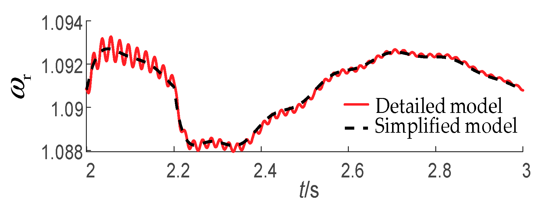
In the 12-order electromechanical transient model of Table 8, the dynamics of the PLL are taken into account without consideration of the dynamics of the stator-side energy storage element. As a result, the q-axis voltage of the stator in the simulation is greatly deviated at the moment of voltage sag, which makes the PLL output angular frequency produce a big error, and leads to the collapse of the DFIG wind turbine system. Therefore, the 10-order electromechanical transient model corresponding to Table 7 is adopted for electromechanical simulation by neglecting the PLL dynamics of the 12-order electromechanical transient model.

In the 10-order model, the equilibrium point of the electrical variables shifted according to that of the 12-order model. However, as the attenuation time of the electrical variables is much smaller than that of the mechanical variables, the dynamic characteristics of the mechanical variables are hardly affected. Therefore, the 10-order model of Table 7 can be used to observe the dynamics of the rotor speed. The dynamics of the rotor speed in the 26-order detailed model, as well as those in the 10-order model, are shown in Figure 15, and the result verifies the effectiveness of the 10-order model.

4.3. Summary

From the perspective of simulation accuracy, the 14-order electromagnetic model and 12 or 10-order electromechanical model can accurately demonstrate the dynamics of the detailed model no matter whether they are under wind speed mutation or voltage sag disturbance. From the perspective of simulation speed, the simulation speed of the model can be indicated by the order of the differential equations. Compared with the 26-order detailed model, the simplified models have significant reduction in the order of the model, and thus have greatly improved the simulation speed. Moreover, considering that the variables of the electromechanical model change relatively slowly, the sampling time of the electromechanical model can be increased in order to further improve the simulation speed of the model.

5. Conclusions

In this paper, the multi-time scale characteristics of the DFIG wind turbine system were explained by constructing the small disturbance model with the equilibrium point at the MPPT stage. The proposed electromagnetic transient model and electromechanical transient model of the DFIG wind turbine system were obtained respectively by taking the variation in the eigenvalues of the DFIG wind turbine system before and after the order reduction as the initial rationality criterion for model reduction, and analyzing the coupling between variables and the system, as well as the coupling between the variables of different time scales. The validity of the simplified models were verified by simulation in the case of large disturbances.

The conclusions are as follows:

(1)

Ignoring the integral part of the inner loop controller of the dual PWM converter control system has little effect on the eigenvalues of the model.

(2)

According to the time-scale distribution of the variables, ignoring the variables that have large differences with the time scale of the transient process, the order of the system model can be reduced. However, the eigenvalue distribution of the simplified model may be quite different from that of the detailed model. The reason is that the reduced-order method based on the time-scale distribution of variables ignores the coupling between variables, as well as the coupling between variables and systems in the transient process of the actual system.

(3)

In both the small disturbance analysis and the large disturbance simulation, the 14-order electromagnetic transient model that is presented in this paper can well represent the dynamics of the detailed model in the time scale of the electromagnetic transient process, and achieves a balance in simulation speed and accuracy.

(4)

As to the 10-order electromechanical transient model presented in this paper, the ignorance of the dynamics of the PLL makes the equilibrium point of the model deviate under disturbance, but does not affect the dynamic trend of mechanical variables. Meanwhile, the 12-order electromechanical transient model of this paper takes into account the dynamics of the PLL and improves the simulation accuracy of the model, but it is not suitable for the analysis of voltage sag conditions.

(5)

It is also possible to use the simplified models of other orders mentioned in this paper according to the actual working conditions.

In the future, on the basis of the simplified models proposed in this paper, the authors will further explore the mechanism of stability problems related to large-scale wind power connecting to the power grid, and study the strategies to improve the stability of wind power grid-integrated system so as to enhance the wide use of wind power.

References

- Han, P.P.; Lin, Z.H.; Wang, L.; Fan, G.J.; Zhang, X.A. A survey on equivalence modeling for large-scale photovoltaic power plants. Energies 2018, 11, 1463. [Google Scholar] [CrossRef]
- Global Wind Energy Council. Global Wind Report. Available online: http://files.gwec.net/files/GWR2017.pdf (accessed on 20 October 2018).
- Ding, M.; Zhang, Y.; Han, P.P.; Bao, Y.Y.; Zhang, H.T. Research on optimal wind power penetration ratio and the effects of a wind-thermal-bundled system under the constraint of rotor angle transient stability. Energies 2018, 11, 666. [Google Scholar] [CrossRef]
- Xiang, Y.; Sun, X.Q.; Zhang, X.Q.; Duan, N.X. The problems exposed in the accident of a large number of wind power generators get offline on feb 24th 2011 in gansu and the solutions. North China Elec. Power 2011, 9, 1–7. [Google Scholar] [CrossRef]
- Fan, G.F.; Pei, Z.Y.; Xiao, Y.; Wang, N.B.; Zhang, S. Research on response speed and it’s test method of reactive power compensation equipment in wind farm. Smart Grid 2015, 3, 139–144. [Google Scholar] [CrossRef]
- Wind Farm—DFIG Detailed Model. Available online: http://cn.mathworks.com/help/physmod/sps/examples/wind-farm-dfig-detailed-model.html?searchHighlight=DFIG&s_tid=doc_srchtitle (accessed on 20 October 2018).
- Ting, L.; Barnes, M.; Ozakturk, M. Doubly-fed induction generator wind turbine modelling for detailed electromagnetic system studies. IET Renew. Power Gener. 2013, 7, 180–189. [Google Scholar] [CrossRef]
- Song, G.B.; Zhang, C.H.; Wang, X.B.; Huang, W. Simplified method of doubly fed induction generator. J. Eng. 2017, 2017, 1200–1205. [Google Scholar] [CrossRef]
- Xu, Z.; Pan, Z.P. Influence of Different Flexible Drive Train Models on the Transient Responses of DFIG Wind Turbine. In Proceedings of the 2011 International Conference on Electrical Machines and Systems, Beijing, China, 20–23 August 2011. [Google Scholar]
- Xu, Y.; Chen, L.; Chen, Y.; Sun, Z.Q. A fast transient simulation model of the DFIG based on the switching-function model of the VSC. In Proceedings of the 2012 International conference on Power system Technology, Auckland, New Zealand, 30 October–2 November 2012. [Google Scholar]
- Lei, H.Y.; Zhang, C.; Wang, N.B.; Ma, S.Y.; Zhao, C.Y.; Zhi, J. Equivalent simulation of doubly-fed induction generators based on controlled source models of converters. Elec. Power 2012, 45, 82–87. [Google Scholar]
- Li, J.; Wang, W.S.; Song, J.H. Simplified dynamic model of doubly-fed induction generator and its application in wind power. Elec. Power Autom. Equip. 2005, 25, 58–62. [Google Scholar]
- Zhao, M.Q.; Yuan, X.M.; Hu, J.B. Modeling of DFIG wind turbine based on internal voltage motion equation in power systems phase-amplitude dynamics analysis. IEEE Trans. Power Syst. 2018, 33, 1484–1495. [Google Scholar] [CrossRef]
- Zhang, B.Q.; Zhang, B.M.; Wu, W.C.; Zheng, Y.W. Time constant model analysis of double fed induction wind generator. In Proceedings of the International Conference on Electrical Engineering, Shenyang, China, 5 July 2009. [Google Scholar]
- Zhang, B.Q.; Zhang, B.M.; Wu, W.C. Small signal based reduced electromagnetic model analysis of double fed induction generator. Autom. Elec. Power Syst. 2010, 34, 51–55. [Google Scholar]
- Wang, Q.; Xue, A.C.; B, T.S.; Huo, J.D. A decomposed-reduced model based modes estimation method of DFIG. Power Syst. Prot. Control 2016, 44, 1–7. [Google Scholar] [CrossRef]
- Pan, X.P.; Ju, P.; Wu, F.; Jin, Y.Q. Discussion on model structure of DFIG-based wind turbines. Autom. Elec. Power Syst. 2015, 39, 7–14. [Google Scholar] [CrossRef]
- Wang, Y.J.; Hu, J.B.; Zhang, D.L.; Ye, C.; Li, Q. DFIG WT electromechanical transient behaviour influenced by PLL: Modelling and analysis. In Proceedings of the International Conference on Renewable Power Generation (RPG 2015), Beijing, China, 17–18 October 2015. [Google Scholar]
- Zhang, D.L.; Wang, Y.J.; Hu, J.B.; Ma, S.C.; He, Q.; Guo, Q. Impacts of PLL on the DFIG-based WTG’s electromechanical response under transient conditions: Analysis and modeling. CSEE J. Power Energy Syst. 2016, 2, 30–39. [Google Scholar] [CrossRef]
- Xie, D.; Feng, J.Q.; Lou, Y.C.; Yang, M.X.; Wang, X.T. Small-signal modelling and modal analysis of DFIG-based wind turbine based on three-mass shaft model. Proc. CSEE 2013, 33, 21–29. [Google Scholar] [CrossRef]
Figure 1.
Control block diagram of pitch angle.
Figure 2.
Model of the phase-locked loop (PLL).
Figure 3.
Control block diagram of rotor-side converter.
Figure 4.
Control block diagram of grid-side converter.
Figure 5.
Outline of model reduction process.
Figure 6.
Simplified control block diagram of the rotor-side converter.
Figure 7.
Simplified control block diagram of the grid-side converter.
Figure 8.
Dynamics of the rotor flux linkage: (a) The d-axis flux linkage of the rotor; (b) The q-axis flux linkage of the rotor.
Figure 9.
Distribution of variables in the detailed model and the simplified model.
Figure 10.
Grid connection structure of the DFIG wind turbine.
Figure 11.
Simulation of electromagnetic transient process under wind speed mutations (the solid line represents the result of the detailed model, and the dotted line represents the result of the 14-order electromagnetic transient model): (a) uds; (b) udr; (c) ψdr; (d) idr; (e) idl; (f) idg; (g) Te; and (h) Pe.
Figure 12.
Simulation of electromechanical transient process under wind speed mutations (the solid line represents the result of the detailed model, and the dotted line represents the result of the 12-order electromagnetic transient model): (a) uds; (b) udr; (c) ψdr; (d) idr; (e) ωr; (f) idg; (g) Qe; and (h) Pe.
Figure 13.
Simulation of electromagnetic transient process under voltage drop conditions (the solid line represents the result of the detailed model, and the dotted line represents the result of the 14-order electromagnetic transient model): (a) uds; (b) udr; (c) ψdr; (d) idr; (e) idl; (f) idg; (g) Te; and (h) Pe.
Figure 14.
Electromagnetic transient local process simulation under voltage drop conditions (the solid line represents the result of the detailed model, and the dotted line represents the result of the 14-order electromagnetic transient model): (a) uds; (b) udr; (c) ψdr; (d) idr; (e) idl; (f) idg; (g) Te; and (h) Pe.
Figure 15.
Trend of generator speed under voltage drop conditions (the solid line is the detailed model, and the dotted line is the 10-order electromechanical transient model).