Numerical Study of the Magnetic Field Effect on Ferromagnetic Fluid Flow and Heat Transfer in a Square Porous Cavity


1
College of Engineering, Effat University, 21478 Jeddah, Saudi Arabia
2
Department of Mathematics, Faculty of Science, Aswan University, Aswan 81528, Egypt
3
Department of Electrical Engineering, College of Engineering, King Saud University, P.O. Box. 800, 11421 Riyadh, Saudi Arabia
4
Department of Electrical Engineering, Faculty of Energy Engineering, Aswan University, Aswan 81528, Egypt
5
Ecole Centrale de Lyon, University of Lyon, AMPERE CNRS UMR 5005, 36 Avenue Guy de Collongue, 69134 Ecully, France
*
Author to whom correspondence should be addressed.
Energies 2018, 11(11), 3235; https://doi.org/10.3390/en11113235
Submission received: 12 August 2018
/
Revised: 25 October 2018
/
Accepted: 19 November 2018
/
Published: 21 November 2018
(This article belongs to the Special Issue Fluid Flow and Heat Transfer)
Abstract
:A numerical study of ferromagnetic-fluid flow and heat transfer in a square porous cavity under the effect of a magnetic field is presented. The water-magnetic particle suspension is treated as a miscible mixture and, thus, the magnetization, density and viscosity of the ferrofluid are obtained. The governing partial-differential equations were solved numerically using the cell-centered finite-difference method for the spatial discretization, while the multiscale time-splitting implicit method was developed to treat the temporal discretization. The Courant–Friedrichs–Lewy stability condition (CFL < 1) was used to make the scheme adaptive by dividing time steps as needed. Two cases corresponding to Dirichlet and Neumann boundary conditions were considered. The efficiency of the developed algorithm as well as some physical results such as temperature, concentration, and pressure; and the local Nusselt and Sherwood numbers at the cavity walls are presented and discussed. It was noticed that the particle concentration and local heat/mass transfer rate are related to the magnetic field strength, and both pressure and velocity increase as the strength of the magnetic was increased.
1. Introduction
Ferromagnetic fluids are smart fluids [1,2], composed of magnetized nanoparticles suspended in a liquid-based medium, such as oil and water. Ferromagnetic fluids have been used in different engineering and environmental applications, such as enhanced oil recovery (EOR). The idea of using ferrofluids, such as iron oxide, Fe2O3, and zinc oxide, ZnO, under an external magnetic field is to control the ferrofluids’ movement in porous media [3,4,5]. Heat transfer in porous media involves a wide range of applications such as heat exchangers, oil/gas recovery, geophysical systems, nuclear waste disposal, chemical reactors, thermal insulation of buildings, and drying processes. Chegenizadeh et al. [6] provided a classification of the most popular nanoparticles under optimal operational conditions. El-Amin et al. [7,8] conducted some studies on modeling nanoparticle transport in porous media. Suleimanov et al. [9] and Ryoo et al. [10] conducted an experimental investigation of using nanoparticles in enhanced oil recovery application.
Flows in cavities have many technological applications, such as heat exchangers, cooling systems for electronic equipment, and environmental flows. Sheremet and Pop [11] investigated the steady laminar mixed convection inside a lid-driven square cavity filled with a water-based nanofluid. Chalambaz et al. [12] studied the heat and mass transfer in a square porous cavity with differential temperature and concentration at the sidewalls, and they found that the heat transfer of the mixture and the mass transfer of the other phase can be maximized for specific values of the Lewis number of one phase. Carvalho and de Lemos [13] presented the problem of laminar free convection within a square porous cavity filled with a saturated fluid. Javed et al. [14] presented a numerical study for free convection through a square enclosure filled with a ferrofluid-saturated porous medium under a uniform magnetic field.
Numerical simulation is an important tool enabling engineers and scientists to predict the transport phenomena, test, and optimize an appropriate intervention strategy for heat transfer [15]. The time-stepping method has been presented for the problems of fluid dynamics by using implicit-type time-marching procedures to resolve transients [16]. Martinez [17] solved the shallow water equations by using the time-splitting technique. The time viscosity-splitting method was used for the Boussinesq problem by Zhang and Qian [18]. A time-splitting Fourier spectral method has been developed for approximating singular solutions of the Gross–Pitaevskii equation [19]. El-Amin et al. [20,21,22,23] used a multiscale time-splitting strategy to manage different time-step sizes for different physics. In this research, a multiscale adaptive time-splitting scheme is introduced to simulate the problem of magnetic-field effects on ferrofluids and heat transfer with a single-phase flow in a porous cavity considering variation of the nanoparticle concentration.
2. Problem Definition
The problem of a single-phase flow with ferromagnetic fluid flow and heat transfer in a square porous cavity under the effect of an external magnetic field is considered in this study. The ferromagnetic fluids gain properties of both liquid and magnetized solid particles. If the ferromagnetic fluid is subjected to an external magnetic field, it flows toward the magnetic field, and the flow resistance increases. In the absence of the magnet, nearby ferrofluids act as normal liquid. Figure 1 shows the schematic diagram of the 2D square porous cavity of Cases 1 and 2. In Case 1, the cavity walls are kept at a low temperature/concentration, , except the inlet at the center of the left wall is kept at a higher temperature/concentration (Dirichlet boundary condition). Initially, the cavity was filled with a pure water, then the ferrofluid suspension injection begins. The flow boundary condition of the inlet is defined by the existing velocity, . Above and below inlet, the no-flow boundary condition, , is assumed, as circulation may exist close to the inlet. However, far away from the inlet region, the circulation is expected to vanish, and a constant pressure boundary condition, , is assumed. In Case 2, the walls are assumed adiabatic (), () as indicated in Figure 1b. The constant pressure, , is assumed to represent the flow boundary condition. The inlet is kept at high temperature, high concentration, , velocity . Above and below inlet are kept at low temperature concentration, , and no-flow () boundary condition.
3. Mathematical Modeling
The external permanent magnetic field produces attractive forces on the fluid. The external magnetic force with a variable concentration, and hence density, acts as a body force per unit volume, [4,24]:
where is the magnetic permeability. The specific volume, , is defined by:
Therefore, Equation (1) can be rewritten as:
Such that:
The quantities and may be approximated around the points (, which represent the non-magnetized case, as:
The magnetization M is a function of the magnetic field strength H:
The two parameters and depend on the type of the ferromagnetic material and controlled both the initial susceptibility and the saturation magnetization. Therefore, Equation (1) can be written as:
The resulting magnetic induction (B) is a sum of the magnetic field strength (H) and the magnetization (M), i.e., they are related by the following linear relationship:
Equation (5) is expressed in a scalar formulation, such that B, H, and M are scalars representing vector magnitudes. In this study, there is no free electric charge flow, so the Maxwell equations are reduced to the second Gauss law:
which means that the magnetic field induction is divergence-free. Ampere’s law is reduced to the form:
which means that the magnetic field is vorticity-free.
Assuming that the medium is free of ferromagnetic materials and a permanent magnet is the source of the magnetic field, we can use the simple Equations (8) and (9), to calculate the components of H directly [4]. This assumption decouples the calculation of the external magnetic field from the ferrofluid distribution. At a given location the gradient of H can be calculated by simple first-order differencing in each of the coordinate directions. The z-axis of the local magnet coordinate system is set perpendicular to the poles, and the magnet is located at the upper right corner as indicated in Figure 1. The flow simulation is in the x-y plane of the coordinate system (Equations (8) and (9) represent and in the x-axis and y-axis, respectively). The 2D magnetic field strength is given by [4]:
where is the distance between the poles of the magnet, and is the residual magnetization. If the ferromagnetic materials are heated to temperatures above the critical point (Curie temperature ), they become paramagnetic, whereas, below , spontaneous magnetization occurs. The Curie temperature for ferrofluids is high (e.g., for Fe2O3 is 948 K). The temperature dependence of the spontaneous magnetization at low temperatures, which is the case in this study, is given by Bloch’s law [25]:
where is the spontaneous magnetization at absolute zero. In fact, there are several other mechanisms of temperature influence on the resulting magnetization of the magnetic fluid. One of the most significant models is the Langevin model which takes into consideration the role of the thermal fluctuations of the magnetic moments of the particles. The Langevin model is considered one the simplest cases, which can be written as:
such that:
The thermal fluctuations of the magnetic moments are related to the Brownian diffusion by the second fluctuation-dissipation theorem, which will be ignored in this study for simplicity.
Combining Equations (10) and (13), one may write:
It is assumed that the volumes of pure water and ferrofluid are additive; therefore, the mixture density is defined as [4,24,26]:
where is the density of the pure water component, and is the density of ferromagnetic-particle component. The viscosity of the water–magnetic-particle mixture is calculated by the following linear relationship [4]:
where is the viscosity of the pure water. At a Reynolds number greater than 10, the inertial effect becomes significant. The inertial term, which is known as the Forchheimer term, can account for the nonlinear behavior of the pressure difference versus flow. Momentum conservation in porous media is represented by the extended non-Darcy’s law [27]:
where F is the inertia parameter, and is kinematic viscosity. In the above equation, the second term on the left-hand side represents the inertial term in Darcy’s equation. The magnetic field effect on the fluid flow acts as a body force in the extended Darcy’s law. Although this is an unsteady problem, however, the momentum (Darcy’s law) has no time derivative term which is experimentally based. Actual fluid velocity varies throughout the pore space, due to the connectivity and geometric complexity of that space. This variable velocity can be characterized by its mean or average value. The convective flows are caused by the temperature difference in terms of the Boussinesq approximation, in which the density of the body force term is calculated by:
The mass conservation equation is represented by:
The energy conservation equation in porous media can be represented as [23]:
The concentration (solute transport) equation may be represented as [26]:
In the above equations, is the concentration, is the initial concentration, is the heat capacity, D is the diffusion-dispersion tensor, is the gravitation acceleration, is the thermal conductivity of the fluid, hs is the thermal conductivity of the solid, is the permeability, is the temperature, is the initial temperature, is the fluid pressure, is the fluid velocity vector, is the thermal expansion coefficient, is the solute expansion coefficient, represents the porosity of the porous media, is the density of the fluid mixture, is the density of the solid phase, and is the fluid viscosity. Substituting Equation (16) into Equation (18), one may obtain:
Calculating the heat transfer rate at boundaries/surfaces within fluids is of great interest in industrial and technological applications. The Nusselt number (Nu), a dimensionless number, is the ratio of convective to conductive heat transfer across the boundary. Unlike in other studies in the literature, the local Nusselt number was calculated on the wall instead of the average Nusselt number, because it gives the direct heat transfer rate between the wall and the adjacent fluid. The local Nusselt number measures the competition between convection and conduction heat flows and is defined by:
where is the characteristic length; are the local surface heat fluxes and defined as:
where is the thermal conductivity of the fluid. Similarly, the local surface mass fluxes, maybe defined as:
Therefore, the local Sherwood number which represents the ratio of the convective mass transfer to the rate of diffusive mass transport and given by:
Initially, the cavity is filled with pure water and, then, the ferrofluid suspension injection begins. In the following, two cases based on the types of boundary condition are described:
Case 1. All the walls of the square cavity are kept cold at temperature and low concentration except that the center of the left wall is kept at a high temperature and a high concentration , as shown in Figure 1a. The boundary conditions are described mathematically as follows:
- at , , , , ,
- at inlet , , ;
- at , , , , ;
- at , , , , ;
- at , , , , ;
where refers to the injection location (inlet), and the velocity is taken to be zero on all cells (no-flow boundary conditions, i.e., impermeable wall) except for the central cells. The fluid exits from constant pressure boundary, , which is a kind of exit boundary, as it is smaller than the entire pressure.
Case 2. All the walls of the square cavity are adiabatic and isothermal with constant Dirichlet pressure, except that the center of the left wall is kept hot at temperature and high concentration . The upper and lower left walls are kept at a cold temperature and a low concentration with no-flow Neumann boundary condition (impermeable wall), as shown in Figure 1b. The boundary conditions are described mathematically as follows.
- at , , , , ,
- at inlet , , .
- at , , , , .
- at , , , , .
- at , , , , .
4. Numerical Method
The governing equations were discretized numerically using the CCFD method for the spatial discretization. The CCFD method is considered one of the most commonly used finite-difference methods for flow and transport in porous media, because it is locally conservative. In the CCFD method, one uses velocity on edges of the cell, and pressure on the center of the cell (cell-centered). The permeability is calculated using the harmonic averaging on the center as well.
The backward Euler time discretization was used for the time derivative of equations of temperature and concentrations, with a time-splitting implicit technique [17,20]. The outer time discretization, which had a relatively large time step, was used for pressure. The subscript represents the current time step, while the subscript represents the previous time step. The temperature and concentration had the same level of time discretization. The following procedures have been considered,
- -
- The total time interval, [0, T], is divided into a number of time steps, namely, , with a time-step of length .
- -
- For temperature and concentration, each interval, , was divided into a number of subintervals, i.e., .
- -
- The Courant–Friedrichs–Lewy stability condition (CFL < 1) is used to accomplish the time step-size adaptation.
- -
- The time-step size of the pressure was taken to be larger than the time-step sizes of temperature and concentration.
The algorithm can be stated as:
- -
- Calculating the pressure implicitly by coupling the continuity and momentum equations.
- -
- Compute the velocity explicitly.
- -
- Solve energy and concentration equations implicitly.
- -
- Update porosity, permeability, and density.
Now, let us express the pressure equation as:
The energy equation is computed implicitly as:
Similarly, the concentration equation is computed implicitly as:
In order to control the time-step size, the CFL condition (CFL < 1) is used. The CFL condition of the temperature and concentration equations is expressed as:
The numerical stability procedures can be summarized as follows:
- -
- The pressure time-step, is taken as an initial time step for both temperature and concentration equations.
- -
- After that, the conditions and are examined. If one of them is satisfied, the temperature/concentration time-step is divided into smaller steps.
- -
- Therefore, the conditions and are recalculated based on the new time steps and so on, until satisfying the conditions and .
5. Results and Discussion
To obtain physical insights, the system of the governing partial differential equations was solved numerically using the above numerical method. Two different cases were considered based on different boundary conditions, as in Figure 1a,b. In Case 1, all boundaries were of a Dirichlet type except that the west boundary was a no-flow boundary condition, which was a Neumann type. The physical and computational parameters are presented in Table 1. A value for the outer time loop k was selected, and the step size was determined; then, the time-step size was calculated based on the CFL conditions. In our calculation the velocity inlet was taken as m/s and the corresponding Reynolds number is 0.00143, which is suitable for flow in porous media.
Some error estimates are listed in Table 2 to examine the accuracy of the proposed scheme. The errors were calculated for temperature and concentration at various values of the time-step iteration, k. The results in Table 2 indicate that the error decreases as the number of time steps increases. In addition, the temperature error is very small and approaches zero; however, the concentration error needs bigger time step numbers to reach the desired approximation. Moreover, the calculated time step size () is plotted against its number m in Figure 2. Moreover, concentration profiles for different spatial grid size and of Case 1 are plotted in Figure 3 to show the grid independence test. The spatial discretization, , was chosen, respectively, as , , and . It is clear from Figure 3 that the differences between the three curves are very small, therefore, we choose the course grid, , for the computations in this study.
5.1. Results for Case 1
Figure 4a,b illustrates the temperature difference, , contours of Case 1 without the magnetic-field effect (Br = 0.0) and with the magnetic-field effect (Br = 1.2), respectively. It seems that the magnetic field slightly enhances the temperature. The differences between of the two cases are similar, and it seems to be hard to notice the small differences (around 1 K); however, the differences are shown clearly in Figure 5, which shows the temperature profiles against the x-axis at y = 1 m, for various values of Br of Case 1. In Figure 6, the concentration profiles are plotted against the x-axis at y = 1 m, for various values of Br of Case 1. It is clear from Figure 6 that as the parameter Br increases, the ferrofluid concentration increases.
The pressure and velocity magnitude () profiles are plotted in Figure 7a,b, respectively, against the x-axis at y = 1 m, for various values of Br of Case 1. These figures show that, as Br increases, pressure and velocity increase. The maximum differences are located in the inlet vicinity and gradually decrease far away from it.
In Figure 8, the local Nusselt numbers are plotted along the left wall, right wall, upper wall, and lower wall of the porous cavity, for various values of the parameter Br of Case 1. The magnetic field has no effect on the left wall because the advection effect is much larger than the magnetic effect. The variation in magnetic-field strength has a small effect on the other walls; however, the differences are clear. The higher local Nusselt number is located in the center of the left wall, which indicates that the heat transfer rate is high in that region. Moreover, the heat transfer rate on the right wall has high values around the center of the wall and decreases gradually in the edge closure. The negative sign indicates that the heat transfer direction is from the fluid to the solid wall. The behavior of the heat transfer rate on the upper wall is similar to that on the right wall, but the maximum heat transfer rate is shifted to the bottom edge. Finally, the local Nusselt number on the lower wall has maximum values close to the left portion and then decreases gradually near the edges.
Figure 9 illustrates the local Sherwood number profiles along the left-, right-, upper-, and lower-walls. It can be seen from this figure that the local Sherwood number profiles along the left and right walls are symmetric around the center of y-axis and they decrease gradually far away from the center toward the upper to the lower corners. The mass transfer rate on the left-wall is high close to the inlet region and decreases from bottom to top. The negative sign indicates that mass transfer direction is from the fluid to the solid wall. It also may be noticed that the mass transfer rate on the right-wall is very small. The local Sherwood number on the upper- and left-walls has a similar behavior and same order of magnitude with different signs. The local mass transfer rate has maximum values at .
In Figure 10, the transient temperature and concentration profiles are plotted against the x-axis at y = 4, at different times of the ferrofluid injections. It is interesting to observe from Figure 10a that the temperature reaches the steady-state after around 2 days of injection, while the concentration reaches its steady-state after 2000 days of injection as indicated in Figure 10b.
5.2. Results for Case 2
In Figure 11, the temperature profiles are plotted against the x-axis, for various values of Br of Case 2. This figure shows that the existence of the external magnetic field increases the temperature. The lowest temperature values are in the vicinity of the left wall, while the opposite happens at y = 2.5 m. The magnetic field has a small effect at the centerline as the advection dominates, whereas it has a clear effect far away from the high advection region (e.g., y = 1 m). As the parameter Br increases, the temperature increases, which may be interpreted as the magnetic field enhancing the kinetic energy, which, in turn, enhances the heat energy.
The concentration profiles are plotted in Figure 12 against the x-axis at y = 4 m, 2.5 m, for various values of Br of Case 2. At the centerline (y = 2.5 m), the concentration has maximum values close to the inlet and decreases gradually far away from the inlet, whereas then opposite is true at y = 4 m. The concentration has minimum values close to the left wall and increases gradually far away from it. As the magnetic field pulls the particles toward it based on its strength, the parameter Br increases the concentration of the ferrofluid.
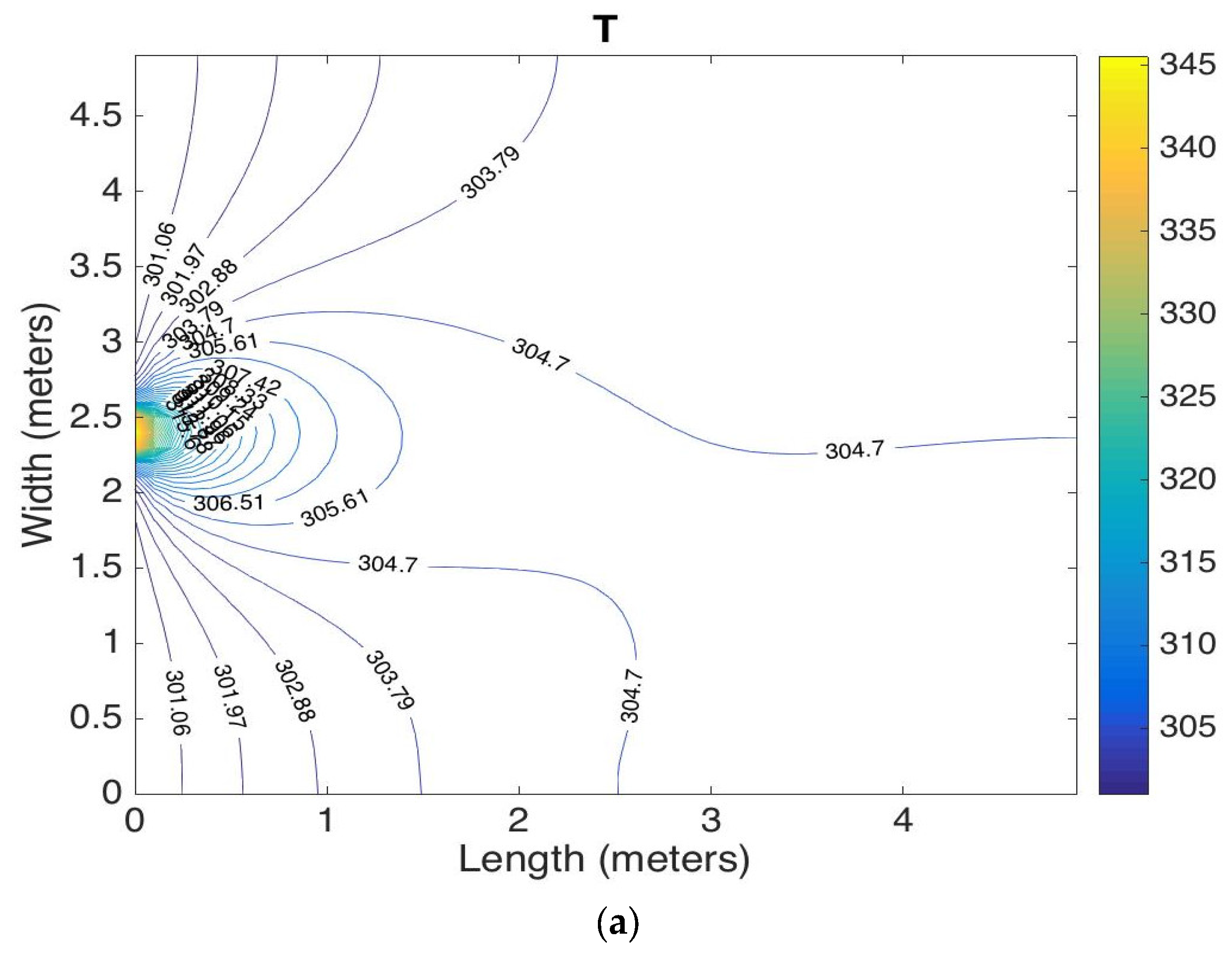
The temperature distribution of Case 2 is shown in Figure 13a. It can be seen from this figure that the temperature is high around the inlet location. Then it decreases gradually far away from the inlet because the other walls are adiabatic with a constant pressure. This may be interpreted as the heat transfer mode changes from the mixed convection region close to inlet to the purely conduction region far away. Figure 13b shows the concentration distribution of Case 2. The behavior of the concentration is similar to the temperature distribution which can be interpreted similarly but with respect to mass transfer and solute convection.
6. Conclusions
In this study, the effect of a magnetic field on ferromagnetic fluid flow and heat transfer in a square porous cavity was investigated. A mathematical model which consists of a set of governing equations and set of axillary algebraic equations, along with initial and boundary conditions, was developed. Two different cases of boundary conditions were considered. The governing equations were solved numerically using the multiscale time-splitting implicit method. An adaptive algorithm was built based on calculation of the Courant–Friedrichs–Lewy stability condition number. Error estimates for temperature and concentration at various values of iteration number were presented. Also, the grid independence of spatial discretization was examined. Numerical experiments were carried out to simulate some physical scenarios. It was found that the magnetic field increases the temperature and enhances the heat transfer rate. Also, the distribution of the particle concentration is related to the magnetic field strength. The pressure and velocity increase as the magnetic field strength increases. Close to the inlet the magnetic field had no effect on the local heat transfer rate because the advection force is much larger than the magnetic force. Moreover, the magnetic field strength had a small effect on the local heat transfer rate at the other cavity walls. The highest local Nusselt number occurs in the center of the left wall. Similar conclusions can be drawn for the mass transfer rate behavior under the effect of the magnetic field.
Author Contributions
Conceptualization, M.F.E., U.K. and A.B.; methodology, M.F.E. and U.K.; validation, M.F.E. and A.B.; analysis, M.F.E.; writing—original draft preparation, M.F.E.; writing—review and editing, M.F.E.; project administration, U.K.; funding acquisition, U.K.
Funding
This research was funded by the International Scientific Partnership Program (ISPP) at King Saud University, grant number ISPP#47.
Acknowledgments
The authors extend their appreciation to the International Scientific Partnership Program (ISPP) at King Saud University for funding this research work through ISPP#47. The authors also thank the Deanship of Scientific Research and RSSU at King Saud University for their technical support.
Conflicts of Interest
The authors declare no conflict of interest.
Nomenclature
| A | [m] | half of width of the magnet, |
| [A m−1] | constants depend on the type of the ferromagnetic material, | |
| b | [m] | half of height of the magnet, |
| [Tesla] | residual magnetization, | |
| [m m−3] | ferrofluid concentration, | |
| [m m−3] | ferrofluid initial concentration, | |
| [ | heat capacity, | |
| D | [m2 s−1] | diffusion coefficient, |
| [N] | external magnetic force, | |
| [m s−2] | gravitation acceleration, | |
| h | [ | thermal conductivity, |
| H | [A m−1] | magnetic field strength, |
| K | [m2] | permeability of the porous medium, |
| L | [m] | distance between the poles of the magnet, |
| Nu | [-] | Nusselt number, |
| [K] | temperature, | |
| [K] | reference temperature, | |
| [Pa] | fluid pressure, | |
| [kg s−1] | external mass flow rate, | |
| [ | rate of change of particle volume of a source/sink term, | |
| [ | heat source term, | |
| [ | fluid velocity vector, | |
| [m] | Cartesian coordinates, | |
| [K−1] | thermal expansion coefficient, | |
| solutal expansion coefficient, | ||
| [s] | time step for the loop k, | |
| [s] | time step for the loop l, | |
| [s] | time step for the loop m, | |
| [-] | porosity of porous media, | |
| [ | density of fluid mixture, | |
| [ | density of pure water component, | |
| [ | density of ferro-particles component, | |
| [ | density of solid phase, | |
| [m s−2] | viscosity of water-magnetic-particles mixture, | |
| [m s−2] | viscosity of water, | |
| [N A−2] | magnetic permeability. |
References
- Scherer, C.; Figueiredo Neto, A.M. Ferrofluids: Properties and applications. Braz. J. Phys. 2005, 35, 718–727. [Google Scholar] [CrossRef]
- Borglin, S.E.; Moridis, G.J.; Oldenburg, C.M. Experimental studies of the flow of ferrofluid in porous media. Transp. Porous Media 2000, 41, 61–80. [Google Scholar] [CrossRef]
- Huh, C.; Nizamidin, N.; Pope, G.A.; Milner, T.E.; Wang, B. Hydrophobic Paramagnetic Nanoparticles as Intelligent Crude Oil Tracers. U.S. Patent Application No. 14/765,426, 15 January 2014. [Google Scholar]
- Oldenburg, C.M.; Borglin, S.E.; Moridis, G.J. Numerical simulation of ferrofluid flow for subsurface environmental engineering applications. Transp. Porous Media 2000, 38, 319–344. [Google Scholar] [CrossRef]
- Zahn, M. Magnetic fluid and nanoparticle applications to nanotechnology. J. Nanopart. Res. 2001, 3, 73–78. [Google Scholar] [CrossRef]
- Chegenizadeh, N.; Saeedi, A.; Quan, X. Application of nanotechnology for enhancing oil recovery—A review. Petroleum 2016, 2, 324–333. [Google Scholar]
- El-Amin, M.F.; Salama, A.; Sun, S. Numerical and dimensional analysis of nanoparticles transport with two-phase flow in porous media. J. Pet. Sci. Eng. 2015, 128, 53–64. [Google Scholar] [CrossRef]
- El-Amin, M.F.; Salama, A.; Sun, S. Modeling and simulation of nanoparticles transport in a two-phase flow in porous media. In Proceedings of the SPE International Oilfield Nanotechnology Conference, Noordwijk, The Netherlands, 12–14 June 2012. SPE-154972-MS. [Google Scholar]
- Suleimanov, B.A.; Ismailov, F.S.; Veliyev, E.F. Nanofluid for enhanced oil recovery. J. Pet. Sci. Eng. 2011, 78, 431–437. [Google Scholar] [CrossRef]
- Ryoo, S.; Rahmani, A.; Yoon, K.Y.; Prodanovi, M.; Kots-mar, C.; Milner, T.E.; Johnston, K.P.; Bryant, S.L.; Huh, C. Theoretical and experimental investigation of the motion of multiphase fluids containing paramagnetic nanoparticles in porous media. J. Pet. Sci. Eng. 2012, 81, 129–144. [Google Scholar] [CrossRef]
- Sheremet, M.A.; Pop, I. Mixed convection in a lid-driven square cavity filled by a nanofluid: Buongiorno’s mathematical model. App. Math. Comput. 2015, 266, 792–808. [Google Scholar] [CrossRef]
- Ghalambaz, M.M.; Sheremet, F.; Mikhail, A.; Pop, I. Triple-diffusive natural convection in a square porous cavity. Transp. Porous Media 2016, 111, 59–79. [Google Scholar] [CrossRef]
- Carvalho, P.H.S.; de Lemos, M.J.S. Passive laminar heat transfer across porous cavities using thermal non-equilibrium model. Numer. Heat Transf. 2014, 66, 1173–1194. [Google Scholar] [CrossRef]
- Javed, T.; Mehmood, Z.; Abbas, Z. Natural convection in square cavity filled with ferrofluid saturated porous medium in the presence of uniform magnetic field. Phys. B Condens. Matter 2017, 506, 122–132. [Google Scholar] [CrossRef]
- Kleinstreuer, C.; Xu, Z. Mathematical modeling and computer simulations of nanofluid flow with applications to cooling and lubrication. Fluids 2016, 1, 16. [Google Scholar] [CrossRef]
- Bhallamudi, S.M.; Panday, S.; Huyakorn, P.S. Sub-timing in fluid flow and transport simulations. Adv. Water Res. 2003, 26, 477–489. [Google Scholar] [Green Version]
- Martinez, V. A numerical technique for applying time splitting methods in shallow water equations. Comput. Fluids 2018, 169, 285–295. [Google Scholar] [CrossRef]
- Zhang, T.; Qian, Y. The time viscosity-splitting method for the Boussinesq problem. J. Math. Anal. Appl. 2017, 445, 186–211. [Google Scholar] [CrossRef]
- Caliari, M.; Zuccher, S. Reliability of the time-splitting Fourier method for singular-solutions in quantum fluids. Comput. Phys. Commun. 2018, 222, 46–58. [Google Scholar] [CrossRef]
- El-Amin, M.F.; Kou, J.; Sun, S. Discrete-fracture-model of multi-scale time-splitting two-phase flow including nanoparticles transport in fractured porous media. J. Comput. Appl. Math. 2018, 333, 327–349. [Google Scholar] [CrossRef]
- El-Amin, M.F.; Kou, J.; Salama, A.; Sun, S. An iterative implicit scheme for nanoparticles transport with two-phase flow in porous media. Procedia Comput. Sci. 2016, 80, 1344–1353. [Google Scholar] [CrossRef]
- El-Amin, M.F.; Kou, J.; Sun, S.; Salama, A. Adaptive time-splitting scheme for two-phase flow in heterogeneous porous media. Adv. Geo-Energy Res. 2017, 1, 182–189. [Google Scholar] [CrossRef]
- El-Amin, M.F.; Kou, J.; Salama, A.; Sun, S. Multiscale adaptive time-splitting technique for nonisothermal two-phase flow and nanoparticles transport in heterogeneous porous media. In Proceedings of the SPE Reservoir Characterisation and Simulation Conference and Exhibition, Abu Dhabi, UAE, 8–10 May 2017. SPE-186047-MS. [Google Scholar]
- Rosensweig, R.E. Ferrohydrodynamics; Cambridge University Press: Cambridge, UK, 1985. [Google Scholar]
- Ashcroft, N.W.; Mermin, N.D. Solid State Physics; Holt, Rinehart and Winston: New York, NY, USA, 1976; ISBN 0-03-083993-9. [Google Scholar]
- Herbert, A.W.; Jackson, C.P.; Lever, D.A. Coupled groundwater flow and solute transport with fluid density strongly dependent upon concentration. Water Resour. Res. 1988, 24, 1781–1795. [Google Scholar] [CrossRef]
- El-Amin, M.F. Double dispersion effects on natural convection heat and mass transfer in non-Darcy porous medium. Appl. Math Comput. 2004, 156, 1–17. [Google Scholar] [CrossRef]
Figure 1.
Schematic diagram of the 2D square porous cavity—(a) Case 1: cavity walls are kept at a low temperature/concentration except the inlet at center of the left wall is kept at a higher temperature/concentration (Dirichlet boundary condition) and inlet velocity (Neumann boundary condition); (b) Case 2: the cavity walls are adiabatic and isothermal with constant pressure (Dirichlet boundary condition), except that the inlet at center of the left wall is kept at a high temperature/concentration and the upper/lower of left wall is kept at a low temperature/concentration with no-flow Neumann boundary condition. The z-axis of the local magnet coordinate system is set perpendicular to the poles, the x-y plane.
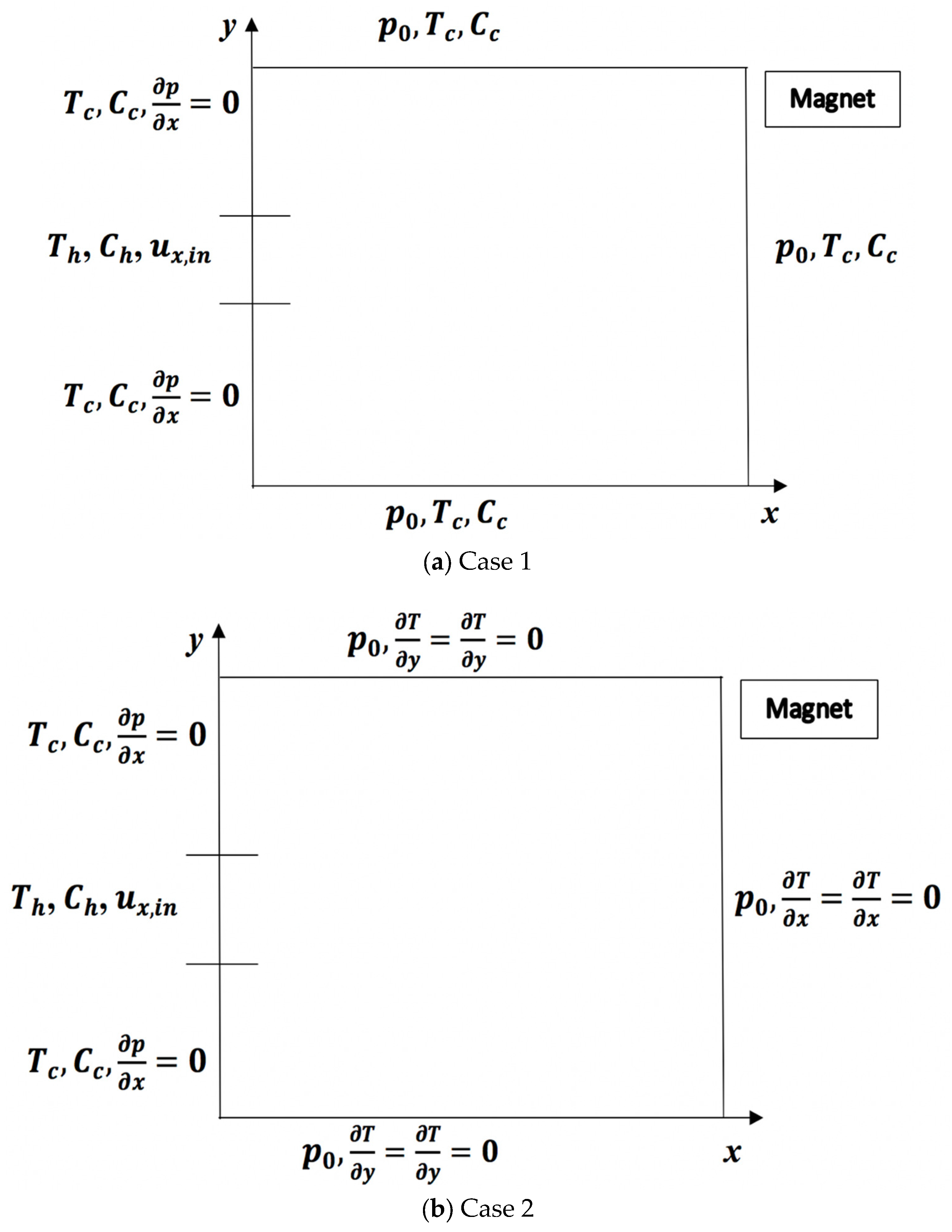
Figure 2.
Variation of the adaptive time step size () against its number m of Case 1.
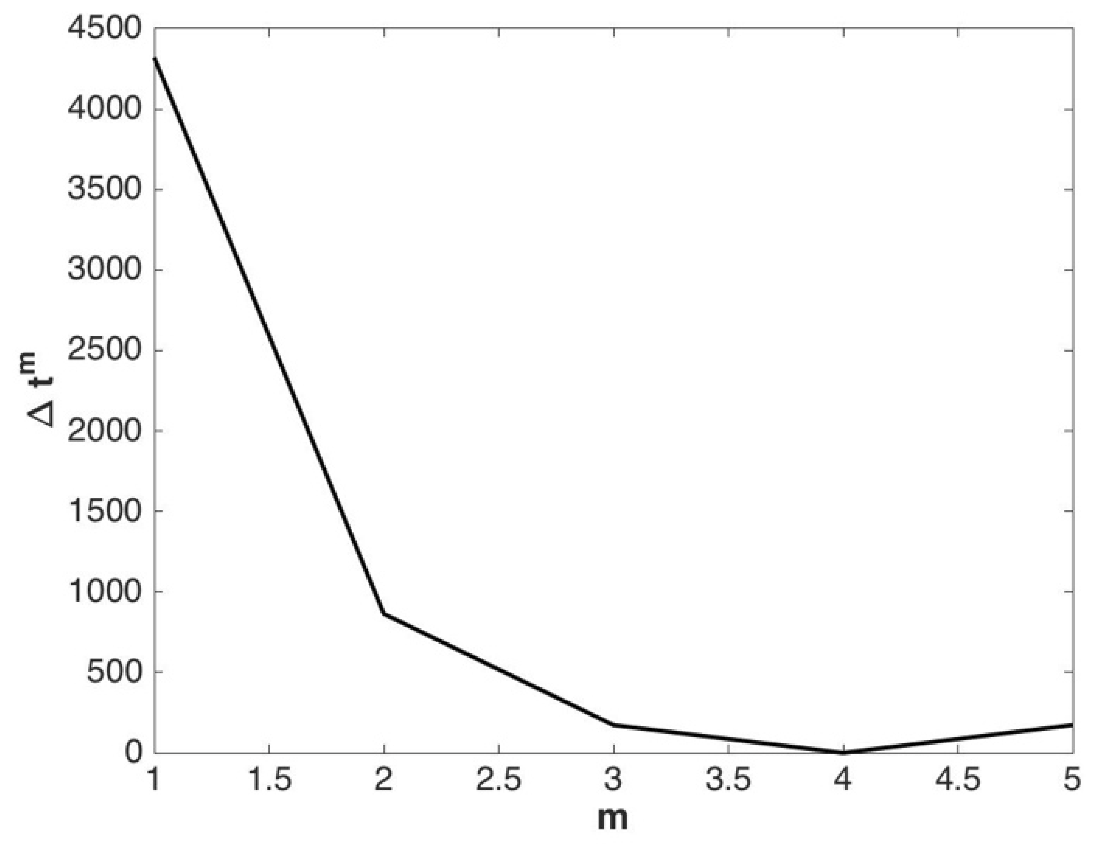
Figure 3.
Concentration profiles for different spatial grid size and of Case 1.

Figure 4.
Temperature difference, , contours of Case 1 with (a) Br = 0.0 and (b) Br = 1.2.
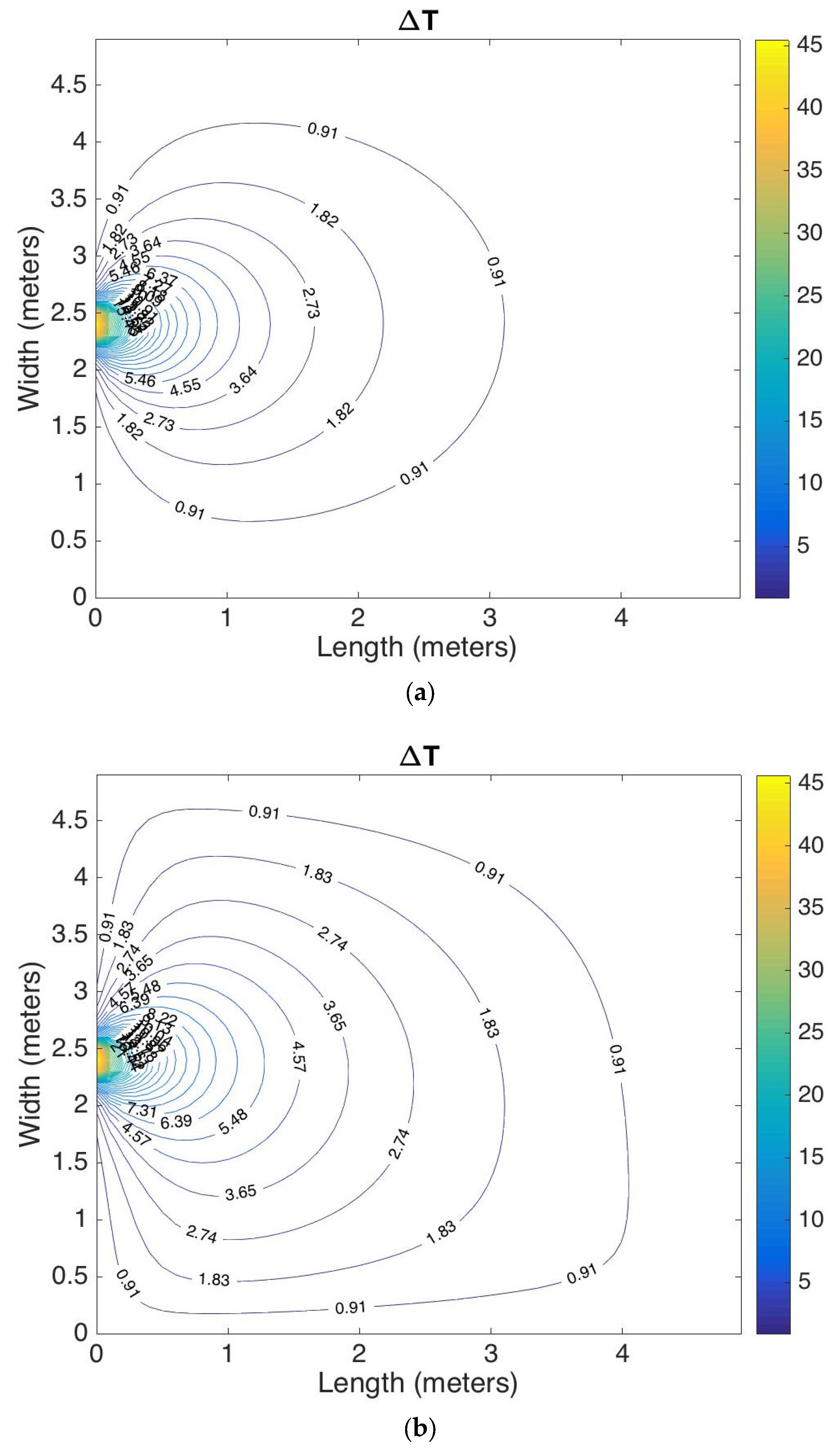
Figure 5.
Temperature profiles against x-axis at y = 1 m, for various values of Br of Case 1.
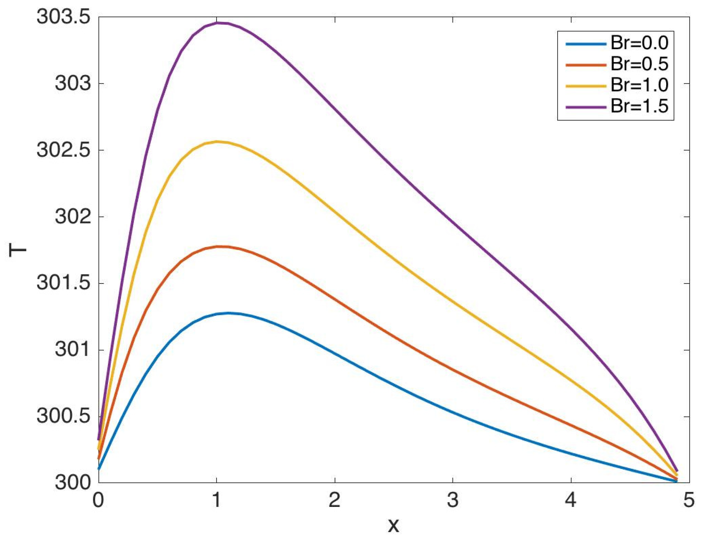
Figure 6.
Concentration profiles against the x-axis at y = 1 m, for various values of Br of Case 1.
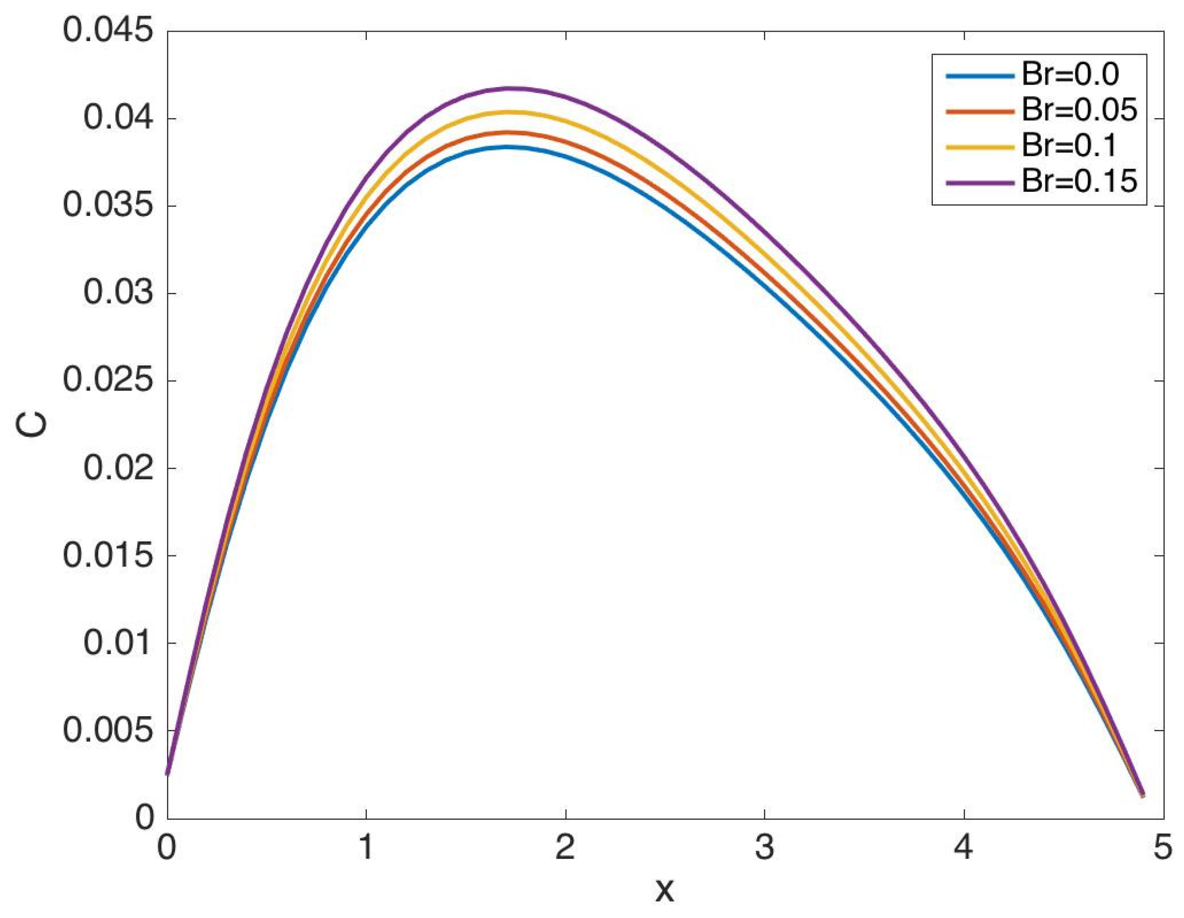
Figure 7.
(a) Pressure and (b) average velocity profiles against x-axis at y = 1 m, for various values of Br of Case 1.
Figure 7.
(a) Pressure and (b) average velocity profiles against x-axis at y = 1 m, for various values of Br of Case 1.
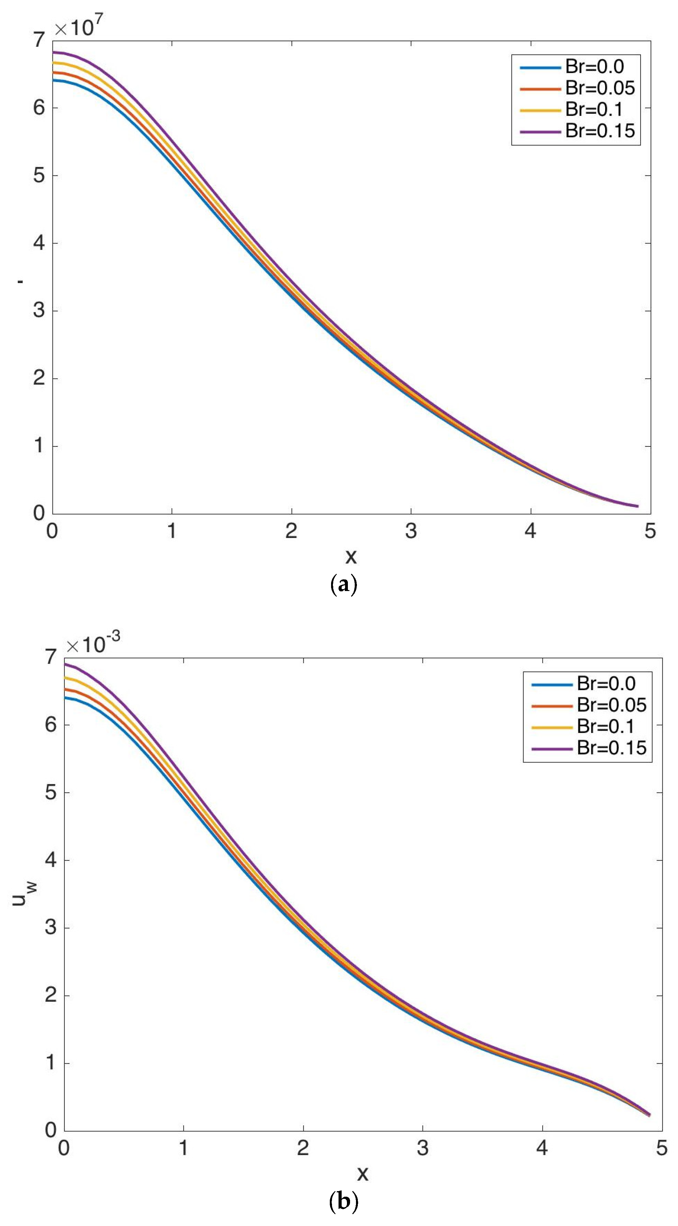
Figure 8.
Local Nusselt number distributions along the left wall, right wall, upper wall, and lower wall for various values of the parameter Br of Case 1.
Figure 8.
Local Nusselt number distributions along the left wall, right wall, upper wall, and lower wall for various values of the parameter Br of Case 1.
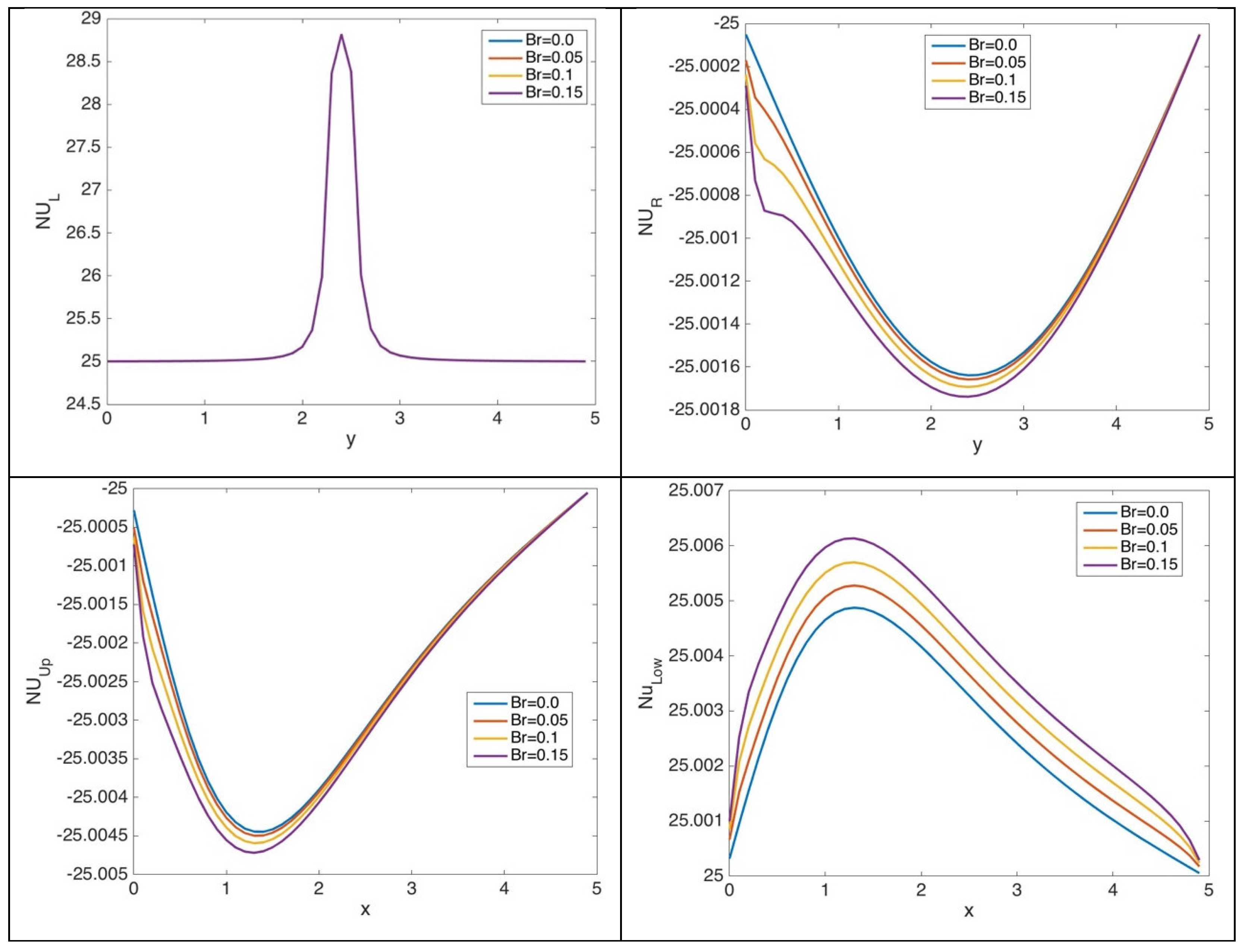
Figure 9.
Local Sherwood number profiles along the left-, right-, upper-, and lower-walls for various values of the parameter Br; Case 1.
Figure 9.
Local Sherwood number profiles along the left-, right-, upper-, and lower-walls for various values of the parameter Br; Case 1.
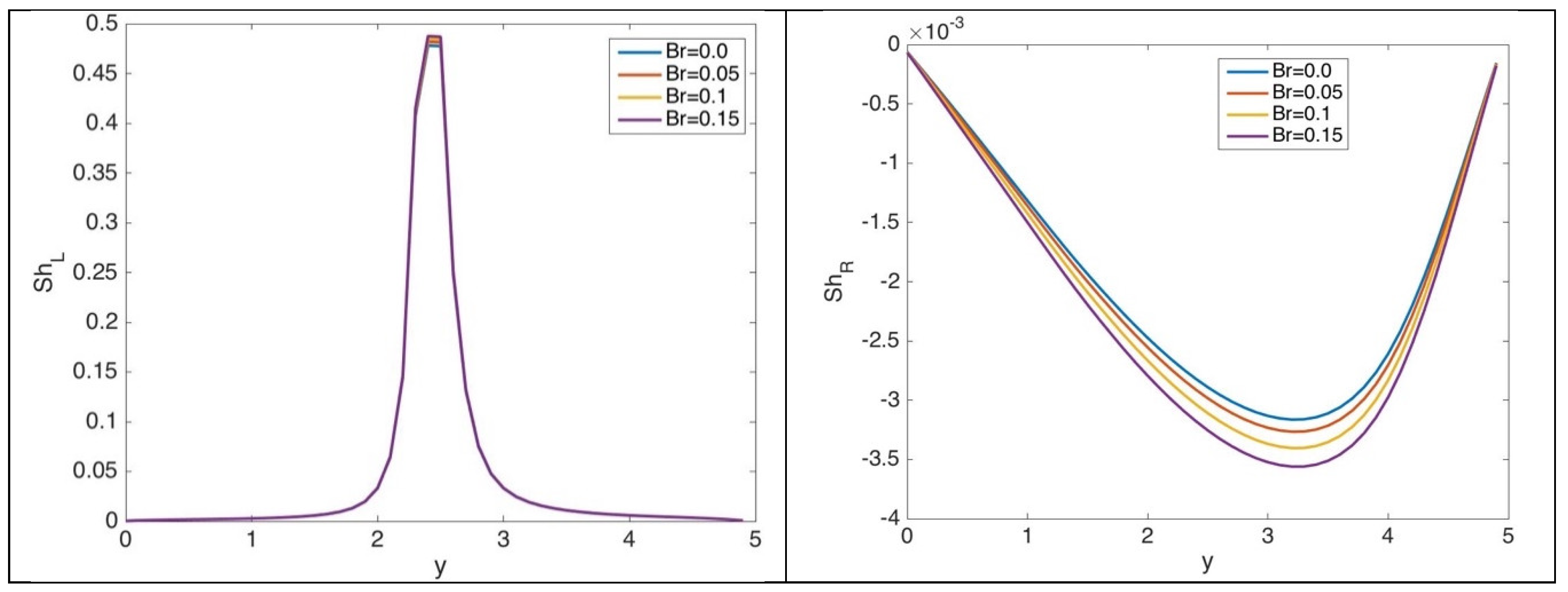
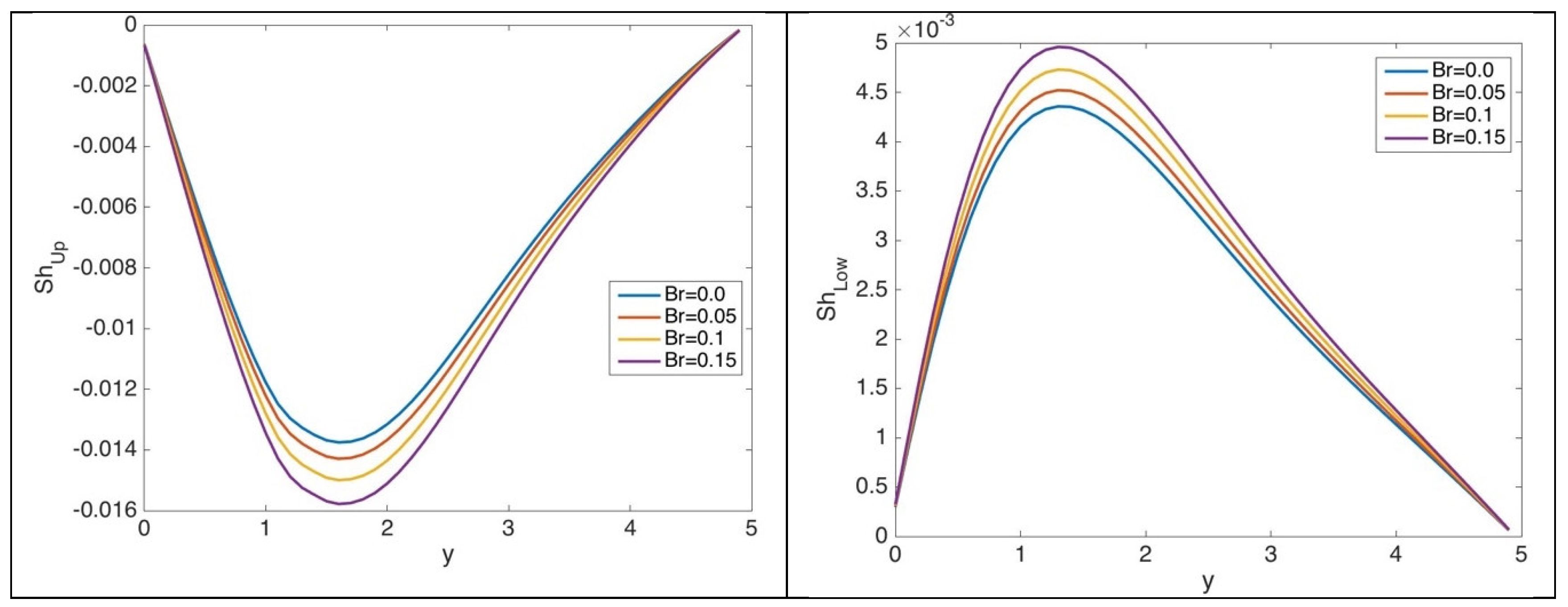
Figure 10.
Transient (a) temperature, and (b) concentration profiles against x-axis at y = 4, of Case 1.
Figure 10.
Transient (a) temperature, and (b) concentration profiles against x-axis at y = 4, of Case 1.
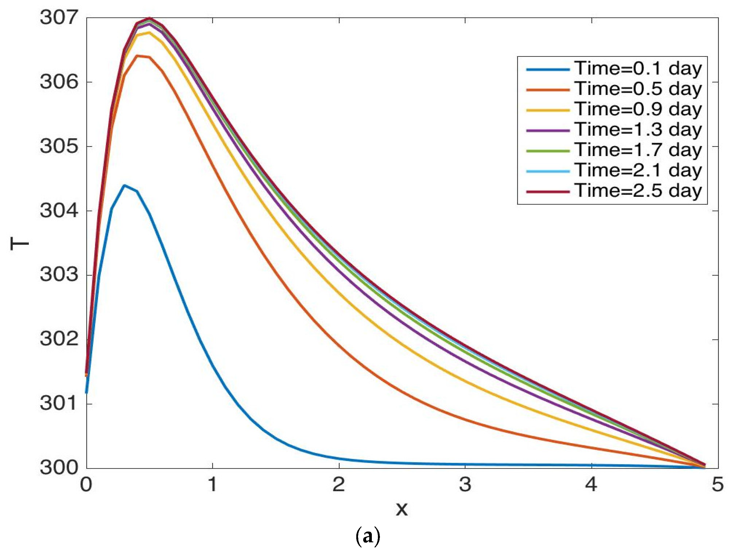
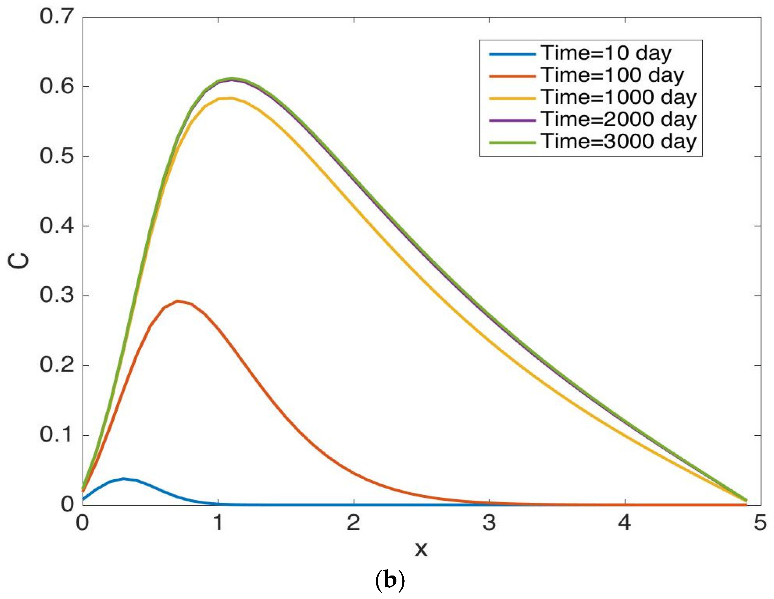
Figure 11.
Temperature profiles against x-axis at y = 1 m, 2.5 m for various values of Br of Case 2.
Figure 11.
Temperature profiles against x-axis at y = 1 m, 2.5 m for various values of Br of Case 2.

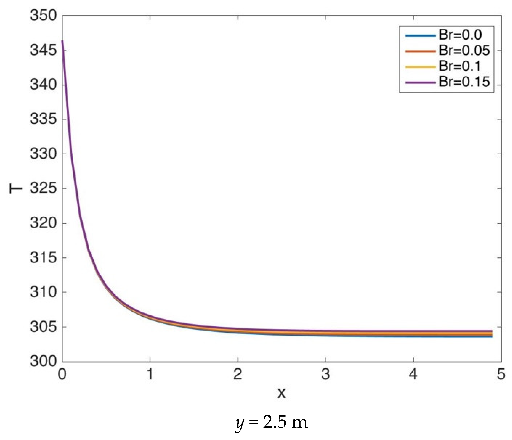
Figure 12.
Concentration profiles against x-axis at y = 4 m, 2.5 m, for various values of Br of Case 2.
Figure 12.
Concentration profiles against x-axis at y = 4 m, 2.5 m, for various values of Br of Case 2.
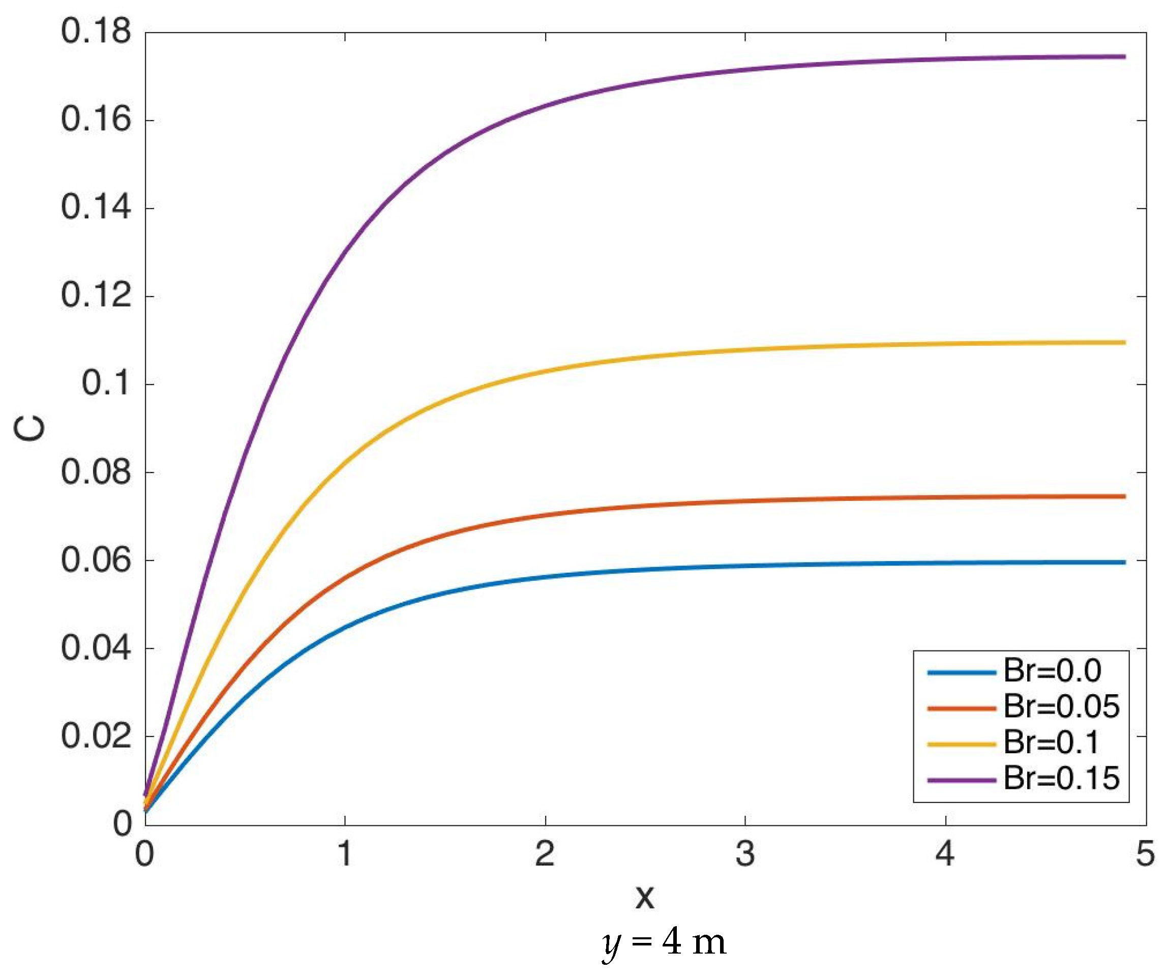
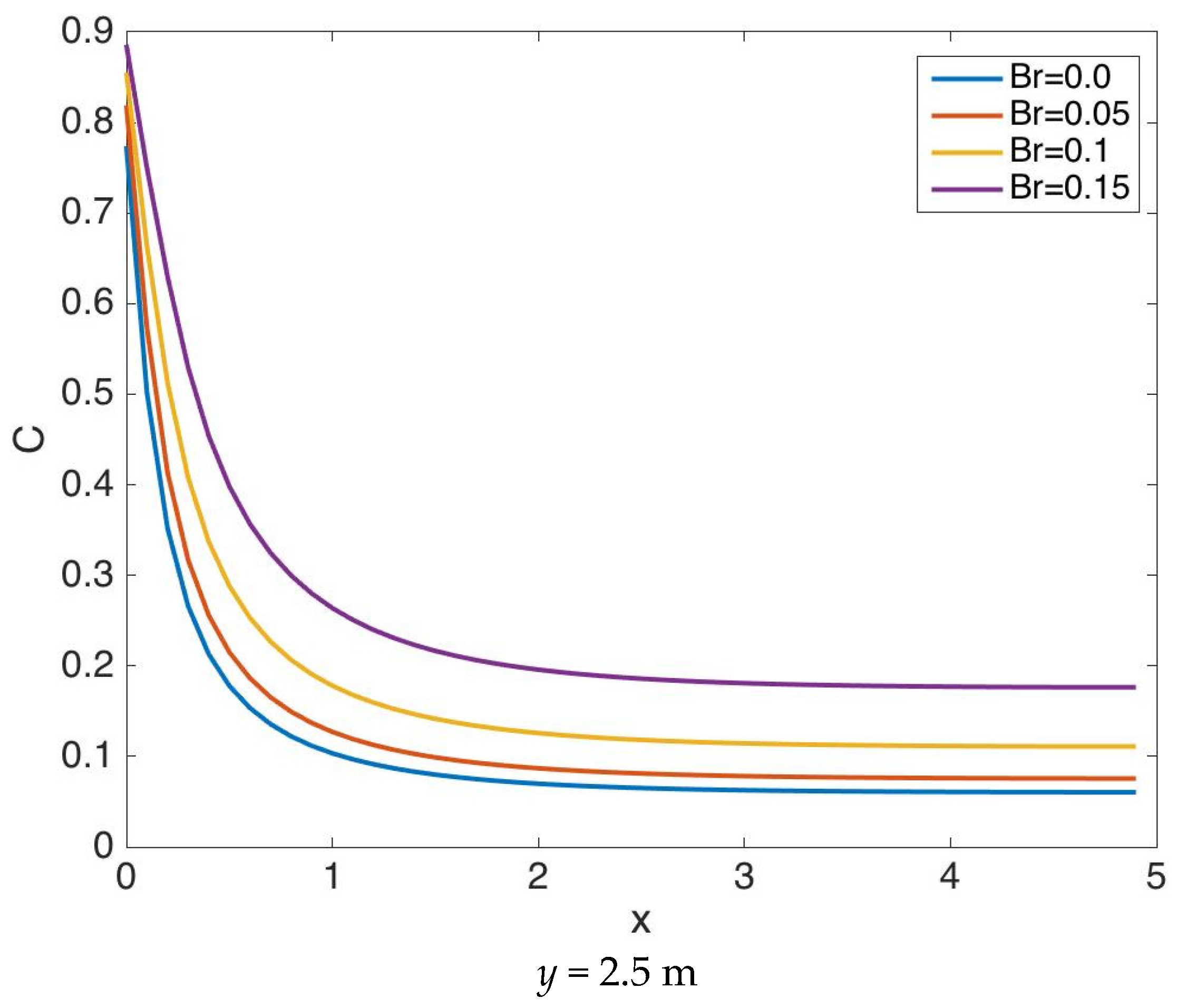
Figure 13.
Contours of (a) temperature, and (b) concentration, of Case 2.


Table 1.
Physical parameter values.
| Parameter | Description | Value | Units |
|---|---|---|---|
| Constant | 104–105 | m A−1 | |
| Constant | 10−6–10−5 | m A−1 | |
| a, b | Half of width/height of the magnet | 0.02 | m |
| Br | Residual magnetization | 0:0.2 | Tesla |
| Initial concentration | 0 | - | |
| Inlet concentration | 1 | - | |
| Heat capacity | 800 | J/Kg K | |
| D | Diffusion coefficient | 5 | /S |
| Thermal conductivity of the solid | 0.718 | W/(/K) | |
| Thermal conductivity of the ferrofluid | 0.6 | W/(/K) | |
| Gravity acceleration | 9.81 | ||
| K | Permeability | 100 | md |
| Lp | Distance between poles | 2.4 | m |
| Lin | Inlet width | 0.3 | m |
| L | Cavity side length | 5 | m |
| md | Millidarcy | 9.86923 | m2 |
| Initial pressure | 1 | ||
| Initial temperature | 300 | K | |
| Inlet temperature | 360 | K | |
| Inlet velocity | /s | ||
| Thermal expansion coefficient | 0.005 | ||
| Solute expansion coefficient | 0.001 | ||
| Porosity | 0.3 | - | |
| Water viscosity | 0.001 | Pa.s | |
| Magnetic permeability | 1 | N·A−2 | |
| Solid media density | 2500 | kg/ | |
| Pure water density | 1000 | kg/ | |
| Particles density | 8933 | kg/ |
Table 2.
Error estimates for various values of k, Case 2.
| k | ||
|---|---|---|
| 50 | 5.0317 × 10⁻¹¹ | 0.0198 |
| 100 | 6.9070 × 10⁻¹¹ | 0.0099 |
| 300 | 3.0481 × 10⁻¹² | 0.0033 |
© 2018 by the authors. Licensee MDPI, Basel, Switzerland. This article is an open access article distributed under the terms and conditions of the Creative Commons Attribution (CC BY) license (http://creativecommons.org/licenses/by/4.0/).
Share and Cite
MDPI and ACS Style
El-Amin, M.F.; Khaled, U.; Beroual, A. Numerical Study of the Magnetic Field Effect on Ferromagnetic Fluid Flow and Heat Transfer in a Square Porous Cavity. Energies 2018, 11, 3235. https://doi.org/10.3390/en11113235
AMA Style
El-Amin MF, Khaled U, Beroual A. Numerical Study of the Magnetic Field Effect on Ferromagnetic Fluid Flow and Heat Transfer in a Square Porous Cavity. Energies. 2018; 11(11):3235. https://doi.org/10.3390/en11113235
Chicago/Turabian StyleEl-Amin, Mohamed F., Usama Khaled, and Abderrahmane Beroual. 2018. "Numerical Study of the Magnetic Field Effect on Ferromagnetic Fluid Flow and Heat Transfer in a Square Porous Cavity" Energies 11, no. 11: 3235. https://doi.org/10.3390/en11113235
Note that from the first issue of 2016, this journal uses article numbers instead of page numbers. See further details here.