Abstract
The research of a general methodology to predict the pump performance in a reverse mode, knowing those of a pump in a direct mode, is a question that is still open. The scientific research is making many efforts toward answering this question, but at present, there is still not much clarity. This consideration has been the starting point of this research that thanks to artificial neural networks and evolutionary polynomial regression methods have tried to investigate and define the real weight of every input parameter, representing the efficiency of a pump in a direct way, on the output parameters, and representing efficiency of a pump used like a turbine.
1. Introduction
Electric vehicles (EVs), as an alternative to fuel vehicles (FVs), are considered zero emission cars. This statement is actually a half-truth; in fact, while EVs drastically reduce polluting emissions, more EVs will require more and more energy and the question becomes: how will this energy be produced? The European Environment Agency (EEA) [1] has tried to make assumptions about the future number of EVs and what their impact could be. In an optimistic scenario, the percentage of EVs by 2050 will be 80%; however, in a more realistic scenario, EVs in 2050 will represent half of the vehicles in circulation. It is only a hypothesis, but in future, EVs will be widespread and governments, even if the times remain unknown, will have to face the following problem: the FVs will be replaced by EVs and the electricity demand will increase very fast.
The future road transport and electric power sectors will become more closely linked if there is a wide uptake of electric vehicles in the European Union (EU). Recent findings from the EEA show that, if a hypothetical 80% of cars in 2050 will be electric, an additional 150 GW of additional electricity generation capacity would be needed across the EU. The risk, however, is that despite the great advance in mobility, global emissions will not drop and pollution will double. If most world governments, in fact, will keep relying on fossil fuel, the problem of pollution will shift from cars to power plants. The European Environment Agency suggests covering the additional 150 GW required by the advanced scenario for powering EVs with renewable energies with the following subdivision: 87 GW from wind power, 45 GW from photovoltaic, 24 GW from hydropower, and 13 GW from biomass [1].
The last statement highlights a very interesting question in terms of water resources because the hydropower generation, which is probably the oldest renewable energy source [2], is nowadays extensively exploited and the energy produced is already sent into the electric grid. Hydropower is already a mature technology in Europe, with an estimated total installed capacity of 294 GW [3]. Most of the hydropower potential is developed in northern Europe and alpine regions; in particular, Italy already has an installed hydropower capacity of 21.9 GW; however, most of the unutilized potential is concentrated in eastern Europe. Today the majority of investments in Europe are concerned with the renovation of existing facilities to minimize environmental impacts, improve efficiency, flexibility, and system resilience.
However, if on one hand the large- and medium-hydroelectric sector has been exploited extensively, and at the same time, the potential reduction of water resources due to extensive agriculture and drinking water demand grows, on the other hand small-, mini-, and micro-hydropower may represent an optimal and useful solution to produce energy from small water streams supplying rural centers and hilly areas. An interesting opportunity is represented nowadays by the energy recovery from water distribution networks (WDNs) converting water pressure in excess into electric energy or using hydraulic jumps in open channels.
Pressure control is one of the most important issues in optimizing the operation of WDNs [4]. Currently, a common practice that aims to control and reduce leakages involves the installation of pressure reduction valves (PRVs) in those points of the WDN where the pressures are high. A novel approach consists of installing pumps-as-turbines (PATs) or replacing PRVs already installed into the WDN and producing significant amount of energy converting water pressure into electric energy. Undoubtedly, the flow rate and water pressure are extremely variable at every point of a WDN; however, there are nodes of the network whose elevation is the lowest of the surrounding nodes, where often the pressure is greater than necessary. Technical literature summarized several examples about PAT devices in a real aqueduct or WDN: Muhammetoglu et al. [5] reported the results of a PAT system installed on a by-pass line of the Antalia (Turkey) WDN and demonstrated how the system is able to produce energy between 0.7 and 7 kWh. Rossi et al. [6] selected the optimal PAT to insert into the aqueduct of Merano, a town located in South-Tyrol. Puleo et al. [7] analyzed the potential energy recovery obtained through the use of PAT devices installed in a district metered area in Palermo (Italy) with private tanks and their filling/emptying process. Samora et al. [8] presented a feasibility study of the installation of micro-turbines in the WDN of Fribourg (Switzerland). Furthermore, Balacco et al. [9] pointed their attention to coupling a PAT system for the recovery of excess pressure levels in a WDN throughout the day with a dedicated system that supplies electric energy for the recharging points of EVs with the double advantage of turbinating water energy otherwise lost and providing electric energy “on site,” avoiding saturation of electric grids by putting energy into the same ones.
Nowadays, PATs are an optimal compromise for the growth of energy production in a WDN thanks to their low cost compared with traditional turbines, a wide range of sizes and specific speed numbers. However, even if the technical literature is rich in studies, models, and pilot experiences [2,10], water management authorities and local administrations still fear and doubt PATs’ effectiveness for the recovery of energy into a WDN. Many doubts are due to scarce technical information provided by pump manufacturers about their machines operating under reverse mode. In addition to the above-mentioned limits, it should be highlighted that there is a large variability of hydraulic working conditions in a WDN and the necessity to guarantee pressure head at each node within a well-defined interval, which is indispensable to satisfy water demand at any time. Considering these aspects, Carravetta et al. [11] proposed three different approaches to regulate a PAT inserted in parallel into a WDN: a hydraulic regulation thanks to control valves, an electric regulation thanks to inverters, and a combined regulation system.
The best efficiency point (BEP) parameters in turbine mode (BEPt) are quite different from those in pump mode (BEPp); the relation between the pump and turbine modes is not the same for all type and size of machine and depends on the specific speed and the losses incurred expressed in terms of machine efficiency [12]. For the sake of clarity, flow through impellers of a machine in a pump mode is subjected to a secondary flow known as “circulation loss,” which is due to the rotation of the impeller; this secondary flow in reverse mode is negligible since it is located at the inner periphery of the impeller. Because of this phenomenon, both the flow rate and head at the BEP are bigger in reverse mode than in normal operation.
Based on this consideration, a correction factor is normally adopted for both flow rate and head rate:
A different approach has been adopted by a few researchers [13,14,15,16] by representing numerical and experimental results with a non-dimensional approach:
and defining several regression curves that put these three parameters in relation to each other. In particular, Fontana et al. [17] conducted an experimental and numerical analysis and highlighted how the regression curves for ψ and π can be better described with the following equations:
These equations showed a very good agreement with experimental data inferred for a flow number < 30 since they observed how the optimal operation of a PAT is reached for a value of about 0.12, and for this reason, regression curves can be obtained by fitting data for a restricted flow number field.
As a whole, the common interest of part of the scientific community is still to define a general methodology for pump performance in a reverse mode, known as the optimal conditions of operation of a pump. Table 1 summarizes some of suggested models to predict PAT performance: flow ratio (q) and head ratio (h). Expressions have been subdivided in chronological order and grouped into two classes, the first based on the BEP parameters [18,19,20,21,22,23,24,25,26,27] and the second based on the specific speed number (Ns) [13,28,29,30,31,32,33].

Table 1.
PAT performance models in chronological order.
The same table shows how there is still no clarity on this issue, expressions are often very different from each other in numerical terms, and the parameters on which they depend on are not always the same.
In this framework, and considering the complexity and difficulty to define a general law for the BEP of a PAT, a beneficial strategy is to adopt an estimation approach for the PAT selection that investigates the role of the candidate input parameters with the aim to define the model structure. An estimation approach permits one to seek all possible models; nevertheless, it is necessary to identify those having a physical meaning. Starting from this consideration, Venturini et al. [34] presented a comparison of different approaches that can be used for the prediction of a PAT: a physics-based model; two models called “gray,” supported by literature data and based on a priori knowledge of the physical process but without a priori knowledge of the parameters influencing the process; and finally an evolutionary polynomial regression (EPR) model using field data. Values predicted by the four models and compared to the original literature experimental data [30] showed a good agreement with the latter, even if the EPR goodness is clearly well-founded on the input database dimension. Rossi and Renzi [35], using a non-dimensional approach, adopted artificial neural networks to forecast both BEP and PATs performance in reverse mode by fitting operating data extrapolated from technical literature. However, the obtained formulas in both applications, even if showing a very good fitness, are extremely complicated and characterized by a polynomial structure with numerous terms that are difficult to interpret from a physical point of view.
The technical literature (see Table 1) shows a considerable dispersion in terms of formulas to predict the performance of a pump in turbine mode. The parameters that influence the phenomenon in each formula not only change, but above all, the exponent with which to represent them is different for each of them. In the light of the above-mentioned studies, the present paper conducted a sensitivity analysis on a PAT efficiency while knowing the pump efficiency in direct mode. Sensitivity analysis has been carried out by comparing results of artificial neural networks (ANNs) and EPR methodologies with the aim to understand the real weight of every input parameter on the evaluation of a PAT performances while knowing those of a pump in a direct mode.
In detail, the paper makes use of a multi-objective genetic algorithm (MOGA) strategy to address the optimal design of ANN [36,37] with the aim of finding the optimal trade-off among parsimony and accuracy for the returned models. In addition, EPR has been applied with the aim to identify a relation between some of the input candidates and every output parameter.
In order to guarantee a more general applicability of the prediction model for PAT performance, the analysis is supported by an input literature database [6,13,16,30,31,33,38,39,40] consisting of pumps operating in a range of specific speeds from 9 to 80 (rpm) and characterized by several impeller sizes.
2. Two Modeling Approaches
2.1. Artificial Neural Networks (ANNs)
ANNs represent a data-driven technique useful to model non-linear relationships and, more generally, complex phenomena barely modeled by classical methods. For this reason, a similar approach does not return explicit equations but conducts a sensitivity analysis with the aim to quantitatively describe the observed phenomenon, obtaining one or more output given an input data set.
Using ANNs, a researcher has to face the selection of the input data and the selection of the number of hidden neurons. In the present study, a particular tool of ANN named ANN MOGA (ANNs using a multi-objective genetic algorithm) developed by Giustolisi and Simeone [36] is applied; this tool is based on a particular structure of ANNs known as an input–output dynamical neural network (IODNN) [41]. ANN MOGA permits one to go beyond the innate difficulty of ANNs, minimizing the model’s input dimension and the number of hidden neurons; in this way it guarantees the results accuracy and assures the model’s parsimony. A multi-objective analysis is performed, simultaneously minimizing the fitness of the returned models, the number of the hidden neurons, and the number of the input variables. The multi-objective approach is based on the Pareto dominance criterion and an evolutionary strategy has been used to solve the combinatorial optimization. A general structure of IONN can be represented as [42,43,44]:
where ŷ(t, W1, W2, K) and φ(t) are, respectively, the model’s output and input at time t, which depends on its recurrent structures [43,44]; and W1 and W2 are first and second layer weights, respectively (Figure 1). This paper uses an ARX (Auto-Regressive eXogeneous) model’s input (the name of the related ANNs structure is NARX) [44]; this input’s structure is characterized by three parameters (na, nb, nk), where nb and na are the number of inputs x and outputs y, while nk is the related delay expressed in units of time. Consequently, Kj is referred to as the kernel and its argument is a hyper-plane in the space Rd + 1 since it is a linear combination of d (= na + nb for NARX structure) elements of the input space and the bias and, finally, the weights W1i,j, where i ∈ [0, d] and j ∈ [1, s] represent scale parameters [45].
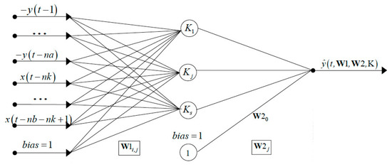
Figure 1.
IODNN with an ARX regressor [45].
After an initial selection of the number of hidden neurons (s), the input matrix, and the transfer function (K), the training is performed by solving a least squares non-linear optimization problem using the Levenberg–Marquardt approximation [46] and the adaptive search direction [44]. The core of the modeling problem concerning the ANN construction is that, normally, the user has to select the dimension of the model’s input and its components; therefore, in this application the selection of both the model’s input and the number of hidden neurons for IODNN is a combinatorial problem because, for a given accuracy, there is a great number of possible combinations to examine in order to look for the optimal solution in terms of the coefficient of determination (CoD). Finally, all possible results are selected by minimizing three objective functions: the number of input variables, the number of hidden neurons, and (1 − CoD).
2.2. Evolutionary Polynomial Regression (EPR)
ANNs models, even if able to describe complex phenomenon learning from data, do not permit the return of an explicit formula and do not provide a clear relationship between input parameters and output. An alternative is represented by EPR techniques [45] that use an evolutionary search to determine the structure of the polynomial expression and the least squares approach to determine the regression coefficient.
The EPR technique is a two-stage technique for constructing symbolic models: structure identification and parameter estimation. The EPR searches for symbolic polynomial structures in the first stage using a simple genetic algorithm (GA) and estimates constant values of polynomials by solving a least squares (LS) linear problem in the second stage, thus assuming a biunique relationship between a structure and its parameters [37].
The EPR framework allows the user to choose among different pseudo-polynomial expression structures:
where aj = adjustable parameter for the jth term; = optional bias; m = number of terms in the polynomial expression; Xk = the kth column of the matrix of inputs X; ES = matrix of candidate exponents; f(•) is a function defined by the user among a set of available functions (logarithm, exponential, hyperbolic tangent, hyperbolic secant); and Y = vector of outputs.
The search process performed by EPR within the domain of solution starts from the model structure (Equation (6)) chosen by the user. EPR looks for the best form of the function, thanks to the GA search paradigm, and performs the parameter estimation of aj by means of the singular value decomposition (SVD) in order to make the process of finding the solution to the LS problem more robust.
In order to avoid overfitting of returned models to training data, EPR tries to exploit the known principle of parsimony by finding the optimal compromise between the model simplicity and the accuracy of the regression-based returned model. EPR can achieve this purpose by penalizing the complexity of the returned expressions, controlling the variance of coefficients aj with respect to their values, and, finally, controlling the variance of polynomial terms with respect to the variance of residuals. Once this procedure has been completed, the user obtains a set of optimal model solutions of increasing complexity and different accuracy according to the above-described reasoning. In order to fully exploit the abilities of the EPR, the set of candidate exponents needed to build the matrix ES has to include the exponent 0 among others. This allows the search procedure to include in the best formulas the most important inputs among those available.
Giustolisi and Savic [47] improved the original version of EPR with a multi-objective genetic algorithm (MOGA-EPR). This algorithm changes the number of m pseudo-polynomial terms maximizing the model accuracy, minimizing the number of polynomial coefficients, and, finally, minimizing the number of inputs. The search into the space of solutions problem is solved using a MOGA approach based on the Pareto dominance criterion, which is named OPTIMOGA. This algorithm makes the EPR search faster because the search for all models (j = 1, 2, …, m) is performed simultaneously. Therefore, in the evaluation of the more complex optimal expressions, the presence of such inputs becomes a key point for the final choice of the best model.
3. Case Study
Starting from the state of the art and the literature data, ANNs and EPR models have been applied for predicting PATs performances. ANNs and EPR are both nonlinear global stepwise regression approaches providing a sensitivity analysis and a symbolic formulation, respectively, of the relation between inputs and output datasets. The analysis has been supported by an input literature database [6,13,16,30,31,33,38,39,40] including 33 pumps operating with a wide range of specific speeds and impeller sizes. The aim of this study has been to forecast BEP performance of a PAT starting from the operative data referred to BEP of a pump in direct mode. The input values for model training are represented using flow rate (QBEPp), water head (HBEPp), efficiency (ηBEPp), and specific speed (Nsp) related to the BEP in direct mode; whereas output values for model training are represented using flow rate (QBEPt), water head (HBEPt), efficiency (ηBEPt), and specific speed (Nst) related to the BEP in turbine mode, as well as flow ratio (q) and head ratio (h). On the whole, an input dataset of 132 records and 198 output data points were adopted into the study.
4. Results and Discussion
4.1. ANNs Application
ANNs methodology does not furnish a formula or a well-defined relation to describe a physical process but permits one to evaluate the real weight of each input candidate parameter.
The optimization parameters used for all ANNs applications were respectively:
- a hyperbolic tangent transfer function for the neurons also named kernel function;
- an optimization strategy based on three objective functions to minimize: the number of hidden neurons, the number of inputs, and the value of the function 1 − CoD for fitness on the validation set;
- a number of generations equal to 100;
- a maximum initial number of hidden neurons equal to 12;
- first layer bias and second layer bias used as decision variables;
- a maximum number of estimated parameters equal to 73.
Results of every ANN prediction are summarized into a table where W10 and W20 are the first and the second-layer bias indicators, # Xi is the dimension of the model input, # Hid is the number of the hidden neurons, # W is the number of weights, and % W is the percentage of the weights considering the maximum number as a reference.
4.1.1. ANNs Prediction for Nst
The ANNs methodology found a Pareto front size of 11 solutions for the specific speed number Nst. Full details of results are reported in Table 2. Results revealed that the IONN model characterized by the maximum number of inputs and hidden neurons was also characterized by the higher CoD value; however, models more parsimonious in terms of hidden neurons and inputs exhibit optimal performances and the difference between the first and the remaining was irrelevant. Moreover, solutions were characterized by an 88% average reduction in total parameters and the total inputs were selected only twice.
Table 2.
Pareto front (min(neurons, inputs, 1 − CoD)) of IONNs for Nst.
For the sake of clarity, the sensitivity analysis revealed a preeminent role of Nsp that appeared in all models, followed by the water head HBEPt and efficiency ηBEPt. These data confirm the decisive role that Nsp exercising on Nst, also confirmed by literature [30,32,33], and starting from this consideration, the best model, indicated with a gray line (Model 8), has been selected by taking into account both its parsimony in terms of parameters and its prediction performance.
4.1.2. ANNs Prediction for QBEPt
The ANNs methodology found a Pareto front size of nine solutions for the flow rate QBEPt (Table 3). Results reveal again that the IONN model characterized by the maximum number of inputs and hidden neurons was also characterized by the higher CoD value and the solutions were characterized by an 89% average reduction in total parameters and the complete set of inputs was selected only once.
Table 3.
Pareto front (min(neurons, inputs, 1 − CoD)) of IONNs for QBEPt.
Results revealed an irrefutable role of QBEPp that appeared in all models, followed by the efficiency ηBEPp. On the whole, models having QBEPp and ηBEPp as input variables revealed higher performance in terms of parsimony.
The best model, indicated with a gray line (Model 7), even if not characterized by the higher performance, was selected by taking into account both its parsimony in terms of parameters and its prediction performance.
4.1.3. ANNs Prediction for HBEPt
The ANNs methodology found a Pareto front size of eight solutions for the head rate HBEPt (Table 4). Results highlighted again that the IONN model characterized by the maximum number of inputs and hidden neurons was also characterized by the higher CoD value.
Table 4.
Pareto front (min(neurons, inputs, 1 − CoD)) of IONNs for HBEPt.
Also, solutions in this case were characterized by an 89% average reduction in terms of candidate inputs and hidden neurons. The total inputs were selected only twice. Results demonstrate an irrefutable role of HBEPp, which was present in all models, followed by the specific speed Nsp and efficiency ηBEPp. The best model, indicated with a gray line (Model 7), was selected by taking into account both its parsimony in terms of parameters and its prediction performance, also confirmed by the technical literature [30,33].
4.1.4. ANNs Prediction for ηBEPt
The ANNs methodology found a Pareto front size of only three solutions for the efficiency ηBEPt (Table 5), even if these solutions were all characterized by a CoD of about 0.83. Paying attention to the results, it was very interesting to verify that ηBEPt depends on the pump efficiency ηBEPp.
Table 5.
Pareto front (min(neurons, inputs, 1 − CoD)) of IONNs for ηBEPt.
Solutions were characterized by an 91% average reduction in total parameters. The best model, indicated with a gray line (Model 2), as selected by taking into account both its parsimony in terms of parameters and its prediction performance.
4.1.5. ANNs Prediction for q and h
A separate discussion must be made for the results of the analysis conducted for the flow ratio q and head ratio h. The ANNs methodology found, respectively, a Pareto front size of only four solutions for the q (Table 6) and two for h (Table 7), which, except one for q, were all characterized by a very low coefficient of determination. This situation was dramatic for h, highlighting how input data did not permit a fit for the returned models. Starting from this result, an attempt was made by changing the transfer function from hyperbolic tangent to linear. This attempt gave slightly better results for h but worse for q, and the obtained results are summarized into Table 8 and Table 9, respectively.
Table 6.
Pareto front of IONNs for q for a hyperbolic tangent transfer function.
Table 7.
Pareto front of IONNs for h for a hyperbolic tangent transfer function.
Table 8.
Pareto front of IONNs for q for a linear transfer function.
Table 9.
Pareto front of IONNs for h for a linear transfer function.
However, as verified in Reference [35], the obtained results for q and h did not satisfy in terms of prediction and accuracy.
4.2. EPR Application
With the aim to discover a relationship between the specific speed number Nst, the flow ratio q, and the head ratio h, the candidate input data set the model structure adopted in this study as the following:
The exponents ranging from −3 to 3 with a step of 0.5 were selected to limit the dimension of the search space, and consequently, the complexity of the identified models. The models’ size m was fixed to four terms (flow rate QBEPp, water head HBEPp, efficiency ηBEPp at the BEP, and specific speed Nsp). Moreover, a bias was selected into the program and LS parameter estimation was constrained to search for the set of positive polynomial coefficient values aj.
The MOGA optimization model adopted into the study focused its attention on the optimization problem of three objective functions: the minimization of the number of input Xi, the minimization of the number of terms m, and, finally, the maximization of model accuracy. The EPR-MOGA conducts a number of generations, that in this case was 1080, a number that depended on the number of candidate inputs, length of training set, exponents, and maximum number of monomial terms of each model.
The fitness of every prediction model was based on the evaluation of coefficient of determination (CoD), and EPR-MOGA returned a number of models thanks to a Pareto set that returned the best compromise between the model parsimony and the experimental data fitting. In the following tables, only the best models of every analyzed output and the relative CoD, number of input candidates, and number of polynomial coefficients are summarized.
4.2.1. EPR Prediction for Nst
EPR identified 15 non-dominated models for Nst with varying structural complexity and performance, ranging from a linear model (Equation (8)) to more complex models (Equations (11) and (12)). Table 10 reports the main characteristics of these formulas, and it can be observed how more complex models do not return a significant CoD increase, even when Equation (8) is characterized by a very high CoD. Comparing the selected formulas, one can observe that all contain the specific speed velocity Nsp; however, Equation (8) is very close to the experimental ones found by Yang et al. [31] and Stefanizzi et al. [33]. Figure 2 compares literature data versus Equation (8) models [31,33].
Table 10.
Models returned by EPR-MOGA for Nst.
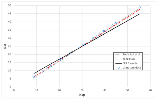
Figure 2.
PAT-specific speed versus pump-specific speed.
4.2.2. EPR Prediction for QBEPt
EPR returned 11 models for QBEPt, where the first three are simple formulas, while the others are complex models and also difficult to explain from a physical point of view. For these reasons, Table 11 summarized the first three and one of the remaining ones. However, by analyzing the obtained models, Equation (13) has been chosen for its physical meaning; Figure 3 compares literature data with that obtained by the selected formula.
Table 11.
Models returned by EPR-MOGA for QBEPt.
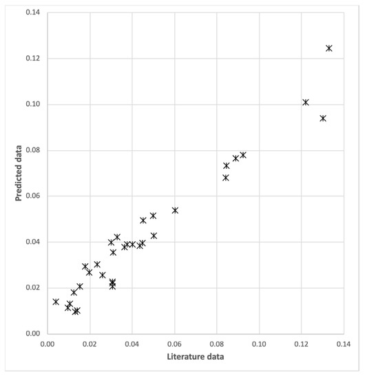
Figure 3.
Predicted data versus literature data.
4.2.3. EPR Prediction for HBEPt
EPR returned eight models for HBEPt, where the first three are simple formulas while others are complex models and also difficult to explain from a physical point of view. For these reasons, Table 12 summarizes the first three, and for the sake of example only, one of the remaining. However, analyzing the obtained models, Equation (18) has been chosen for its physical meaning; the selected model is also quite close to what is reported by the technical literature [18,19,20,21].
Table 12.
Models returned by EPR-MOGA for HBEPt.
4.2.4. EPR Prediction for ηBEPt
EPR returned eight models for ηBEPt. In this case, also, the first formulas, except the first one characterized by a very low CoD, are rather simple while the remaining are complicated. For these reasons, Table 13 summarized the more interesting obtained models, it Equation (22) was selected both for its simplicity and for its good compromise between parsimony and data fitting.
Table 13.
Models returned by EPR-MOGA for ηBEPt.
4.2.5. EPR Prediction for q and h
Unlike what was found for other parameters and as already happened for the ANN predictions, the application of EPR to q and h did not provide useful results.
EPR identified 11 non-dominated models for q with varying structural complexity and performance; however, it can be seen that there was a very low CoD for each of the identified models. Table 14 reports the main characteristics of these formulas. Meanwhile, EPR identified only five models for h and Table 15 reports the main characteristics of these model.
Table 14.
Models returned by EPR-MOGA for q.
Table 15.
Models returned by EPR-MOGA for h.
The retrieved models do not furnish CoD with interesting values despite Equation (27) for the first case and Equation (30) for the latter being quite similar to those retrieved thanks to literature test rigs [19,20,21].
5. Conclusions
The paper conducted a sensitivity analysis on the input parameters that most influence a pump performance in reverse mode and offers a comparison between ANNs and EPR methodologies in order to increase knowledge about different models for the prediction of PAT behavior. Literature data summarized several studies based on experimental tests or numerical application, and overall, these methods can be subdivided into a first category based on the best efficiency point (BEP) parameters and a second one based on the specific speed number Nsp. Starting from this knowledge, the paper provides a numerical analysis with the aim to understand the real weight of every input parameter on the output ones.
The ANN approach, while containing the intrinsic limit of not providing a well-defined formula, gives the user the possibility to identify the structure of the best model, emphasizing the correlation among the most influential input factors and the output [45]. The EPR technique, instead, is able to provide a clear formula, but in this study, this research was not simple and understandable in all cases. The use of one methodology did not exclude the other because while ANN needs a preliminary selection of the transfer function, the latter does not need an a priori knowledge of the model structure.
Overall, the paper, thanks to the application of ANNs, highlighted the real weight of each input parameter on the outputs, and this is certainly an advantage and benefit to the scientific research on this topic in the near future. Whereas, EPR application returned general formulas with a high coefficient of determination values, the selected formulas for every output parameter had values of CoD of about 0.75, except for the specific speed Nst, where the value was equal to 0.95.
Both methods were not able to relate the flow ratio q and head ratio h to the input candidate variables, in agreement with Reference [35], and this should mean that it is probably necessary to deepen this aspect with wider experimental tests.
The results of this sensitivity analysis point out that while parameters like Nst certainly depend on well-defined input parameters, others like q and h instead show a low correlation with the input parameters, and for this reason, they are probably not able to provide a general formula for predicting the pump performance in a reverse mode, knowing those of a pump in a direct mode. As a whole, the study showed how the application of two different methodologies from a mathematical point of view leads to absolutely consistent results.
In conclusion, the results of this study may represent a starting point for future research, thanks to experimental apparatus and numerical approaches, that will be able to make use of this sensitivity analysis and to focus its efforts on the most influencing input parameters, such as the specific speed Nst, on the evaluation of PAT performances.
Funding
This research received no external funding.
Conflicts of Interest
The author declares no conflict of interest.
Nomenclature
List of general symbols and indexes used in the paper.
| Q | (m3/s) | flow rate |
| H | (m) | water head |
| q | (-) | flow ratio |
| h | (-) | head ratio |
| η | (-) | efficiency |
| n | (rpm) | rotational speed |
| Ns | (-) | specific speed number (Q in (m3/s), H in (m) and n in (rpm)) |
| D | (m) | impeller diameter |
| P | (W) | power |
| (kg/m3) | fluid density | |
| (m/s2) | gravitational constant | |
| (-) | flow number | |
| (-) | head number | |
| (-) | power number | |
| Ng | (rpm) | generator rotational speed |
| Nm | (rpm) | mechanical rotational speed |
| ω | (rad/s) | rotational speed |
| D0 | (m) | impeller diameter at the outlet position |
| Ds | (-) | impeller specific diameter defined as |
| ηhp | (-) | hydraulic efficiency defined as |
| f | (Hz) | frequency |
| p | (-) | number of poles |
| aj, a0 | (-) | jth polynomial coefficient in the EPR model |
| CoD | (-) | coefficient of determination |
| ES | (-) | matrix of exponents of input variables in the EPR model |
| f | (-) | functions that can be selected in the EPR model structure |
| LS | (-) | least squares |
| m | (-) | number of polynomial terms in the EPR model |
| SSE | (-) | sum of squared errors |
| Xi | (-) | ith EPR input variable |
| Y | (-) | vector of target values |
| ŷ(t, W1, W2, K) | (-) | model’s output |
| φ(t) | (-) | input at time t |
| W1, W2 | (-) | first and second layer weights |
| Kj | (-) | kernel function |
| W1i,j | (-) | weights in ANNS |
| nb | (-) | number of inputs x |
| na | (-) | number of outputs y |
| nk | (s) | related delay expressed |
| K | (-) | transfer function |
| s | (-) | hidden neurons number |
| p | pump mode | |
| t | turbine mode | |
References
- European Environmental Agency. Electric Vehicles in Europe. 2016. Available online: https://www.eea.europa.eu/publications/electric-vehicles-in-europe (accessed on 5 October 2018).
- Jain, S.V.; Patel, R.N. Investigations on pump running in turbine mode: A review of the state-of-the-art. Renew. Sustain. Energy Rev. 2014, 30, 841–868. [Google Scholar] [CrossRef]
- World Energy Council. World Energy Resources 2016. 2016. Available online: https://www.worldenergy.org/wp-content/uploads/2017/03/WEResources_Hydropower_2016.pdf (accessed on 5 October 2018).
- Meirelles Lima, G.; Luvizotto, E.; Brentan, B.M. Selection and location of Pumps as Turbines substituting pressure reducing valves. Renew. Energy 2017, 109, 392–405. [Google Scholar] [CrossRef]
- Muhammetoglu, A.; Karadirek, I.E.; Ozen, O.; Muhammetoglu, H. Full-Scale PAT Application for Energy Production and Pressure Reduction in a Water Distribution Network. J. Water Resour. Plan. Manag. 2017, 143, 8. [Google Scholar] [CrossRef]
- Rossi, M.; Righetti, M.; Renzi, M. Pump-as-turbine for Energy Recovery Applications: The Case Study of An Aqueduct. Energy Procedia 2016, 101, 1207–1214. [Google Scholar] [CrossRef]
- Puleo, V.; Fontanazza, C.M.; Notaro, V.; De Marchis, M.; Gabriele Freni, G.; La Loggia, G. Pumps as turbines (PATs) in water distribution networks affected by intermittent service. J. Hydroinform. 2014, 16, 259–271. [Google Scholar] [CrossRef]
- Samora, I.; Manso, P.; Franca, M.J.; Schleiss, A.J.; Ramos, H.M. Energy recovery using micro-hydropower technology in water supply systems: The case study of the city of Fribourg. Water 2016, 8, 344. [Google Scholar] [CrossRef]
- Balacco, G.; Binetti, M.; Caporaletti, V.; Gioia, A.; Leandro, L.; Iacobellis, V.; Sanvito, C.; Piccinni, A.F. Innovative mini-hydro device for the recharge of electric vehicles in urban areas. Int. J. Energy Environ. Eng. 2018, 9, 435–445. [Google Scholar] [CrossRef]
- Binama, M.; Su, W.T.; Li, X.B.; Li, F.C.; Wei, X.Z.; Shi, A. Investigation on pump as turbine (PAT) technical aspects for micro hydropower schemes: A state-of-the-art review. Renew. Sustain. Energy Rev. 2017, 79, 148–179. [Google Scholar] [CrossRef]
- Carravetta, A.; Fecarotta, O.; Del Giudice, G.; Ramos, H. Energy Recovery in Water Systems by PATs: A Comparisons among the Different Installation Schemes. Procedia Eng. 2014, 70, 275–284. [Google Scholar] [CrossRef]
- Chapallaz, J.M.; Eichenberger, P.; Fischer, G. Manual on Pumps Used as Turbines; MHPG Series: Eschborn, Germany, 1992; ISBN 3-528-02069-5. [Google Scholar]
- Singh, P. Optimization of Internal Hydraulics and of System Design for Pumps as Turbines with Field Implementation and Evaluation. Ph.D. Thesis, University of Karlsruhe, Karlsruhe, Germany, 2005. [Google Scholar]
- Bozorgi, A.; Javidpour, E.; Riasi, A.; Nourbakhsh, A. Numerical and experimental study of using axial pump as turbine in Pico hydropower plants. Renew. Energy 2013, 53, 258–264. [Google Scholar] [CrossRef]
- Jain, S.; Swarnkar, A.; Motwani, K.; Patel, R. Effects of impeller diameter and rotational speed on performance of pump running in turbine mode. Energy Convers. Manag. 2015, 89, 808–824. [Google Scholar] [CrossRef]
- Rossi, M.; Renzi, M.A. Analytical Prediction Models for Evaluating Pumps-As-Turbines (PaTs) Performance. Energy Procedia 2017, 118, 238–242. [Google Scholar] [CrossRef]
- Fontana, N.; Giugni, M.; Glielmo, L.; Marini, G.; Zollo, R. Hydraulic and Electric Regulation of a Prototype for Real-Time Control of Pressure and Hydropower Generation in a Water Distribution Network. J. Water Resour. Plan. Manag. 2018, 144, 11. [Google Scholar] [CrossRef]
- Stepanoff, A.J. Centrifugal and Axial Flow Pumps: Theory, Design and Application; John Wiley: New York, NY, USA, 1957. [Google Scholar]
- Childs, S.M. Convert pumps to turbines and recover HP. Hydro Carbon Process. Pet. Refin. 1962, 41, 173–174. [Google Scholar]
- Hancock, J.W. Centrifugal pump or water turbine. Pipe Line News, 1963; 25–27. [Google Scholar]
- McClaskey, B.M.; Lundquist, J.A. Can You Justify Hydraulic Turbines? Hydrocarb. Process. 1976, 55, 163–169. [Google Scholar]
- Sharma, K. Small Hydroelectric Project-Use of Centrifugal Pumps as Turbines; Technical Report; Kirloskar Electric Co.: Bangalore, India, 1985. [Google Scholar]
- Gopalakrishnan, S. Power recovery turbines for the process industry. In Proceedings of the Third International Pump Symposium, Houston, TX, USA, 20–22 May 1986; Texas A&M University: College Station, TX, USA, 1986; pp. 3–11. [Google Scholar]
- Schmiedl, E. Serien-Kreiselpumpen im Turbinenbetrieb; Pumpentagung: Karlsruhe, Germany, October 1988. [Google Scholar]
- Alatorre-Frenk, C. Cost Minimization in Micro Hydro Systems Using Pumps-as-Turbines. Ph.D. Thesis, University of Warwick, Coventry, UK, 1994. [Google Scholar]
- Sharma, R.L. Pumps as turbines (PAT) for small hydro. In Proceedings of the International Conference on Hydro Power Development in Himalayas, Shimla, India, 20–22 April 1998; pp. 137–146. [Google Scholar]
- Nautiyal, H.; Varun, K.A.; Yadav, S. Experimental investigation of centrifugal pump working as turbine for small hydropower systems. Energy Sci. Technol. 2011, 1, 79–86. [Google Scholar]
- Grover, K.M. Conversion of Pumps to Turbines; GSA InterCorp.: Katonah, NY, USA, 1980. [Google Scholar]
- Lewinsky-Keslitz, H.P. Pumpen als Turbinen fur Kleinkraftwerke. Wasser-Wirtschaft 1987, 77, 531–537. [Google Scholar]
- Derakhshan, S.; Nourbakhsh, A. Experimental study of characteristic curves of centrifugal pumps working as turbines in different specific speeds. Exp. Therm. Fluid Sci. 2008, 32, 800–8077. [Google Scholar] [CrossRef]
- Yang, S.S.; Derakhshan, S.; Kong, F.Y. Theoretical, numerical and experimental prediction of pump as turbine performance. Renew. Energy 2012, 48, 507–513. [Google Scholar] [CrossRef]
- Tan, X.; Engeda, A. Performance of centrifugal pumps running in reverse as turbine: Part II—Systematic specific speed and specific diameter based performance prediction. Renew. Energy 2016, 99, 188–197. [Google Scholar] [CrossRef]
- Stefanizzi, M.; Torresi, M.; Fortunato, B.; Camporeale, S.M. Experimental investigation and performance prediction modeling of a single stage centrifugal pump operating as turbine. Energy Procedia 2017, 126, 589–596. [Google Scholar] [CrossRef]
- Venturini, M.; Alvisi, S.; Simani, S.; Manservigi, L. Comparison of Different Approaches to Predict the Performance of Pumps as Turbines (PATs). Energies 2018, 11, 1016. [Google Scholar] [CrossRef]
- Rossi, M.; Renzi, M. A general methodology for performance prediction of pumps-as-turbines using Artificial Neural Networks. Renew. Energy 2018, 128, 265–274. [Google Scholar] [CrossRef]
- Giustolisi, O.; Simeone, V. Multi-Objective Strategy in Artificial Neural Network Construction. Hydrol. Sci. J. 2006, 3, 502–523. [Google Scholar] [CrossRef]
- Giustolisi, O.; Kapelan, Z.; Savic, D.A. Multi-objective Evolutionary Polynomial Regression. In Proceedings of the 7th International Conference on Hydroinformatics (HIC 2006), Nice, France, 4–8 September 2006; Gourbesville, P., Cunge, J., Liong, V.G.S.Y., Eds.; Research Publishing, 2006; Volume 1, pp. 725–732. [Google Scholar]
- Barbarelli, S.; Amelio, M.; Florio, G. Experimental activity at test rig validating correlations to select pumps running as turbines in microhydro plants. Energy Convers. Manag. 2017, 107, 103–121. [Google Scholar] [CrossRef]
- Giosio, D.R.; Henderson, A.D.; Walker, J.M.; Brandner, P.A.; Sargison, J.E.; Gautam, P. Design and performance evaluation of a pump-as-turbine micro-hydro test facility with incorporated inlet flow control. Renew. Energy 2015, 78, 1–6. [Google Scholar] [CrossRef]
- Pugliese, F.; De Paola, F.; Fontana, N.; Giugni, M.; Marini, G. Experimental characterization of two Pumps as Turbines for hydropower generation. Renew. Energy 2016, 99, 180–187. [Google Scholar] [CrossRef]
- Haykin, S. Neural Networks: A Comprehensive Foundation, 2nd ed.; Prentice-Hall Inc.: Englewood Cliffs, NJ, USA, 1999. [Google Scholar]
- Ljung, L. System Identification: Theory for the User, 2nd ed.; Prentice-Hall Inc.: Upper Saddle River, NJ, USA, 1999. [Google Scholar]
- Giustolisi, O. Input-output dynamic neural networks simulating inflow-outflow phenomena in an urban hydrological basin. J. Hydroinform. 2000, 2, 269–279. [Google Scholar] [CrossRef]
- Giustolisi, O.; Laucelli, D. Improving generalization of artificial neural networks in rainfall-runoff modeling. Hydrol. Sci. J. 2005, 50, 439–457. [Google Scholar] [CrossRef]
- Laucelli, D.; Giustolisi, O.; Savic, D. 2009 Data-based modeling: A comparison between Artificial Neural Networks and Evolutionary Polynomial regression. In Proceedings of the Conference on Hydroinformatics (HIC 2009), Concepcion, Chile, 19–21 August 2009. [Google Scholar]
- Kisi, Ö. Multi-layer perceptrons with Levenberg-Marquardt training algorithm for suspended sediment concentration prediction estimation. Hydrol. Sci. J. 2004, 49, 1025–1040. [Google Scholar] [CrossRef]
- Giustolisi, O.; Savic, D. Advances in data-driven analyses and modelling using EPR-MOGA. J. Hydroinform. 2009, 11, 225–236. [Google Scholar] [CrossRef]


© 2018 by the author. Licensee MDPI, Basel, Switzerland. This article is an open access article distributed under the terms and conditions of the Creative Commons Attribution (CC BY) license (http://creativecommons.org/licenses/by/4.0/).