Abstract
To detect the categories and positions of various transformer components in inspection images automatically, this paper proposes a transformer component detection model with high detection accuracy, based on the structure of Faster R-CNN. In consideration of the significant difference in component sizes, double feature maps are used to adapt to the size change, by adjusting two weights dynamically according to the object size. Moreover, different from the detection of ordinary objects, there is abundant useful information contained in the relative positions between components. Thus, the relative position features are defined and introduced to the refinement of the detection results. Then, the training process and detection process are proposed specifically for the improved model. Finally, an experiment is given to compare the accuracy and efficiency of the improved model and the original Faster R-CNN, along with other object detection models. Results show that the improved model has an obvious advantage in accuracy, and the efficiency is significantly higher than that of manual detection, which suggests that the model is suitable for practical engineering applications.
1. Introduction
With the popularization of inspection robots and the accumulation of image data in smart substations, the automatic recognition of power equipment states based on inspection images is increasingly being widely used, such as switch state recognition and insulator breakage identification [1,2,3]. Compared with the traditional manual inspection, the computer vision technology can effectively improve the inspection frequency and efficiency, and avoid the influence of subjectivity on the accuracy [4,5]. As one of the most important parts in substations, the main transformers have a bearing on the safety and reliability of the power system. Thus, defect and fault recognition based on transformer images has important practical value, in which the detection of transformer components is an essential step. Only when the categories and positions of transformer components are detected accurately, can the recognition algorithm be designed for possible defects and faults of different components, such as oil leakage of conservators, silica gel discoloration of breathers and so on.
Traditional detection methods for power equipment and components are mainly rule-based algorithms with low-level features (e.g., Scale Invariant Feature Transform (SIFT) [6], Histograms of Oriented Gradient (HOG) [7]). Although these methods are intuitive and interpretable, they are hard to adapt to complex scenes and usually require abundant manual workloads for tuning when applied to a new scene [8]. In the computer vision field, the practice in recent years shows that the object detection models based on deep learning can abstract and synthesize the low-level features, which obtains substantially higher accuracy on PASCAL VOC and other canonical data sets [9,10,11,12,13]. However, when the deep learning detection models used in ordinary objects (e.g., cars, plants) are directly applied to transformer component detection, the accuracy is still unsatisfactory for defect and fault recognition. On the one hand, the difference between the sizes of various transformer components is considerably large, which will affect the accuracy significantly. On the other hand, unlike ordinary objects, there are relatively fixed relations between the positions of transformer components, while detection models for ordinary objects cannot make full use of the relative position information. Thus, focusing on these problems, this paper proposes an improved model based on Faster Region-based Convolutional Neural Network (Faster R-CNN) [11], which is a classical deep learning network with relatively high accuracy in object detection.
One of our improvements is to dynamically handle the sharp difference in component sizes in transformer inspection images. The problem of object size difference is studied in some research, in which multi-scale feature maps are commonly used to adjust to different object sizes [12,14]. In this paper, the idea of multi-scale feature maps is also adopted, but a weight is assigned to each feature map, which can change dynamically according to the object sizes in the detection process. To simplify the model structure, we select just two feature maps with different levels of features, and then design a calculation method to adjust the two weights of the two feature maps as the object sizes change. Based on the two weights, the predicted results of the two feature maps are combined into a total result output by the neural network.
The other improvement in this paper is the consideration of the relative position relations between different components. In the detection of ordinary objects, there is often no apparent relative position relation between the targets, but for transformer components, the relative position relations are fairly common and relatively fixed. In fact, when people recognize transformer components in inspection images with eyes, they often locate the components with the aid of their relative positions. For example, most people will firstly recognize the components with large sizes, and then search for small components around the large ones rather than by scanning the whole image. In other words, the components in an image are not detected at the same time but in an iterative way. Noticing this problem, we specifically propose a calculation method of relative position features, which are used to refine the predictions iteratively in the detection process. Meanwhile, in the iterations, the order of components detected has uncertainties, and the components that have not been detected or do not exist (e.g., obscured by other things) in an image will lead to missing values in relative position features. Thus, we adopt random forests models for refinement, which are robust to missing values, and we design the models in detail, according to the characteristics of the relative position features.
In our experiments, the improved Faster R-CNN is compared with several state-of-the-art object detection models, including the original Faster R-CNN [11]. Additionally, aiming at our two improvements, we employ two models as controls to directly present the advantage of each improvement. The results show that the improved Faster R-CNN has an obvious increase in accuracy, which can satisfy the requirements for defect and fault recognition.
2. Related Work
In the power industry, to realize the automatic detection of power equipment and components, several object detection methods have been proposed in intuitive ways. Based on the matching of templates, the authors of [15,16] manually framed an object in an existing image as a template, and applied it to match corresponding objects in new images. This method is sensitive to the precision of the camera location and angle, so the accuracy and stability is difficult to guarantee [8]. To improve the robustness to the camera location and angle, some researchers artificially constructed some features according to the shapes and outlines of the objects, and then detected the objects by analyzing the features extracted from images. For example, the authors of [17,18,19,20] constructed the features related to geometric figures (i.e., straight lines and circles) for buses, transmission lines and insulators, and extracted the features based on Hough transform and curvature scale space for object detection. These methods have better stability, but are only suitable for components with simple shapes and need to artificially construct features for each type of components. Noticing these problems, some researchers adopted machine learning algorithms to reduce the requirement of feature construction and enhance the generalization ability of models. For example, the authors of [8] just extracted the basic features related to gradients and colors of images without special construction towards objects, and sent the features to Hough forests to detect substation switches. Although the features adopted in the research above, whether artificially constructed or not, are limited to a low level without hierarchical and multi-stage processes [9], they prove to us that the consideration of the characteristics of power equipment and components is beneficial to improving the effect of feature extraction.
In the computer vision field, after deep learning was introduced into object detection [9,21], deep networks rapidly became the mainstream models because of their advantages in accuracy. In recent years, abundant research has been carried out to further improve the performance of deep learning models, among which some ideas are somewhat similar to our two improvements.
To deal with the difference between object sizes, the authors of [22,23] combined multiple levels of feature maps together with techniques of region of interest (RoI) pooling, deconvolution, etc., and then detected various sizes of objects based on the integrated feature map. Further, the authors of [12,14,24] directly carried out predictions on each extracted feature map instead of integrating them, which is more effective to adapt to the size change of objects. Recently, the authors of [25] also adopted multi-scale feature maps based on the classical one-stage model YOLO [26], and improved the accuracy mainly on small object detection. Although multiple feature maps are beneficial to the adaptation to the size difference, they consume more time in the detection process, which is an obvious problem especially for two-stage models like Faster R-CNN. Moreover, to obtain higher efficiency, the authors of [27] designed scale-transfer layers to obtain high-resolution feature maps with few additional parameters and computational overhead. In this paper, we also predict results on multiple extracted feature maps. Additionally, we assign different weights that dynamically vary with object sizes to different levels of feature maps, inspired by the idea that low-level feature maps with high resolutions perform better in detecting small objects while the high-level feature maps are more suitable for large ones [23].
Our second improvement is based on the idea that people detect multiple objects in an iterative way, which is also noticed in some other research. The authors of [28] analyzed the statistical relation between the sample distribution and the intersection over union (IoU) threshold, and designed a cascade network in which the objects are detected in several stages using different IoU thresholds; the authors of [29] observed the statistics of failure cases of some detection models and argued that false positives affect the accuracy significantly, and thus proposed a decoupled classification refinement (DCR) network to further refine the classification results of Faster R-CNN. However, statistical results vary from one data set to another, and may even change in the iterative process. Thus, the accuracy will decrease instead of increase, particularly when the number of iterations exceeds a certain value [30]. In terms of this problem, the authors of [30] specifically proposed an optimization-based refinement method, in order to keep the accuracy rising in the iterative process. On the other hand, similar to our concerns, some research tried to design a network that detects objects in a way more similar to the visual process of human beings. In consideration of the domain adaptive ability of human eyes, the authors of [31] added two branches to Faster R-CNN on the image level and instance level, and adopted adversarial training and consistency regularization to enhance domain invariance of the network. In addition, the authors of [32] mimicked the population Receptive Field (pRF) and introduced dilated convolution layers into Inception block [33] to improve the feature extraction effect.
3. Improved Faster R-CNN for Transformer Component Detection
3.1. Architecture of Improved Faster R-CNN
According to the introduction of [11], the architecture of Faster R-CNN is expressed as Figure 1, which can be divided into three modules: feature extraction, proposal (a box that may contain an object) generation, and category and position detection. Considering the requirement of accuracy and the scale of the data set in this paper, the ResNet-50 is selected as the convolutional neural network (i.e., Stage 1–Stage 5) in the feature extraction module [34]. As shown in Figure 1, an image is transformed into a feature map by 5-stage ResNet-50 firstly, and then the feature map is sent to a region proposal network (RPN) to generate n proposals, each of which has 2 probabilities of containing an object or not containing an object, and 4 coordinates encoding the proposal position. Finally, the feature map and n1 selected proposals are sent to region of interest (RoI) pooling, fully-connected (FC) layers and a softmax classifier/bounding-box regressor. After that, each of the n1 proposals has k + 1 probabilities of containing k categories of objects plus a “background” category, and 4k coordinates encoding k adjusted proposal positions of k object categories.
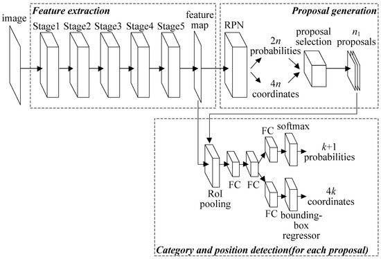
Figure 1.
Faster Region-based Convolutional Neural Network (Faster R-CNN) architecture.
Based on Faster R-CNN, the improved model is proposed as shown in Figure 2. Compared with Figure 1, there are two main improvements of the architecture in Figure 2. The first one is to add the feature map of Stage 2 to the category and position detection module, which cooperates with the feature map of Stage 5 to adapt to the change of component sizes dynamically. The second one is to introduce relative position features between components to both the proposal generation module and the category and position detection module, and adopt random forests (RF) models to refine the probabilities and coordinates.
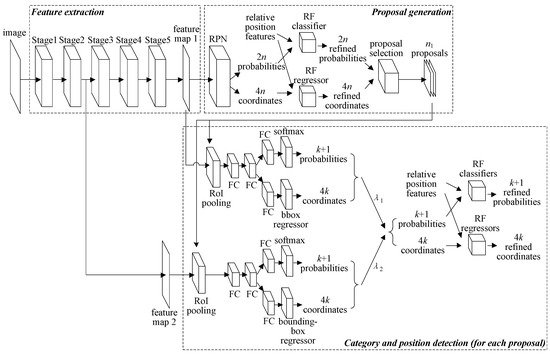
Figure 2.
Improved Faster R-CNN architecture.
3.2. Double Feature Maps for Different Component Sizes
In the category and position detection module, double feature maps generated by different stages of ResNet-50 are used for different component sizes. The feature level of feature map 1 is higher, which is beneficial to the feature abstraction of large objects, but it will lead to too much information loss for small objects in the process of convolution [22,23]. On the contrary, feature map 2 has a higher resolution and less information loss, but the feature level is relatively low and the features may not be abstract enough for large objects. To adjust to different object sizes dynamically, for each proposal, two groups of probabilities and coordinates are firstly generated based on the two feature maps separately, and then are weighted according to the proposal size. The calculation method of weight λ1 and λ2 is:
where sizepro represents the size of the proposal, and sizeave represents the average size of all the ground-truth boxes (a ground-truth box frames an object correctly) in the training set. According to Equations (1) and (2), the weights change linearly when sizepro < sizeave. Additionally, if the value of λ1 (λ2) is λ when sizepro = sizeave/t (t > 1), then the value of λ2 (λ1) is equal to λ when sizepro = t·sizeave. Once the weights λ1 and λ2 are obtained, each of the probabilities (coordinates) is calculated by two corresponding probabilities (coordinates) as:
where p1 and p2 represent two probabilities (coordinates) generated based on feature map 1 and feature map 2 respectively, and p represents a weighted probability (coordinate) of p1 and p2.
3.3. Relative Position Features of Components
In the proposal generation module and the category and position detection module, the relative position features between a proposal and the detected components are used to refine the probabilities and coordinates of the proposal. Assume that there are k categories of components in the detection task, and then there are at most k groups of relative position features for each proposal.
Let the position of a proposal be represented by four parameters: x, y, w and h, which denote the proposal’s center coordinates and its width and height. Likewise, let the ground-truth box of a detected component be represented by x*, y*, w* and h*, and the four position features of the proposal relative to the detected component are defined as:
where the denominators w* and h* are used to avoid the influence of the distance between the component and the camera, since they will change dynamically along with the distance. Thus, the relative position feature vector of each proposal has 4k dimensions representing the position features relative to k categories of components. If a component category has not been detected or does not exist in an image, the four feature values corresponding to the category are missing.
3.4. Random Forests for Refining Probabilities and Coordinates
After extracting the relative position feature vectors, we need to select a machine learning algorithm to refine the probabilities and coordinates. Because usually only parts of the components are detected during the refinements, the relative position feature vectors always contain missing values. The machine learning algorithms based on “distance measurement” of samples, such as k-nearest neighbors (k-NN), support vector machine (SVM) and logistic regression, are sensitive to missing values, and the accuracy is likely to decrease if the missing values are filled manually. Conversely, the decision tree algorithm and naive Bayes algorithm are robust to missing values and do not need manual filling. However, there are relatively strong correlations between the relative position features, which will affect the accuracy of the naive Bayes algorithm [35], so the random forests (RF) model based on the decision tree algorithm is selected for the refinement.
Consider the case in Figure 3, in which there are four training samples and two categories of components (i.e., k = 2), and Category 1 is not contained in Sample 1 while Category 2 is not contained in Sample 4. Intuitively speaking, “distance measurement” based algorithms consider one sample’s feature values (i.e., a row of feature values) at a time, while a decision tree evaluates one feature’s values (i.e., a column of feature values) at a time. If a feature value is missing in a sample’s row, the sample’s location in the feature space cannot be figured out, so all the feature values in the row will be unavailable; on the contrary, if a feature value is missing in a feature’s column, the feature only loses one value for evaluation, while the other values in the column are still available to evaluate the feature effectively [36]. More analyses in depth are as follows:
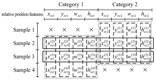
Figure 3.
A simple case of missing values. A symbol “×” represents a missing value in the corresponding feature.
For algorithms based on “distance measurement”, take logistic regression for example, of which the key issue is to minimize the loss function as:
where a is the number of available training samples, yi and xi are the label and the feature vector of the ith available training sample respectively, θ is a parameter vectors to be fitted, and hθ(x) is the logistic function. Because Sample 1 and Sample 4 contain missing values in the feature vector x, they cannot participate in the calculation of the loss function, and the available feature values are only the ones of Sample 2 and Sample 3 in the boxes with solid lines in Figure 3.
In contrast, the key issue of decision tree construction is to select one feature at a tree node to divide the samples and split out new nodes. Thus, each feature is examined in turn separately according to a splitting criterion. Take the feature xre1 for example, whose division points are chosen through bi-partition [37]. Without loss of generality, consider a division point x*re1 (i.e., if a sample’s xre1 value is less than x*re1, the sample will be assigned to the left child node, or else it will be assigned to the right child node) and choose Gini index [36] as the splitting criterion, then the index used in examining the division point x*re1 is calculated as:
where a is the total number of available training samples, a1 and a2 are the numbers of available training samples assigned to the left and right child nodes respectively, L1 and L2 are the sets of labels of available training samples assigned to the left and right child nodes respectively, and Gini(L) is the Gini index of the label set L. For the feature xre1, there are three available training samples (i.e., a = 3): Sample 2, Sample 3 and Sample 4, and thus are available feature values. In addition, the unavailable sample (i.e., Sample 1) can be assigned to the left or right child node using techniques like surrogate splits [36]. Similarly, the other features can be examined in the same way, so the available feature values are the ones in the boxes with dashed lines in Figure 3, with no feature values wasted.
Although examining each feature separately is effective in dealing with missing values, it will also lead to a problem that the samples need to be divided too many times when the division boundary is complex. To solve this problem, we establish multivariate decision trees inspired by [38]. At each tree node, instead of using one feature to divide the samples, we use four features of the same category (e.g., xre1, yre1, wre1 and hre1) at the same time and adopt their linear combination (denoted as l(xre1, yre1, wre1, hre1) for xre1, yre1, wre1 and hre1, which can be specifically calculated with techniques like least square method [38]) for division. Similar to Equation (9), denote a division point of l(xre1, yre1, wre1, hre1) as l*(xre1, yre1, wre1, hre1), then the index used in examining the division point is calculated as:
where a, a1, a2, L1, L2 and Gini(L) are the same meanings as those of Equation (9), but the training samples are assigned to the left or right child node according to l*(xre1, yre1, wre1, hre1) instead of x*re1. For the four features xre1, yre1, wre1 and hre1, there are still three available training samples (i.e., a = 3): Sample 2, Sample 3 and Sample 4. Similarly, the four features of Category 2 can be examined in the same way, so the available feature values are the ones in the boxes with dotted lines in Figure 3, with no feature values wasted.
Hypothetically, consider the case in Figure 4. For a univariate decision tree, according to the illustration above, the available feature values are the ones in the boxes with dashed lines. For our multivariate decision tree, because Sample 2 contains missing values on feature wre1 and hre1, it cannot participate in the calculation of l(xre1, yre1, wre1, hre1). Thus, Sample 2 is an unavailable training sample for the four features in Category 1, and the available feature values are the ones in the boxes with dotted lines, with feature values and wasted. However, the case in Figure 4 will not virtually happen since the four features of the same category are existent or absent simultaneously. Therefore, our multivariate decision trees will not result in wasted feature values, and meanwhile can consider several features at the same time to adapting to complex division boundaries.
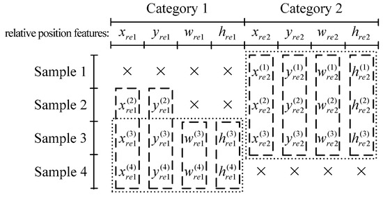
Figure 4.
A hypothetical simple case of missing values. A symbol “×” represents a missing value in the corresponding feature.
The decision tree algorithm used in the RF models is Classification and Regression Trees (CART) [36]. Decision tree classifiers and regressors are used to refine probabilities and coordinates respectively. In CART algorithm, a test sample’s refined coordinate is predicted to be the average of the training samples’ true coordinates in the corresponding leaf node. However, the box coordinates are continuous in images, so simply taking the average will discretize the coordinates and decrease the accuracy. To predict the coordinates more accurately, in each leaf node, we build a linear regression model with the training samples, and use it to predict the refined coordinates of the test samples. Take the refinement of coordinate x for example. Assume that there are r training samples in a leaf node, and the features of each training sample are 4 + 4k dimensions (4 dimensions of coordinates output by RPN or bounding-box regressor, and 4k dimensions of relative position features, explained in Section 4.1). Because the relative position features may contain missing values, we just extract the 4 dimensions of coordinates (i.e., x, y, w, h) and construct multivariable linear regression as:
where xrefine represents a refined coordinate, and a true coordinate x* of a train sample serves as its label (likewise for yrefine, wrefine, hrefine). The parameters b0 to b4 are fitted by the r training samples with the least square method. Based on the linear regression models in a leaf node, when a test sample with (4 + 4k)-dimensional features is assigned to the leaf node, its refined coordinates can be predicted as Equation (11).
4. Training and Detection Process
4.1. Training Process of Improved Faster R-CNN
The training process includes two parts. The first one is the training of the neural network, which modifies the four-step alternating training in [11] to suit the double feature maps. The second one is the training of the RF models, especially for various situations of feature value absence.
The training steps of the neural network are presented in Table 1 and Figure 5. In Table 1, all the initialization and reinitialization are carried out by an ImageNet-pre-trained model [39].

Table 1.
The training steps of the neural network.
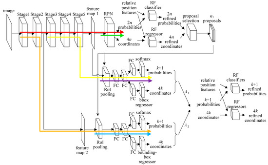
Figure 5.
The training process of the neural network.
After training the neural network, the training steps for the RF models are as follows:
Step 1: Generate several combinations based on all the ground-truth boxes of each training image, in order to consider various situations that some ground-truth boxes (components) have not been detected. Assume that there are m ground-truth boxes in an image (m = 1, 2, …, k), each of which may have been detected or not during the detection process, and then the total number of the combinations generated by all the ground-truth boxes in the image is:
It should be noted that all the combinations of an image are different from each other.
Step 2: Train the RF classifier in the proposal generation module. Through the trained ResNet-50 and RPN, an image will generate n proposals with two probabilities of containing an object or not containing an object. With 2m ground-truth box combinations, each proposal can generate 2m relative position feature vectors, so the image will produce n × 2m vectors of 2 + 4k dimensions (2 dimensions of probabilities and 4k dimensions of relative position features) for training. The training labels are the same as the probability labels in RPN training.
Step 3: Train the RF regressor in the proposal generation module like Step 2, but replace the two probabilities in the training vectors with the four coordinates generated by RPN. The training labels are the same as the coordinate labels in RPN training. According to the loss function of RPN in [11], the proposals with labels of not containing an object are not used in the RF regressor training.
Step 4: Train the RF classifiers in the category and position detection module. Each of the n1 proposals from the proposal generation module will generate k + 1 weighted probabilities of k component categories and a “background” category, and each component category needs a RF classifier. Meanwhile, with 2m ground-truth box combinations, each component category can generate 2m relative position feature vectors, so the image will produce n1 × 2m vectors of 1 + 4k dimensions (1 dimension of weighted probability and 4k dimensions of relative position features) for the training of each component category’s RF classifier. The training labels are the same as the probability labels in the softmax training. For the “background” category, there are no corresponding weighted coordinates for calculating the relative position features, and thus we take its weighted probability as its refined probability.
Step 5: Train the RF regressors in the category and position detection module like Step 4, but replace the one weighted probability in the training vectors with the four weighted coordinates. The training labels are the same as the coordinate labels in the bounding-box regressor training. According to the multi-task loss function in [10], for a proposal, if the probability label of a component category is 0, the proposal will not be used to train the RF regressor of this component category. Thus, similar to bounding-box regressors, the RF regressors just fine-tune the coordinates of the proposals.
4.2. Detection Process of Improved Faster R-CNN
After the training process, the improved Faster R-CNN model is used to detect transformer components, as shown in Algorithm 1. The statements with asterisks in Algorithm 1 will be explained in detail.
| Algorithm 1. Algorithm for transformer component detection |
| Input: an image, n1*, confidence_threshold* Output: a set final_boxes* containing k1 final box tuples (k1 = 0, 1, …, k), each of which contains a component category with a probability and 4 coordinates Input an image to ResNet-50 and generate feature map 1 and feature map 2 Initialize final_boxes to empty set While the number of elements in final_boxes < k do Input feature map 1 to proposal generation module* and generate n1 proposals Input n1 proposals, feature map 1 and feature map 2 to category and position detection module* and generate n1 × k box tuples (ignore the background category), each of which contains a category with a probability and 4 coordinates, and form a set boxes with n1 × k box tuples Delete all the box tuples whose categories already exist in final_boxes from boxes Select the box tuple with the highest probability in boxes as final_box If the probability of final_box < confidence_threshold then Break Else Append final_box to final_boxes End if End while |
The details of Algorithm 1 are as follows:
- The parameter n1 decides the number of the proposals selected into the category and position detection module; the parameter confidence_threshold decides the probability threshold of the output final box.
- Each final box in the set final_boxes frames a detected transformer component in the image, and provides its category and probability.
- The relative position features of a proposal in the proposal generation module or the category and position detection module are generated by the coordinates of the proposal and the final boxes.
5. Case Study
5.1. Data Set, Models and Indices
A total of 2000 main transformer inspection images, taken in 2016–2017 from a 220 kV substation in China, are selected as the data set for our experiment. The resolution of each image is 800 (width) × 600 (height). Parts of the images are shown in Figure A1. According to the type of the transformers in the data set, six categories of components are chosen to be detected, including the conservator, the #1–#9 radiator group, the #10–#18 radiator group, the gas relay, the breather of the main body, and the breather of on-load tap-changer (OLTC). Then, the positions of the six categories of components in the images are labeled with ground-truth boxes. In the experiment, we use 10-fold cross-validation (i.e., train on 1800 images and test on 200 images for 10 times in turn), and put the detected results of all the tested images (which are exactly the 2000 images in the data set) together to obtain statistics. In the data set, the amounts of the images containing different numbers of component categories, and the ones of the images containing each component category are shown in Table 2.

Table 2.
Statistics of images with different component category cases in the data set.
According to the experiments in [11], for the neural network of improved Faster R-CNN model (FRCNN-improved, for short), the number of proposals selected into the category and position detection module (i.e., n1) is set to 2000 and 300 in the training and test process respectively, and the anchors in RPN are of 4 sizes (82, 322, 1282, 5122) and 3 aspect ratios (2:1, 1:1, 1:2). We also use a learning rate of 0.003 and a mini-batch size of 8, and set the number of training steps as 50,000 by parameter optimization. For the RF models, the key parameters are shown in Table 3.

Table 3.
Key parameters of RF models.
To examine the effect of the two main improvements in FRCNN-improved, three models in Table 4 are used as controls, in which FRCNN-original is exactly the model in [11]. Compared with FRCNN-improved, FRCNN-v1 only adopts a single feature map output by Stage 5 of ResNet-50 in the category and position detection module, and the results produced by the softmax and bounding-box regressor are directly refined by RF models without a weighting process, while FRCNN-v2 omits the refinements with relative position features in both the proposal generation module and the category and position detection module, and takes the weighted probabilities and coordinates in the category and position detection module as the final results without an iterative refinement process. The parameters of the three models as controls are set in accordance with the corresponding ones in FRCNN-improved. Meanwhile, two recent object detection models, Cascade R-CNN [28] and YOLOv3 [25], as well as two classical models with relatively high accuracy, SSD [12] and R-FCN [13], are chosen for comparison. In addition, each image in the data set contains only one transformer, that is, each component category appears at most once in an image. Therefore, in all the detection models, for each category in an image, we only select a detected box with the highest probability as the final box.

Table 4.
The settings of the proposed model and the three models as controls.
A common index in object detection tasks, mean average precision (mAP), is evaluated in the experiment. Although mAP can reflect the accuracy of detection models in a relatively comprehensive perspective, it needs complicated calculation by repeatedly changing the parameter confidence_threshold to obtain several groups of precisions and recalls, and thus its engineering significance is not clear enough. To directly reflect the accuracy of the models in engineering application, the confidence_threshold is set to 0.6 by parameter optimization, and the precision and recall of each component category as well as the total precision and recall are evaluated. Additionally, the average detection time per image is calculated, which is measured on a Nvidia GeForce GTX 750 Ti GPU (NVIDIA, Santa Clara, CA, USA).
To determine whether a box frames a component correctly, the intersection over union (IoU) is adopted [11], which means the area ratio of the intersection of the box and the ground-truth box to the union of them. If IoU > 0.5, the box is judged as framing a component correctly.
5.2. Detection Results and Discussion
After training, the models are employed to detect the transformer components in the test images, and the detection results are shown in Table 5. As Table 5 shows, compared with the other models in Table 4, FRCNN-improved performs significantly better in the mAP and the total precision and recall, which are all over 94%. Thus, the two main improvements in the proposed model are both beneficial to raising the accuracy to a satisfactory level. Because the final boxes need to be generated iteratively in the detection process, the detection time of FRCNN-improved is the longest. However, the transformer inspection is a regular task without a high real-time requirement, while the efficiency of 2.1 s per image is obviously higher than the manual efficiency, so the proposed model is still significant for practical applications. Moreover, the accuracy of the four models based on Faster R-CNN is generally higher than that of YOLOv3, SSD and R-FCN, which indicates that Faster R-CNN is more suitable for transformer component detection. Similar to FRCNN-improved and FRCNN-v1, Cascade R-CNN adopts an iterative way to refine the predicted results, but its accuracy is lower mainly because its refinement is based on statistical results in ordinary object data sets, which is less effective and interpretable than the relative position features.

Table 5.
Statistical results of different models.
In addition, from the comparison of the precisions and recalls of specific component categories, it can be found that on the three relatively small components in Table 5 (i.e., gas relay, breather of main body, breather of OLTC), FRCNN-improved performs obviously better than FRCNN-v1, and similarly FRCNN-v2 performs better than FRCNN-original, which show that the models with double feature maps are better at detecting small objects than the corresponding single-feature-map models. Besides, on all the categories, the accuracy of the models with relative position features is higher than that of the corresponding models without relative position features, especially on the components with a similar appearance (i.e., the two categories of radiator groups, the two categories of breathers). To give more detailed explanations for these results, the two main improvements in the proposed model are analyzed in depth.
5.2.1. Double Feature Maps
The differences in the component sizes and the shooting distances lead to the great change of the object sizes in the images. In the data set, the largest ground-truth box is 227,454 pixels, while the smallest one is only 48 pixels. Moreover, small objects are more difficult to detect [23], so a low-level feature map is necessary. To verify the advantage of double feature maps in adapting to the change of object sizes, the sizes of all the ground-truth boxes in the data set are divided into five intervals according to the order of magnitude. Then, the recalls of the four Faster R-CNN based models in different size intervals are evaluated; the results are shown in Figure 6.
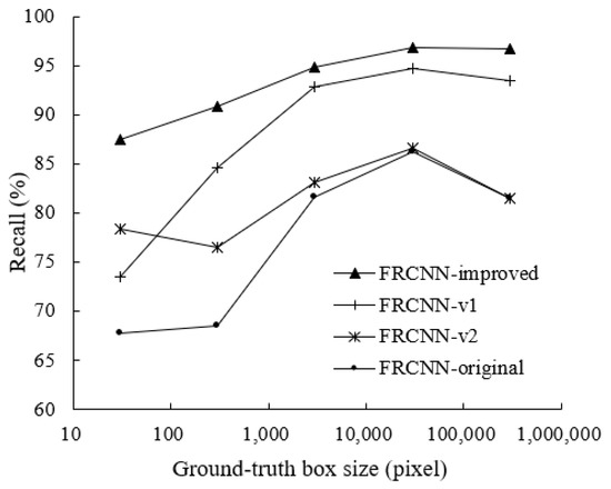
Figure 6.
Recalls of the four Faster R-CNN based models in different size intervals.
From the comparison of FRCNN-improved and FRCNN-v1 (or the comparison of FRCNN-v2 and FRCNN-original), it can be seen that the recalls of models with double feature maps are higher than the corresponding single-feature-map models, and the advantages are more obvious in smaller sizes. This is also why the models with double feature maps perform better on the three relatively small components in Table 5. The detection results of two images are shown in Figure 7 to give an intuitive illustration, in which the red boxes are the ground-truth boxes, the yellow boxes are the detection results of FRCNN-improved, and the blue boxes are the detection results of FRCNN-v1. In Figure 7a, FRCNN-v1 fails to detect the gas relay; in both the two images, the positions of breathers and gas relays detected by FRCNN-improved are more accurate.
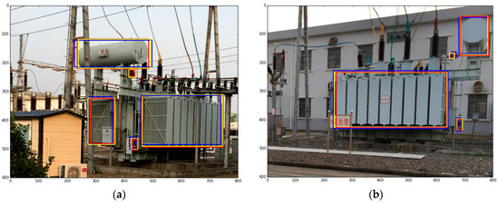
Figure 7.
Detection results of two test images. The categories and probabilities are not displayed for brevity. (a) A relatively frontal shooting angle; (b) A lateral shooting angle.
5.2.2. Relative Position Features
In the proposal generation module, with the relative position features between proposals and final boxes, the RF classifier can refine the proposal probabilities of containing an object or not containing an object (e.g., decrease the probability of containing an object if a proposal is far from the final boxes), while the RF regressor can refine the proposal coordinates by learning the proportion relations of the component sizes and positions. The detection process of FRCNN-improved is used to illustrate the advantage of relative position features. In the detection process of an image, as the number of iterations increases, more final boxes will be generated and thus more relative position features are available for proposal generation. Because a test image actually contains only 5 categories of components at most, the number of final boxes used in an iteration may be 0 to 4. Under each number of final boxes, the recall of the proposals output by the proposal generation module and the average IoU of the “correct” (i.e., IoU > 0.5) proposals are evaluated, as shown in Figure 8.
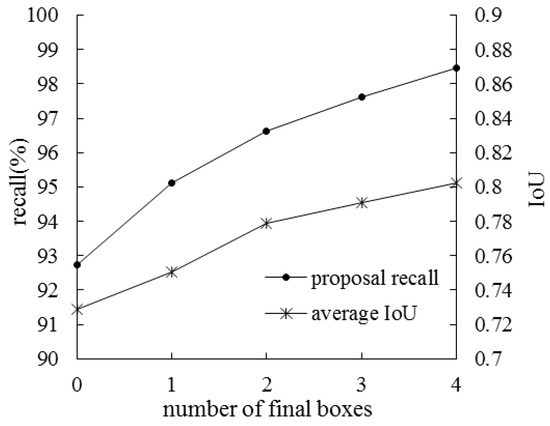
Figure 8.
Proposal recalls and average intersection over union (IoU) under different numbers of final boxes.
It can be seen from Figure 8 that as the number of final boxes increases (i.e., the number of relative position features increases), the recall of the proposals is improved, which indicates that the probabilities of the proposals are more accurate. Meanwhile, the average IoU is higher with more final boxes, which suggests that the accuracy of the proposal coordinates is improved.
In the category and position detection module, the RF models’ refinement principles are similar to that of the proposal generation module, but the refinement is aimed at specific categories of components. Intuitive explanations are given in the two images in Figure 9. In both the images, we set that the #1–#9 radiator group and the #10–#18 radiator group have been detected, as the red boxes show. Then, in Figure 9a, we evenly select 4 × 7 boxes (the green boxes) of the same size as the breather of OLTC, and set that each box’s probability of containing a breather of OLTC is predicted to be 60.0% (the value of confidence_threshold) by the softmax classifier. After that, the probability and the position features relative to two radiator groups of each green box are input to the RF classifier, which then outputs the refined probabilities of containing a breather of OLTC, as the labels over the green boxes show. The refined probabilities indicate that, even if the neural network cannot distinguish the probabilities of different boxes, the RF classifier can still refine the probability of each box effectively through the relative position information, and select the correct final box with the highest probability.
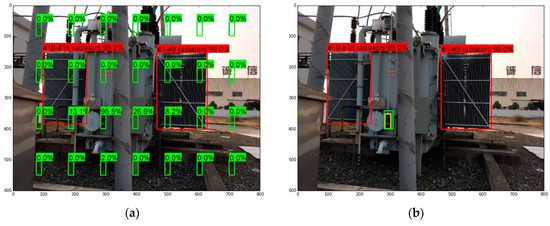
Figure 9.
Two examples for illustrating the effect of relative position features. (a) The refinement of probabilities; (b) The refinement of coordinates.
In Figure 9b, we set that the position of the breather of OLTC predicted by the bounding-box regressor is shown as the green box. Then, the coordinates and the position features relative to two radiator groups of the green box are input to the RF regressor, which then outputs the refined coordinates denoting the final box of the breather of OLTC, as the yellow box shows. Compared with the green box, the yellow box refined by the RF regressor is more accurate in the position and the size, which suggests that the coordinates can be refined with the aid of relative position features.
Therefore, in Table 5, the components with a similar appearance, which are easy to be confused when merely detected by the neural network, can be effectively distinguished by the RF models according to the relative position features. For the other components, the relative position features can also provide useful information of the proportion relations between components for the refinement, which will also improve the accuracy of detection.
6. Conclusions
To realize the automatic detection of transformer components in inspection images, an improved Faster R-CNN model is proposed in this paper, considering the difference in component sizes and the relative position information between components. The case study shows that the model significantly improves the accuracy of transformer component detection, which has evident practicability. It should be noted that all of the features used in the model, including those used by the neural network and the RF models, do not require manual construction for specific components. Therefore, the model is available for the component detection of various types of transformers and even other power equipment.
Our future work is to realize the automatic state recognition of transformers, of which the foundation is provided by the accurate detection of the categories and positions of various transformer components. Based on the detection results, the recognition algorithms need to be designed for different types of defects and faults related to transformers, which is also an important direction in our further research.
Author Contributions
Conceptualization, Z.L. and H.W.; methodology, Z.L.; software, H.W.; validation, Z.L.; formal analysis, H.W.; investigation, H.W.; resources, H.W.; data curation, H.W.; writing—original draft preparation, Z.L.; writing—review and editing, Z.L. and H.W.; visualization, Z.L. and H.W.; supervision, H.W.; project administration, H.W.; funding acquisition, H.W.
Funding
This research received no external funding.
Conflicts of Interest
The authors declare no conflict of interest.
Appendix A
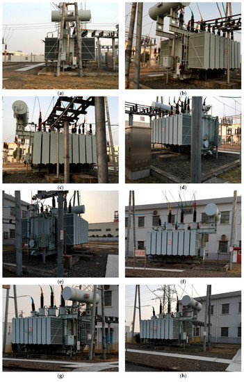
Figure A1.
Parts of the images in the data set. (a) A frontal shooting angle; (b) A relatively frontal shooting angle; (c) A lateral shooting angle; (d) A relatively back shooting angle; (e) A relatively back shooting angle; (f) A lateral shooting angle; (g) A relatively frontal shooting angle; (h) A relatively frontal shooting angle.
References
- Chen, H.; Zhao, X.; Zhao, X.; Tan, M. Computer vision-based detection and state recognition for disconnecting switch in substation automation. Int. J. Robot. Autom. 2017, 32, 1–12. [Google Scholar] [CrossRef]
- Yan, B.; Chen, H.; Huang, W. Study on the method of switch state detection based on image recognition in substation sequence control. In Proceedings of the 2014 International Conference on Power System Technology (POWERCON 2014), Chengdu, China, 20–22 October 2014; pp. 2504–2510. [Google Scholar] [CrossRef]
- Sun, L. Research on Practical Image Recognition Method of Abnormal Phenomenon of Electric Equipments in Substation. Master’s Thesis, North China Electric Power University, Beijing, China, March 2015. [Google Scholar]
- Bharata Reddy, M.J.; Chandra, B.K.; Mohanta, D.K. A DOST based approach for the condition monitoring of 11 kV distribution line insulators. IEEE Trans. Dielectr. Electr. Insul. 2011, 18, 588–595. [Google Scholar] [CrossRef]
- Wang, T.; Yao, C.; Liu, J.; Chao, L.; Shao, G.; Qun, H.; Ming, Y. Research on automatic identification of substation circuit breaker based on shape priors. Appl. Mech. Mater. 2014, 511–512, 923–926. [Google Scholar] [CrossRef]
- Lowe, D.G. Distinctive image features from scale-invariant keypoints. Int. J. Comput. Vis. 2004, 60, 91–110. [Google Scholar] [CrossRef]
- Dalal, N.; Triggs, B. Histograms of oriented gradients for human detection. In Proceedings of the IEEE Computer Society Conference on Computer Vision and Pattern Recognition, San Diego, CA, USA, 20–25 June 2005; pp. 886–893. [Google Scholar] [CrossRef]
- Shao, J.; Yan, Y.; Qi, D. Substation switch detection and state recognition based on Hough forests. Autom. Electr. Power Syst. 2016, 40, 115–120. [Google Scholar] [CrossRef]
- Girshick, R.; Donahue, J.; Darrell, T.; Malik, J. Rich feature hierarchies for accurate object detection and semantic segmentation. In Proceedings of the IEEE Conference on Computer Vision and Pattern Recognition, Columbus, OH, USA, 24–27 June 2014; pp. 580–587. [Google Scholar] [CrossRef]
- Girshick, R. Fast R-CNN. In Proceedings of the IEEE International Conference on Computer Vision, Santiago, Chile, 13–16 December 2015; pp. 1440–1448. [Google Scholar] [CrossRef]
- Ren, S.; He, K.; Girshick, R.; Sun, J. Faster R-CNN: Towards real-time object detection with region proposal networks. IEEE Trans. Pattern Anal. Mach. Intell. 2017, 39, 1137–1149. [Google Scholar] [CrossRef]
- Liu, W.; Anguelov, D.; Erhan, D.; Szegedy, C.; Reed, S.; Fu, C.; Berg, A.C. SSD: Single shot multibox detector. In Proceedings of the European Conference on Computer Vision, Amsteram, The Netherlands, 11–14 October 2016; pp. 21–37. [Google Scholar] [CrossRef]
- Dai, J.; Li, Y.; He, K.; Sun, J. R-FCN: Object detection via region-based fully convolutional networks. In Proceedings of the 30th Conference on Neural Information Processing Systems (NIPS 2016), Barcelona, Spain, 5–10 December 2016; pp. 379–387. [Google Scholar]
- Lin, T.Y.; Dollar, P.; Girshick, R.; He, K.; Hariharan, B.; Belongie, S. Feature pyramid networks for object detection. In Proceedings of the IEEE Conference on Computer Vision and Pattern Recognition, Honolulu, HI, USA, 21–26 July 2017; pp. 936–944. [Google Scholar] [CrossRef]
- Zhou, Q.; Zhao, Z. Substation equipment image recognition based on SIFT feature matching. In Proceedings of the 2012 5th International Congress on Image and Signal Processing (CISP 2012), Chongqing, China, 16–18 October 2012; pp. 1344–1347. [Google Scholar] [CrossRef]
- Chen, A.; Le, Q.; Zhang, Z.; Sun, Y. An image recognition method of substation breakers state based on robot. Autom. Electr. Power Syst. 2012, 36, 101–105. [Google Scholar]
- Chen, H.; Sun, S.; Wang, T.; Zhao, X.; Tan, M. Automatic busbar detection in substation: Using directional Gaussian filter, gradient density, Hough transform and adaptive dynamic K-means clustering. In Proceedings of the 34th Chinese Control Conference, Hangzhou, China, 28–30 July 2015; pp. 4668–4672. [Google Scholar] [CrossRef]
- Wang, J.; Wang, J.; Shao, J.; Li, J. Image recognition of icing thickness on power transmission lines based on a least squares Hough transform. Energies 2017, 10, 415. [Google Scholar] [CrossRef]
- Li, Z.; Liu, Y.; Walker, R.; Hayward, R.; Zhang, J. Towards automatic power line detection for UAV surveillance system using pulse coupled neural filter and Hough transform. Mach. Vis. Appl. 2010, 21, 677–686. [Google Scholar] [CrossRef]
- Zhao, Z.; Zhang, L.; Qi, Y.; Shi, Y. A generation method of insulator region proposals based on edge boxes. Optoelectron. Lett. 2017, 13, 466–470. [Google Scholar] [CrossRef]
- Sermanet, P.; Eigen, D.; Zhang, X.; Mathieu, M.; Fergus, R.; Lecun, Y. Overfeat: Integrated recognition, localization and detection using convolutional networks. In Proceedings of the International Conference on Learning Representations, Banff, AB, Canada, 14–16 April 2014; pp. 1–16. [Google Scholar] [CrossRef]
- Bell, S.; Zitnick, C.L.; Bala, K.; Girshick, R. Inside-Outside Net: Detecting objects in context with skip pooling and recurrent neural networks. In Proceedings of the IEEE Conference on Computer Vision and Pattern Recognition, Las Vegas, NV, USA, 27–30 June 2016; pp. 2874–2883. [Google Scholar] [CrossRef]
- Kong, T.; Yao, A.; Chen, Y.; Sun, F. Hypernet: Towards accurate region proposal generation and joint object detection. In Proceedings of the IEEE Conference on Computer Vision and Pattern Recognition, Las Vegas, NV, USA, 27–30 June 2016; pp. 845–853. [Google Scholar] [CrossRef]
- Wang, X.; Ma, H.; Chen, X.; You, S. Edge preserving and multi-scale contextual neural network for salient object detection. IEEE Trans. Image Process. 2018, 27, 121–134. [Google Scholar] [CrossRef]
- Redmon, J.; Farhadi, A. YOLOv3: An Incremental Improvement. Available online: https://pjreddie.com/media/files/papers/YOLOv3.pdf (accessed on 1 November 2018).
- Redmon, J.; Divvala, S.; Girshick, R.; Farhadi, A. You only look once: Unified, real-time object detection. In Proceedings of the IEEE Conference on Computer Vision and Pattern Recognition, Las Vegas, NV, USA, 27–30 June 2016; pp. 779–788. [Google Scholar] [CrossRef]
- Zhou, P.; Ni, B.; Geng, C.; Hu, J.; Xu, Y. Scale-transferrable object detection. In Proceedings of the IEEE Conference on Computer Vision and Pattern Recognition, Salt Lake City, UT, USA, 19–21 June 2018; pp. 528–537. [Google Scholar]
- Cai, Z.; Vasconcelos, N. Cascade R-CNN: Delving into high quality object detection. In Proceedings of the IEEE Conference on Computer Vision and Pattern Recognition, Salt Lake City, UT, USA, 19–21 June 2018. [Google Scholar]
- Cheng, B.; Wei, Y.; Shi, H.; Feris, R.; Xiong, J.; Huang, T. Revisiting RCNN: On awakening the classication power of Faster RCNN. In Proceedings of the European Conference on Computer Vision, Munich, Germany, 8–14 September 2018. [Google Scholar]
- Jiang, B.; Luo, R.; Mao, J.; Xiao, T.; Jiang, Y. Acquisition of localization confidence for accurate object detection. In Proceedings of the European Conference on Computer Vision, Munich, Germany, 8–14 September 2018. [Google Scholar]
- Chen, Y.; Li, W.; Sakaridis, C.; Dai, D.; Gool, L.V. Domain adaptive Faster R-CNN for object detection in the wild. In Proceedings of the IEEE Conference on Computer Vision and Pattern Recognition, Salt Lake City, UT, USA, 19–21 June 2018. [Google Scholar]
- Liu, S.; Huang, D.; Wang, Y. Receptive Field Block Net for accurate and fast object detection. In Proceedings of the European Conference on Computer Vision, Munich, Germany, 8–14 September 2018. [Google Scholar]
- Szegedy, C.; Ioffe, S.; Vanhoucke, V.; Alemi, A.A. Inception-v4, Inception-ResNet and the impact of residual connections on learning. In Proceedings of the Thirty-First AAAI Conference on Artificial Intelligence, San Francisco, CA, USA, 4–10 February 2017; pp. 4278–4284. [Google Scholar]
- He, K.; Zhang, X.; Ren, S.; Sun, J. Deep residual learning for image recognition. In Proceedings of the IEEE Conference on Computer Vision and Pattern Recognition, Las Vegas, CA, USA, 27–30 June 2016; pp. 770–778. [Google Scholar] [CrossRef]
- Russell, S.J.; Norvig, P. Making simple decisions. In Artificial Intelligence: A Modern Approach, 2nd ed.; Pompili, M., Chavez, S., Eds.; Alan Apt: Englewood Cliffs, NJ, USA, 2003; Volume 5, pp. 471–497. ISBN 0-13-103805-2. [Google Scholar]
- Breiman, L.; Friedman, J.H.; Olshen, R.A.; Stone, C.J. Classification and Regression Trees; CRC Press: Boca Raton, FL, USA, 1998; ISBN 0-412-04841-8. [Google Scholar]
- Quinlan, J.R. C4.5: Programs for Machine Learning; Morgan Kaufmann Publishers: San Mateo, CA, USA, 1993; ISBN 1-55860-238-0. [Google Scholar]
- Brodley, C.E.; Utgoff, P.E. Multivariate decision trees. Mach. Learn. 1995, 19, 45–77. [Google Scholar] [CrossRef]
- Russakovsky, O.; Deng, J.; Su, H.; Krause, J.; Satheesh, S.; Ma, S.; Huang, Z.; Karpathy, A.; Khosla, A.; Bernstein, M.; et al. ImageNet large scale visual recognition challenge. Int. J. Comput. Vis. 2015, 115, 211–252. [Google Scholar] [CrossRef]
© 2018 by the authors. Licensee MDPI, Basel, Switzerland. This article is an open access article distributed under the terms and conditions of the Creative Commons Attribution (CC BY) license (http://creativecommons.org/licenses/by/4.0/).
