Theoretical Analysis of Planar Spiral Coils between Two Multilayer Media for Electric Vehicle Wireless Charging

Abstract

Square and circular coils are two typical topologies for coupling coils and are applied to wireless charging. However, most of the research on coupling coils is based on the finite element model (FEM), which is a time-consuming process for 3-D structure coils. In this paper, on the basis of Fourier–Bessel transformation and Dual Fourier transformation, two theoretical models of square and circular coils between two multilayer media are proposed. With the proposed models, we consider several important parameters such as the size of the coils, thickness, and permeability of each layer. Thus, both the self-inductance and mutual inductance of two planar coils can be calculated without much computational time. Additionally, these theoretical models can help designers figure out the different trends of self-inductance and mutual inductance, which has plenty of benefits for the preliminary pad design. Lastly, a prototype with a size of 600 mm × 600 mm and a 200 mm air gap was built in order to verify the proposed models.

1. Introduction

Due to the fossil energy crisis and greenhouse gas limitations, electric vehicles including pure electric or hybrid power vehicles, have been promoted in recent years. The battery is commonly known as one of the most important components in an electric vehicle. Fuel cell and lithium-ion batteries are the most commonly used power sources in electric vehicles. Each type of battery has its own idiosyncrasy. For example, fuel cell systems [1], which have high power density and high efficiency faces obstacles of producing, transporting, and storing hydrogen. The lithium-ion battery [2,3], on the other hand, is relatively cheap and requires low maintenance. However, it has an aging problem and low performance in high or low temperature environments. Additionally, the conventional charging method used by wires is also a risky and painstaking operation for users who own electric vehicles. Wireless power transfer (WPT) is an emerging technology that has been a hot area of research [4,5,6,7,8,9] in recent years due to its safety and convenience when compared with plug-in charging or fuel cell systems for electric vehicles. WPT produces no contaminants and is completely reliable and maintenance-free unlike conventional plug-in or brush and bar contact-based methods.

In general, as shown in Figure 1, a typical WPT system includes a power source, a power factor correction circuit, an H Bridge inverter, an excited coil, a pick-up coil, a rectifier, a filter, and the battery [10]. In this system scheme, the power factor correction circuit is a conversion facility that outputs the DC power supply from the power electricity grid. After that, the H Bridge is used to convert the current from DC to AC, which is necessary to excite a magnetic field by the excited coil. In contrast, the rectifier filter acts as an AC/DC converter because only DC is suitable for battery charging.

In Figure 1, the coupled coil design is a crucial and indispensable part of a WPT system. For coupled coil investigation, one of the most important parameters is mutual inductance between the excited coil and the pick-up coil. In order to estimate the mutual inductance, we need to determine the coil geometries first. So far, circular and square coil geometries have been most widely used [11,12,13,14,15,16]. In some work, mutual inductance for circular coils is calculated by using approximated formulas [14,17,18]. The circular geometry has cylindrical symmetry, and the theoretical model is relatively straightforward since only a ρ-component exists in the spatial vector potential. On the other hand, square and rectangular coil geometries have been found to be well-suited for mid-distance WPT systems [19,20]. Recently, some scholars have paid studied these coil geometries analysis by finite element model (FEM) simulation [21,22,23,24]. However, few scholars have investigated in detail an effective and efficient theoretical model to calculate the self-inductance and mutual inductance when magnetic shielding layers are added to the pad. In order to obtain the magnetic field distribution between two multilayer media, several partial differential equations (PDEs) must be solved. Therefore, Fourier–Bessel transformation and Dual-Fourier transformation are proposed to calculate the solution of these PDEs. With the theoretical model, the magnetic field distribution of some complex pad structures such as double D pad [25] or compound pad design [26] can also be calculated theoretically with less computational time.

This paper follows prior work [27]. The main contribution of this particular paper is the study of the multi-layer media. In practical usage, the coupling pad in the WPT system should include several layers. Beside the ferrite layer, an additional metallic layer should also be added in order to ensure that the electrical component in the vehicle cannot be interfered with by the leaking magnetic flux and that extra heat loss can be avoided in the metallic components in the chassis. Therefore, it is essential to build a theoretical model of multi-layer media of the pads, which is closer to our pragmatic application. If the solution obtained in [27] is used directly in this case, the expression of the magnetic flux distribution will be very cumbersome. As such, it is necessary to change the form of the equations in each region so as to apply for the matrix, which can greatly simplify the derivation of the theoretical model. Furthermore, this paper also presents several promising studies, which can provide guidance for the pad designers.

This paper is mainly divided in three parts. First, an analytical approach to calculate the mutual inductance and self-inductance of circular and square coils between two multilayer media is described. Then, preliminary investigations using the proposed models are reported so as to demonstrate their utility for pad design. Lastly, the influence of lateral misalignment of circular and square coils is explained, and an experimental prototype to validate the theoretical models is described.

2. Theoretical Model of Planar Spiral Coils between Two Multilayer Media

In this section, several magnetic field theoretical models of both circular and square coils are proposed in order to obtain the self-inductance and mutual inductance. All of these models are excited by the time-harmonic current. Given that the coils are wrapped by litz wires, the skin effect can be neglected with relative low operating frequencies varied from 80 to 100 kHz [27]. On the assumption that the coils can be regarded as filaments, the magnitude of B-field is calculated via magnetic vector potential.

2.1. Mutual Inductance of Circualr Coils with Two Multilayer Media

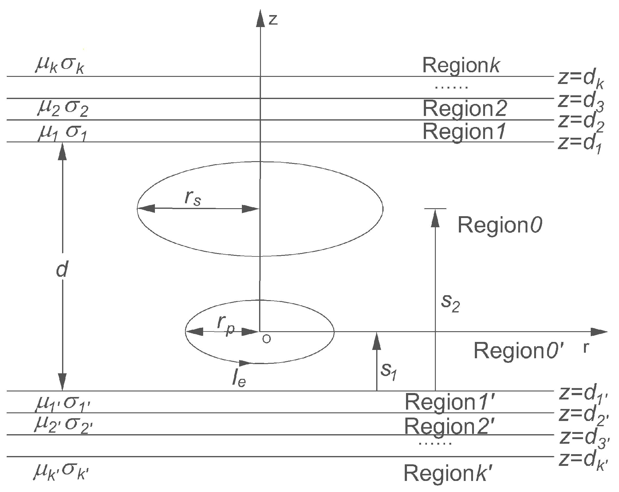
In the cylindrical coordinate shown in Figure 2, a k-layer medium is located at a coordinate d₁ above the pick-up circular filament with radius of r_s. The layers are numbered from 1 to k in an upward direction. Another k’-layer medium, of which layers are numbered from 1’ to k’ in a downward direction, is placed beneath the excited circular filament with radius of r_p, which occupies the region z ≤ d_1’. Each region of the multilayer medium has a thickness $t_k=\left|d_{k+1}-d_k\right|$ except regions k and k’, which are considered semi-infinite. d is the distance between the upper surface of the multilayer media and the lower surface of the upper multilayer media. Each region is homogeneous and isotropic with an electrical conductivity σ_k and a relative permeability µ_k.

The magnetic field is produced by the sinusoidal current $i_e=I_e{e}^{j\omega t}$ in the primary coil at z = s₁. On the hypothesis that the displacement current is neglected, it is easy to obtain Poisson’s equation by using the Coulomb gauge condition.

$${\nabla }^2\overrightarrow{A}=-\mu J_e$$

(1)

where J_e is the current density, and A is the magnetic vector potential.

On the basis of the Maxwell equations and cylindrical symmetry, the magnetic vector potential only has an e_φ-component and the PDEs of each regions are shown in the following expressions [28]:

Regions 1 to k and 1’ to k’ are expressed as

$$\frac{{\partial }^2{A}_{\varphi ,k}}{\partial z^2}+\frac{{\partial }^2{A}_{\varphi ,k}}{\partial r^2}+\frac{1}{r}\frac{\partial A_{\varphi ,k}}{\partial r}-(\frac{1}{r^2}+j\omega {\mu }_0{\mu }_k{\sigma }_k)A_{\varphi ,k}=0$$

(2)

and regions 0 and 0’ are expressed as

$$\frac{{\partial }^2{A}_{\varphi ,k}}{\partial z^2}+\frac{{\partial }^2{A}_{\varphi ,k}}{\partial r^2}+\frac{1}{r}\frac{\partial A_{\varphi ,k}}{\partial r}-\frac{A_{\varphi ,k}}{r^2}+{\mu }_0{I}_e\delta (r-r_p)\delta (z)=0.$$

(3)

where ${\mu }_0$ is the constant of permeability of vacuum, and I_e is the magnitude of time-harmonic current. A_Φ,k is the e_φ-component of the magnetic vector potential in each region. $\delta (x)$ is defined as follows:

$$\{\begin{array}{c}\delta \left(x\right)=0\left(x\ne 0\right)\\ \delta \left(x\right)=1\left(x=0\right)\end{array}.$$

Based on the Fourier–Bessel transform [29], the one-dimensional transformed versions of Equations (2) and (3) are obtained.

Regions 1 to k and 1’ to k’ are expressed as

$$\frac{{\partial }^2{A}_{\varphi ,k}^{*}}{\partial z^2}=({\gamma }^2+j\omega {\mu }_k{\sigma }_k)A_{\varphi ,k}^{*}.$$

(4)

Regions 0 and 0’ are expressed as

$$\frac{{\partial }^2{A}_{\varphi ,k}^{*}}{\partial z^2}={\gamma }^2{A}_{\varphi ,k}^{*}-{\mu }_0{I}_e{r}_p{J}_1(\gamma r_p)\delta (z).$$

(5)

The general solution for each region is seen in Equation (6):

$$A_{\varphi ,k}^{*}(\gamma ,z)=C_k{e}^{-{\eta }_k(z-d_k)}+D_k{e}^{{\eta }_k(z-d_k)}$$

(6)

where 𝜂_k is a complex parameter that depends on frequency and material properties of each region:

$${\eta }_k=\sqrt{{\gamma }^2+j\omega {\mu }_{rk}{\mu }_0{\sigma }_k}.$$

(7)

Then, according to the boundary conditions that hold at the position of the coil and at the interface of the adjacent regions, the 2(k + k’) + 2 unknown coefficients are obtained.

At the position of the excited filament (z = 0), E_φ is continuous and H_r is discontinuous, which equals the surface current density of the excited filament:

$$\begin{gathered} A_{\varphi ,0}^{*}(z=0)=A_{\varphi ,0^{\prime }}^{*}(z=0) \\ \frac{1}{{\mu }_0}\frac{\partial A_{\varphi ,0}^{*}}{\partial z}(z=0)-\frac{1}{{\mu }_0}\frac{\partial A_{\varphi ,0^{\prime }}^{*}}{\partial z}(z=0)=-I_{\varphi }{r}_p{J}_1(\gamma r_p). \end{gathered}$$

(8)

The above Equation (5) can be also rewritten in matrix notation:

$$\left(\begin{array}{c}{D}_0\\ C_0\end{array}\right)-\left(\begin{array}{c}{D}_{0\prime }\\ C_{0\prime }\end{array}\right)=\frac{{\mu }_0{I}_e{r}_p{J}_1(\gamma r_p)}{2\gamma }\left(\begin{array}{c}-1\\ 1\end{array}\right).$$

(9)

At the interface of the regions k and k − 1(z = d_k), both E_φ and H_r are continuous:

$$\begin{gathered} A_{\varphi ,k}^{*}(z=d_k)=A_{\varphi ,k-1}^{*}(z=d_{k-1}) \\ \frac{1}{{\mu }_k}\frac{\partial A_{\varphi ,k}^{*}}{\partial z}(z=d_k)=\frac{1}{{\mu }_{k-1}}\frac{\partial A_{\varphi ,k-1}^{*}}{\partial z}(z=d_{k-1}). \end{gathered}$$

(10)

Equation (4) can be expressed in matrix notation:

$${\Re }_{\mathrm{k},\mathrm{k}-1}\left(\begin{array}{c}{D}_k\\ C_k\end{array}\right)-I\left(\begin{array}{c}{D}_{k-1}\\ C_{k-1}\end{array}\right)=0$$

(11)

where I is the identity matrix of order 2, and ${\Re }_{k.k-1}$ is the following square matrix of order 2:

$${\Re }_{\mathrm{k},\mathrm{k}-1}=\frac{1}{2}\left(\begin{array}{cc}(1+\frac{{\zeta }_k}{{\zeta }_{k-1}})e^{-{\eta }_{k-1}{t}_{k-1}}& (1-\frac{{\zeta }_k}{{\zeta }_{k-1}})e^{-{\eta }_{k-1}{t}_{k-1}}\\ (1-\frac{{\zeta }_k}{{\zeta }_{k-1}})e^{{\eta }_{k-1}{t}_{k-1}}& (1+\frac{{\zeta }_k}{{\zeta }_{k-1}})e^{{\eta }_{k-1}{t}_{k-1}}\end{array}\right)$$

(12)

where ζ_k = 𝜂_k/µ_k, and t_k is the thickness of the nth region.

Because the magnetic vector potential tends to be zero when z approaches positive infinity and negative infinity, both D_k and C_k’ are zero. Therefore, ${\Re }_{k.k-1}$ and ${\Re }_{k^{\prime }.k^{\prime }-1}$ are matrices of dimension 2 × 1:

$$\begin{gathered} {\Re }_{k,k-1}=\frac{1}{2}\left(\begin{array}{c}(1-\frac{{\zeta }_k}{{\zeta }_{k-1}})e^{-{\eta }_{k-1}{t}_{k-1}}\\ (1+\frac{{\zeta }_k}{{\zeta }_{k-1}})e^{{\eta }_{k-1}{t}_{k-1}}\end{array}\right) \\ {\Re }_{k^{\prime },k^{\prime }-1}=\frac{1}{2}\left(\begin{array}{c}(1+\frac{{\zeta }_{k^{\prime }}}{{\zeta }_{k^{\prime }-1}})e^{-{\eta }_{k^{\prime }-1}{t}_{k^{\prime }-1}}\\ (1-\frac{{\zeta }_{k^{\prime }}}{{\zeta }_{k^{\prime }-1}})e^{{\eta }_{k^{\prime }-1}{t}_{k^{\prime }-1}}\end{array}\right). \end{gathered}$$

(13)

From Equations (9) and (14), it is easy to obtain the calculations below.

$$\begin{gathered} \left(\begin{array}{c}{D}_0\\ C_0\end{array}\right)=({\displaystyle \prod _1^k{\Re }_{k,k-1})C_k} \\ \left(\begin{array}{c}{D}_{0^{\prime }}\\ C_{0^{\prime }}\end{array}\right)=({\displaystyle \prod _{1^{\prime }}^{k^{\prime }}{\Re }_{k,k-1})D_{k^{\prime }}}. \end{gathered}$$

(14)

According to Equations (9) and (14), all of the unknown coefficients can be calculated. In terms of the mutual inductance, only D₀ and C₀ need to be calculated.

In order to compute the mutual inductance of the coils, the total voltage amplitude induced at the pick-up coil (z = s₂ − s₁) must be evaluated. It is calculated in Equation (15):

$$V=j\omega {\displaystyle \underset{pcik-up}{\oint }{A}_{\varphi }·dl=}j\omega {\displaystyle {\int }_0^{2\pi }{A}_{\varphi }(r=r_s,z=s_2-s_1)}{r}_{s}d\varphi .$$

(15)

Then

$$M=\mathrm{Im}(\frac{V}{I_e})/\omega$$

(16)

where Im is the function used for extracting the imaginary part of a complex number.

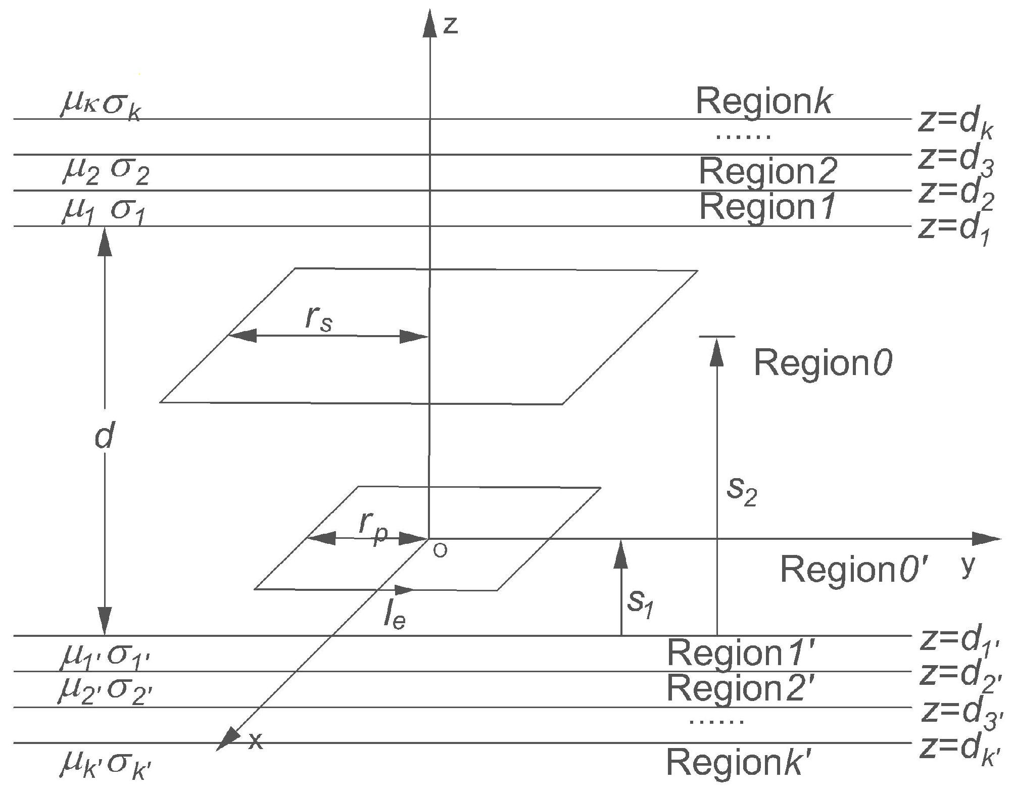
2.2. Mutual Inductance of Square Coils with Two Multilayer Media

The basic structure of a theoretical model is depicted in Figure 3. In this figure, all of the parameters are the same as the definition in Figure 2.

As for rectangular coils, it is more complicated to establish its math model by several PDEs due to its non-cylindrical symmetry feature. Before the whole system’s model is set up, it is necessary to determine the magnetic flux density distribution of the two rectangular coils in the air first.

In regions 0 and 0’, the magnetic flux density B can be divided into two parts. B_i is excited by the current flowing in the primary coil and B_r is produced by the induced eddy current.

The first step is to calculate the B_i-field. According to the relationship between the magnetic flux density and the magnetic vector potential, the magnetic vector potential of arbitrary point p(x,y,z) can be derived by integrating the source point (x’,y’,z’) as seen in Equation (17) below:

$$A(x,y,z)=\frac{{\mu }_0}{4\pi }{\displaystyle \underset{s}{\int }\frac{J(x^{\prime },y^{\prime },z^{\prime })d{s}^{\prime }}{R}}$$

(17)

where J is the current density and s is the current distribution of an excited coil. The distance between p(x,y,z) and source point (x’,y’,z’) is denoted by R.

In order to solve Equation (17), the Dual Fourier Transformation and its inverse method are applied [30], and the z-component of the B_i-field of spatial frequency domain can be obtained:

$$b_{iz}^{\prime }=\frac{-2{\mu }_0{I}_e\gamma \sin (r_p\alpha )\sin (r_p\beta )}{\alpha \beta }{e}^{z\gamma }=C_{iz}^{\prime }{e}^{z\gamma }$$

(18)

$$b_{iz}=\frac{-2{\mu }_0{I}_e\gamma \sin (r_p\alpha )\sin (r_p\beta )}{\alpha \beta }{e}^{-z\gamma }=C_{iz}{e}^{-z\gamma }.$$

(19)

As for the B_r-field, it can be calculated using the following equations.

$${\nabla }^2\overrightarrow{B_r}=0$$

(20)

$$\nabla ·\overrightarrow{B_r}=0.$$

(21)

By applying the Dual Fourier Transformation, the z-component of the B_r-field of the spatial frequency domain in regions 0 and 0’ can be expressed as Equations (22) and (23) below:

$$b_{z,0}=(C_{iz}+C_{rz}^{\prime })e^{-\gamma z}+C_{rz}{e}^{\gamma z}$$

(22)

$$b_{z,0\prime }=(C_{iz}^{\prime }+C_{rz})e^{\gamma z}+C_{rz}^{\prime }{e}^{-\gamma z}$$

(23)

Similar to the B_r-field calculation in regions 0 and 0’, the z-component of the B_r-field of spatial frequency domain can also be obtained:

$$b_{z,k}=C_{z,k}{e}^{{\eta }_k(z-d_k)}+C_{z,k}^{\prime }{e}^{-{\eta }_k(z-d_k)}$$

(24)

where ${\eta }_k=\sqrt{{\gamma }^2+j\omega {\mu }_{rk}{\mu }_0{\sigma }_k}.$

Then based on the boundary conditions, at the interface of regions k and k − 1, the z-component of B and the x-component of H must be continuous except at the position z = 0:

$$b_{z,k}=b_{z,k-1}(z=d_k)$$

(25)

$$b_{x,k}/{\mu }_k=b_{x,k-1}/{\mu }_{k-1}(z=d_k).$$

(26)

The resulting equations can be rewritten in matrix notation:

At z = d₁,

$${\Re }_{1,0}\left(\begin{array}{c}{C}_{z,1}\\ C_{z,1}^{\prime }\end{array}\right)-I\left(\begin{array}{c}{C}_{rz}\\ C_{iz}+C_{rz}^{\prime }\end{array}\right)=0$$

(27)

At z = d_1’,

$${\Re }_{1\prime ,0\prime }\left(\begin{array}{c}{C}_{z,1^{\prime }}\\ C_{z,1^{\prime }}^{\prime }\end{array}\right)-I\left(\begin{array}{c}{C}_{rz}+C_{iz}^{\prime }\\ C_{rz}^{\prime }\end{array}\right)=0$$

(28)

At z = d_k (n = 2~k and 2’~k’),

$${\Re }_{k,k-1}\left(\begin{array}{c}{C}_{z,k}\\ C_{z,k}^{\prime }\end{array}\right)-I\left(\begin{array}{c}{C}_{z,k-1}\\ C_{z,k-1}\end{array}\right)=0$$

(29)

I is the identity matrix of order 2 and ${\Re }_{k.k-1}$ is the following square matrix of order 2.

$${\Re }_{k,k-1}=\frac{1}{2}\left(\begin{array}{cc}(1+\frac{{\zeta }_k}{{\zeta }_{k-1}})e^{-{\eta }_{k-1}{t}_{k-1}}& (1-\frac{{\zeta }_k}{{\zeta }_{k-1}})e^{-{\eta }_{k-1}{t}_{k-1}}\\ (1-\frac{{\zeta }_k}{{\zeta }_{k-1}})e^{{\eta }_{k-1}{t}_{k-1}}& (1+\frac{{\zeta }_k}{{\zeta }_{k-1}})e^{{\eta }_{k-1}{t}_{k-1}}\end{array}\right).$$

(30)

Since the magnetic vector potential tends to be zero when z approaches positive infinity and negative infinity, both D_k and C_k’ are zero, which is similar to the circular coil model. As such, ${\Re }_{k.k-1}$ and ${\Re }_{k^{\prime }.k^{\prime }-1}$ are matrices of dimension 2 × 1:

$${\Re }_{k,k-1}=\frac{1}{2}\left(\begin{array}{c}(1-\frac{{\zeta }_k}{{\zeta }_{k-1}})e^{-{\eta }_{k-1}{t}_{k-1}}\\ (1+\frac{{\zeta }_k}{{\zeta }_{k-1}})e^{{\eta }_{k-1}{t}_{k-1}}\end{array}\right).\hspace{1em}{\Re }_{k^{\prime },k^{\prime }-1}=\frac{1}{2}\left(\begin{array}{c}(1+\frac{{\zeta }_{k^{\prime }}}{{\zeta }_{k^{\prime }-1}})e^{-{\eta }_{k^{\prime }-1}{t}_{k^{\prime }-1}}\\ (1-\frac{{\zeta }_{k^{\prime }}}{{\zeta }_{k^{\prime }-1}})e^{{\eta }_{k^{\prime }-1}{t}_{k^{\prime }-1}}\end{array}\right)$$

(31)

where ζ = 𝜂_k/µ_k.

According to Equations (27) and (31), it is easy to obtain the following equations.

$$\begin{gathered} \left(\begin{array}{c}{C}_{rz}\\ C_{iz}+C_{rz}^{\prime }\end{array}\right)=({\displaystyle \prod _1^k{\Re }_{k,k-1})C_{z,k}^{\prime }} \\ \left(\begin{array}{c}{C}_{rz}+C_{iz}^{\prime }\\ C_{rz}^{\prime }\end{array}\right)=({\displaystyle \prod _{1\prime }^{k\prime }{\Re }_{k,k-1})C_{z,k^{\prime }}}. \end{gathered}$$

(32)

Then, by solving the above equations, the z-component of B in regions 0 and 0’ can be calculated.

Because B_z is perpendicular to the pick-up coil, the mutual inductance can be calculated using the following equation:

$$M=({\displaystyle \underset{S}{∯}{B}_z·ds})/I_e.$$

(33)

In the case of two multi-turn planar spiral coils, it is difficult to calculate their mutual inductance directly. According to the superposition principle, the mutual inductance between two multi-turn coils is the sum of the mutual inductances between pairs of turns and the total mutual inductance can be seen in Equation (34) below.

$$M_{total}={\displaystyle \sum _{p=1}^{n_s}{\displaystyle \sum _{q=1}^{n_p}{M}_{pq}}}$$

(34)

where M_pq represents the mutual inductance between p-th turn and q-th turn coils. n_s and n_p are the number of turns of the excited coil and the pick-up coil, respectively.

2.3. Self-Inductance of Circular and Square Coils with Two Multilayer Media

The self-inductance of circular and square coils can be divided into two parts, which are the winding inductance in free space L₀ and the multilayer medium contribution ΔL.

As for the L₀ calculation, it is similar to the solution presented in [27].

ΔL can be calculated using methods of mutual inductance calculation when applying s₂ = s₁ and simplifying the above multilayer medium as air.

For the rectangular coil,

$$\Delta L_{pq}=({\displaystyle \underset{S}{∯}{B}_{rz}·ds})/I_e.$$

(35)

For the circular coil

$$\begin{gathered} \Delta L_{pq}=\mathrm{Im}(j{\mu }_0\pi r_p^p{r}_p^q\times {\displaystyle {\int }_0^{\infty }\left[B_0{e}^{-\gamma (z-s_2+s_1)}+C_0{e}^{\gamma (z-s_2+s_1)}-1\right]} \\ \times J_1(\gamma r_p^p)J_1(\gamma r_p^q)d\gamma ). \end{gathered}$$

(36)

3. Application Examples of Proposed Theoretical Models

In this section, we discuss two specific examples of the proposed theoretical models in order to demonstrate how these models can assist with the design process of the WPT system. In this study, both the excited and pick-up coils are based on the same structure of which the main parameters are listed in

Table 1. Parameters of the spiral coils.

Pad Parameter	Circular	Square
Outer Radius	300 mm	/
Length of Side	/	600 mm
Line-spacing	11 mm	11 mm
Number of Turns	17	17
Distance between Coil and Multilayer Media	3 mm	3 mm
Thickness of Ferrite Layer	5 mm	5 mm
Thickness of Aluminum Layer	5 mm	5 mm

.

3.1. Study of the Thickness of the Air Layer

The practical pad consists of a coil, a ferrite layer, and a metallic layer. The metallic layer can act as a holder to fasten the ferrite layer as well as a shielding layer to prevent the leakage magnetic flux from penetrating into the chassis of a vehicle. However, the reflected magnetic flux density induced by the eddy current diminishes the magnetic flux density excited by the excited coil and, thereby, decreases the transmission efficiency of the coupling coils. In addition, when the WPT system transfers high power such as tens of kilowatt, the excess heat created by the wire and the metallic layer cannot be neglected. For the aforementioned reasons, an air layer should be added between the ferrite layer and the metallic layer. On one hand, it can act as one part of the cooling structure of the pad. On the other hand, it reduces the eddy current loss in the metallic layer. From the perspective of vehicle design, the air layer cannot be too large, especially in the vertical direction, because it can greatly affect the whole layout of a vehicle chassis as well as the trafficability.

In this example, it focuses on the different trends of self-inductance and mutual inductance with respect to the change of the thickness of the air layer. Two different relative permeabilities of ferrite layers are used in this study, which are 30 and 150. In the practical situation, both the ferrite sheet and ferrite bars can be applied to the magnetic shielding layer. As such, 30 represents the equivalent relative permeability of the ferrite bars, and 150 represents that of the ferrite sheet scenario. The results are presented in Figure 4. The blue line and red line are the analytical results of the square coil and the circular coil, respectively. In addition, the asterisk signs are the FEM results.

From the results, it is easy to observe that, when the relative permeability is high, the effect of the thickness of air on self-inductance and mutual inductance is minor. The reason for this result is that the higher relative permeability is, the less leakage magnetic flux is present in the metallic layer. Therefore, if the ferrite sheet is used as the ferrite layer, the influence of the air layer on self-inductance and mutual inductance can be ignored.

According to Figure 4a,b, when the thickness of the air layer increases from 2 to 10 mm, the self-inductance of the circular coil increases 2.02% and the mutual inductance increases 4.6%. For the square coil, the self-inductance augments 2.03% and the mutual inductance augments 4.7%. From this calculation, the mutual inductance is more sensitive to thickness of the air layer than the self-inductance dose, which suggests that the coupling coefficient increases with the augment of air layer thickness. It is also worth noting that, no matter what the coil’s geometry, the change of self-inductance and mutual inductance is nearly the same. Therefore, when a pragmatic pad is designed, it is a trade-off process of choosing a suitable air gap between the ferrite layer and the metallic layer considering the eddy current loss and the compactness of a pad.

3.2. Study of the Non-Cylindrical Feature of a Square Coil

Compared with the circular coil, the square coil has a defect of its non-cylindrical distribution of the magnetic field. Therefore, it is necessary to investigate whether this defect has a great influence on the square coils’ transmission performance.

In order to study this problem, the square coils between two multilayer media are taken into account. Additionally, the coils in the air are also considered for comparison.

As is shown in Figure 5, the pick-up coils move along these three different routes to determine whether the non-cylindrical feature has an effect on the mutual inductance of square coils. The black dots represent the center points of the pick-up coil.

As shown in

Table 2. Results of the non-cylindrical feature investigation. FEM: finite element model.

Distance (mm)	Mutual Inductance in the Air (μH)		Mutual Inductance between two Multilayer Media (μH)
	Theoretical/FEM	Relative error	Theoretical/FEM	Relative error
0	39.034/37.348	4.32%	34.0209/34.119	0.29%
50	38.019/36.336	4.43%	32.7956/32.889	0.28%
100	35.143/33.477	4.74%	29.3834/29.469	0.29%
150	30.846/29.206	5.32%	24.4435/24.519	0.31%
200	25.671/24.071	6.23%	18.7321/18.798	0.35%
250	20.134/18.585	7.69%	12.8849/12.942	0.44%
	Theoretical/FEM	Relative error	Theoretical/FEM	Relative error
0	39.034/37.348	4.32%	34.0209/34.119	0.28%
50	38.018/36.335	4.42%	32.7933/32.889	0.29%
100	35.138/33.47	4.47%	29.3681/29.453	0.29%
150	30.831/29.19	5.32%	24.3946/24.467	0.30%
200	25.668/24.064	6.25%	18.6728/18.731	0.31%
250	20.1/ 18.656	7.18%	12.8146/ 12.97	1.21%
	Theoretical/FEM	Relative error	Theoretical/FEM	Relative error
0	39.034/37.348	4.32%	34.0209/34.119	0.29%
50	38.018/36.335	4.43%	32.7932/32.889	0.29%
100	35.136/33.469	4.74%	29.363/29.448	0.29%
150	30.827/29.184	5.33%	24.3796/24.45	0.29%
200	25.668/24.063	6.25%	18.6552/18.711	0.30%
250	20.239/18.683	7.69%	12.9454/12.988	0.33%

, it is clear that both the theoretical results and the FEM results agree with each other. Because the mutual inductance between two coils in the air is obtained by the approximate equations, the relative error is a bit larger than that of the multilayer media. However, the error is still less than 8% even in the 250 mm misalignment situation. By comparing the mutual inductances in different routes, mutual inductances of square coils have a minor difference when the pick-up coil moves along three different routes no matter what is in the air or between two multilayer media. Therefore, it can be inferred that the z-component of magnetic flux density of the square coil is nearly homogeneous in the tangential direction. In addition, it can be reasonably inferred that the rotation misalignment along its central axis can be neglected due to the near homogeneous feature of the magnetic flux distribution of the square coil with multilayer media. This is a very helpful characteristic of a square coil when applying the practical WPT system.

4. Experimental Set-up and Result Discussions

As per the discussion in Section 2 and Section 3, the theoretical models of the planar spiral coils are located between two multilayer media. In this section, an experimental setup has been built to investigate the mutual inductance trends of circular and square coils with lateral misalignment. Two images of the mock-ups are shown in Figure 6a,b. In addition, as shown in Figure 6c, a typical pad structure in this experiment is presented. A complete pad consists of four parts, which include a coil, a ferrite layer, an air layer, and an aluminum layer. In order to achieve a more comprehensive comparison, two coupling coils in the air and between ferrite layers are also taken into account in this experiment.

4.1. Experimental Mock-Up

In this prototype, all of the mock-up coils are winded by litz wire with a radius of 2.3 mm. Therefore, the skin effect can be neglected with an operating frequency of 80 kHz.

In order to clarify the results, this study has considered the following general points. The parameters of circular and square coil are listed in detail in

Table 3. Parameters of the spiral coils.

Pad Parameter	Circular	Square
Outer Radius	300 mm	/
Length of Side	/	600 mm
Line-spacing	10.972 mm	10.972 mm
Number of Turns	17	17
Distance between Coil and Multilayer Media	3 mm	3 mm
Thickness of Ferrite Layer	5 mm	5 mm
Thickness of Air Layer	6 mm	6 mm
Thickness of Aluminum Layer	5 mm	5 mm

.

• The vertical distance between two coupled coils is 200 mm.
• Both the excited coil and the received coil are the same size in this paper.
• The outer side length of the square coil is consistent with the outer diameter of the circular one, so both geometries take up the same space.

In this experiment, the ferrite layer is made up of several ferrite bars in a circular array. All of the ferrite bars are I-type ferrite bars TY95 (Tianyuan Corporation, Suzhou, China) with an initial relative permeability of 3300. For the aluminum layer, the relative permeability is 0, while the conductivity is 3 × 10⁷ S/m.

Considering that the theoretical models discuss two coupling coils between two semi-infinite multilayer media, they cannot be directly used for the discrete ferrite bars layout. Therefore, an equivalent relative permeability of the semi-finite ferrite layer should be calculated first to apply the theoretical models for the ferrite bars layout. With this purpose, it is essential to obtain the self-inductance of the experimental coils by using FEM first. Then, using Equations (35) and (36), an equivalent relative permeability can be calculated. According to the method mentioned above, the equivalent relative permeabilities of both the circular coil and the square coil are calculated in

Table 4. Equivalent relative permeability of each scenarios.

Scenarios	Relative Permeability
Circular coil with ferrite layer only	7.8157
Square coil with ferrite layer only	11.165
Circular coil with multilayer media	9.9366
Square coil with multilayer media	8.751

with the same ferrite layer from [27].

As for the mutual inductance measurement, a HIOKI 3532-50 LCR HiTESTER (HIOKI Corporation, Nagano, Japan) is applied, which is introduced in [27]

4.2. Experiment Result and Further Discussion

In this experiment, the main issue is to investigate the tolerance of both the circular coil and the square coil with lateral misalignment. Three scenarios are considered in this discussion, which means that two coupling coils are placed in the air between ferrite layers only and between multilayer media.

In Figure 7, Figure 8 and Figure 9, both the theoretical result and the experiment measurement agree well and the relative error is less than 8%. According to these three figures, all of the scenarios have a similar trend with lateral misalignment. When the misalignment is within 100 mm (one-third of half-side length or radius), the decline of mutual inductance is not apparent. Beyond this distance, the mutual inductance decreases rapidly, which suggests that the preferable charging zone should be in a region within a distance of one-third of the coil’s half-side length or radius away from the coil center.

4.2.1. Lateral Misalignment Tolerance Analysis

As seen in

Table 5. Mutual inductance comparison with lateral misalignment.

Scenarios	Mutual Inductance without Misalignment	Mutual Inductance with 250 mm Misalignment	Relative Decline
Square Coil
	Experiment/Theoretical	Experiment/Theoretical
In the air	40.36 μH/39.034 μH	20.477 μH/20.134 μH	62.78%
Ferrite layer	49.92 μH/48.74 μH	22.6 μH/23.98 μH	54.72%
Multilayer	11.96 μH/11.196 μH	4.22 μH/3.989 μH	78.36%
Circular Coil
In the air	29.59 μH/30.47 μH	12.73 μH/13.71 μH	73.08%
Ferrite layer	35.03 μH/34.94 μH	15.1 μH/315.77 μH	56.80%
Multilayer	8.88 μH/8.47 μH	2.46 μH/2.13 μH	86.83%

, when considering the different misalignment tolerance of circular and square coils, the mutual inductance of a circular coil in the air declines 73.08% with a 250 mm misalignment, while the square coil declines 62.78%. In the ferrite layer situation, the mutual inductance of circular coil decreases 56.8% and of the square coil decreases 54.72%. With the multilayer media, the mutual inductance of the circular coil declines 86.83% compared with 78.36% of the square coil. According to this data, it can be inferred that a square coil has a superiority tolerance to lateral misalignment over the circular coil. Furthermore, when the ferrite layers are added, the mutual inductance decreases more slowly than the other two scenarios, of which the decline rate is approximately 55% in both circular and square geometries with a 250 mm misalignment. In contrast, once the aluminum layers are added, not only the mutual inductance itself but also the rate of decline are negatively impacted. From the mutual inductance perspective, the reflected magnetic flux density generated by the induced eddy current in the aluminum layer can significantly diminish the magnetic flux density in the work area if the ferrite layers do not align well. Because the ferrite is brittle and heavy, it is not wise to use a large ferrite sheet placed under the coil. Therefore, the ferrite bars are preferable to apply in the WPT system, which suggests that the layout of the ferrite bars is very crucial for enhancing the coupling condition between two coils, which involves the transmission efficiency of the couplers.

4.2.2. Computational Time Comparison

Finally, the computational cost comparison between the proposed theoretical model and the FEM tool COMSOL is demonstrated in the details. Here, a calculation of mutual inductance of two geometries of coils between two multilayer media is used for comparison. According to the data in

Table 6. Computational times of the FEM and analytical calculations.

	Square Coil		Circular Coil
Computational Time	FEM	Analytical	FEM	Analytical
	788 s	295 s	801 s	315 s

, a simplified FEM with 6,184,872 degrees of freedom of the two square coils placed between two four-layer media takes 788 s using COMSOL 5.3 (COMOSL Co., Ltd., Shanghai, China), while in terms of the theoretical model, only 295 s is needed to obtain the result using MATLAB. When it comes to the circular coil, the total degrees of freedom in the FEM is 6,368,276, which takes 801 s to finish calculating. Additionally, the analytical method by MATLAB requires only 315 s to calculate. Therefore, it is clear that the proposed analytical models are efficient for pad design. Both of these calculations are computed by a workstation equipped with 40 Intel Core processors featuring a 2.5 GHz clock frequency and a 64 GB RAM memory.

Another problem of FEM simulation is that, as the lateral misalignment increases, the mesh process for this coil model becomes much more difficult because of the high asymmetry of this model. Therefore, it takes more time to make the solution converge to the set level. Sometimes this will cause a calculation error, which has to be solved by refining the mesh method. Many scholars who are interested in the WPT system are not very familiar with the mesh process for an FEM simulation model, which means the mesh improvement task may be a painstaking job. In addition, the proposed method can help designers achieve the lateral misalignment tolerance performance of different coil structures without having to worry about the FEM meshing problem.

5. Conclusions

In this paper, a theoretical model based on Maxwell equations is presented to estimate the self-inductance and mutual inductance between two coils with square and circular geometries placed in two multilayer media. Several crucial parameters of the couplers design are considered in the proposed model such as the number of turns, the length of the coil, and the properties of the multilayer media. Based on the theoretical model, two analytical examples are given to demonstrate how the presented model can assist designers in preliminary studies of pad development. In addition, an experimental mock-up is built to validate the proposed model and investigate the lateral misalignment tolerance of both circular and square coils with two multilayer media. The following conclusions are drawn from the work.

• The mutual inductance of square coils is higher than that of circular coils since the square coil has a larger overlapping area.
• In square coils with lateral misalignment, the z-component of the magnetic flux density is nearly homogeneous in the tangential direction.
• In the air layer, the thickness affects the coupling condition of the two coils when the relative permeability of the ferrite layer is low.
• The square coil has an advantage of tolerance with lateral misalignment over the circular coil.
• Although a double infinite integral is used for the square coil calculation, the proposed theoretical models require less computational time compared with the FEM simulation.