A 3D Dynamic Lumped Parameter Thermal Network of Air-Cooled YASA Axial Flux Permanent Magnet Synchronous Machine

 , ,
, ,
Abstract
:1. Introduction
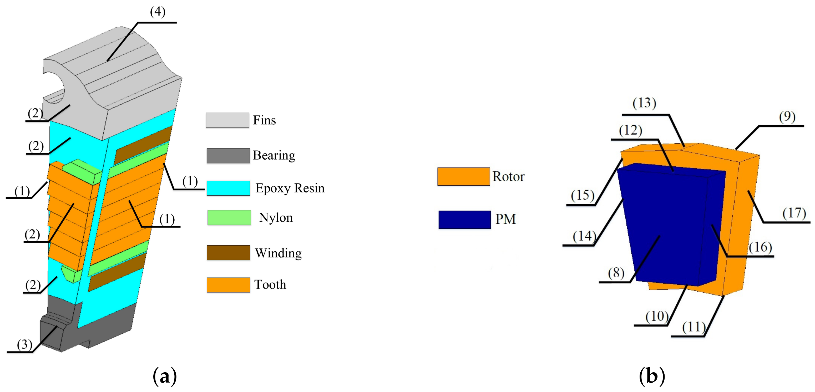
2. AFPMSM Lumped Parameter Thermal Modeling
2.1. YASA Machine Power Losses
2.1.1. Copper Losses
2.1.2. Core Losses
2.1.3. Permanent Magnet Losses
2.1.4. Mechanical Losses
2.2. Modeling of Convection Heat Transfer
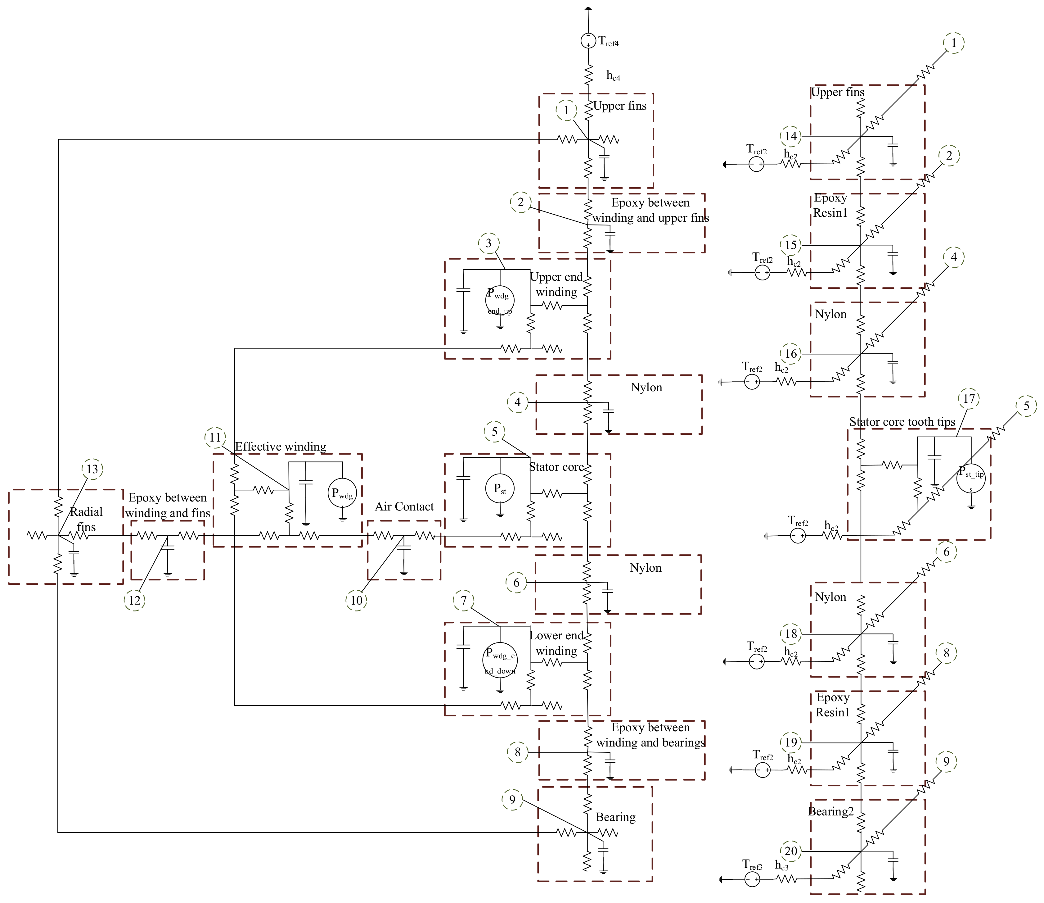
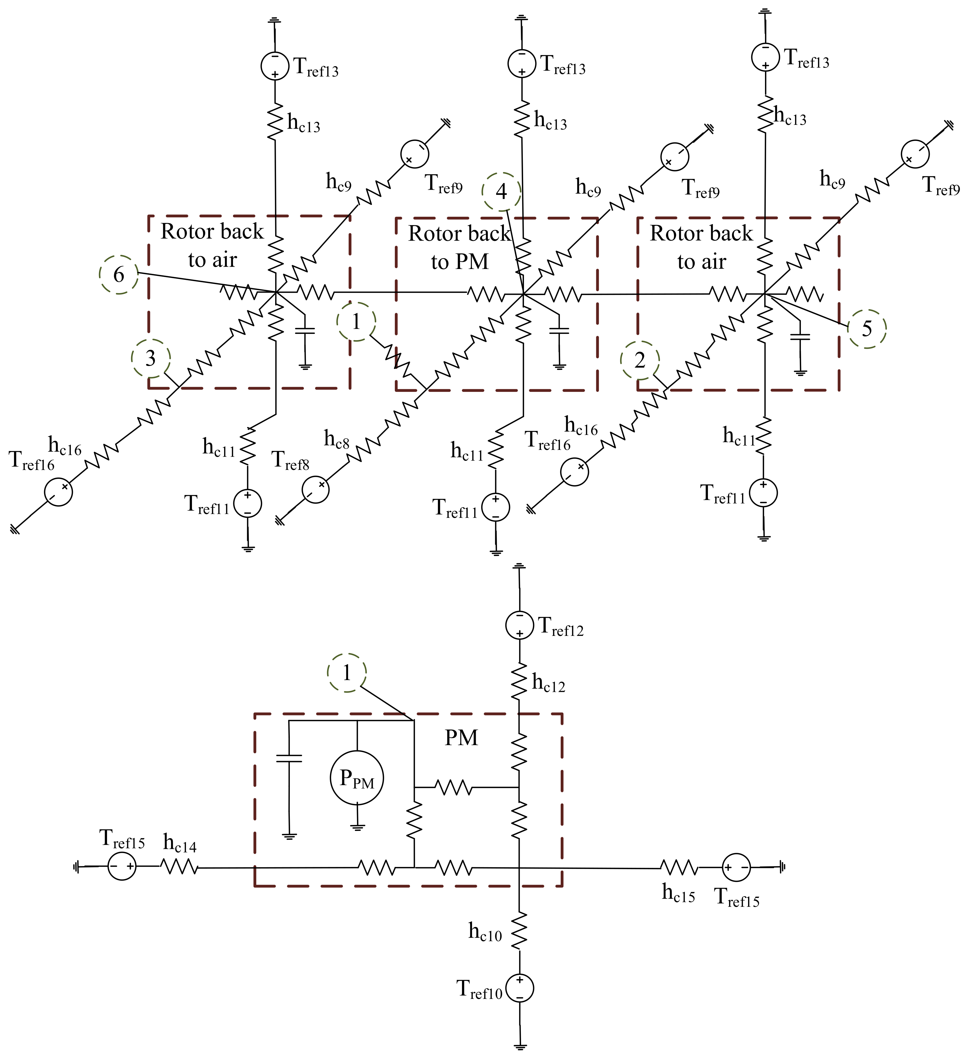
2.3. Lumped Parameter Thermal Network
2.4. Solution of the LPTN
3. 3D FEM Thermal Model
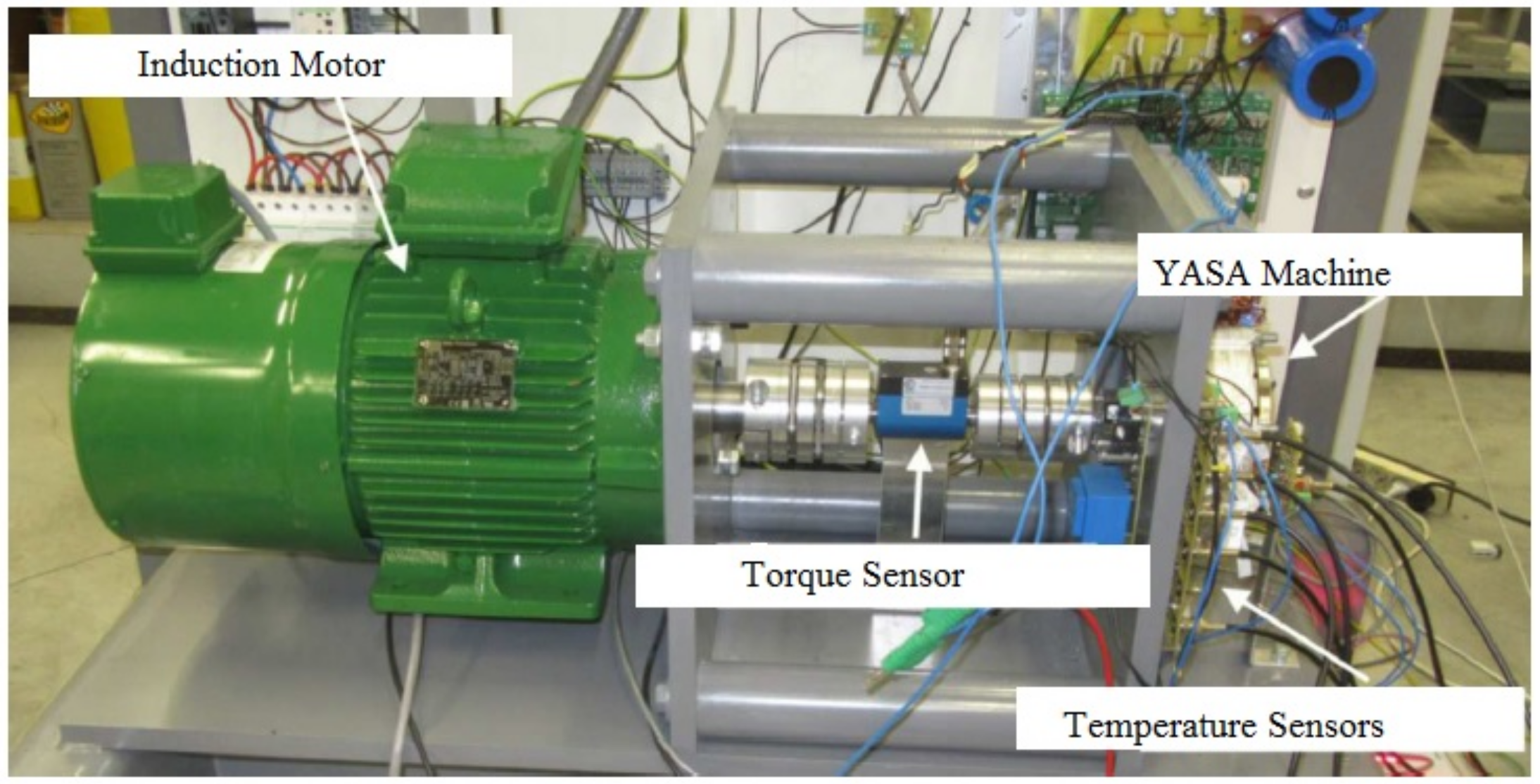
4. Experimental Setup and Results
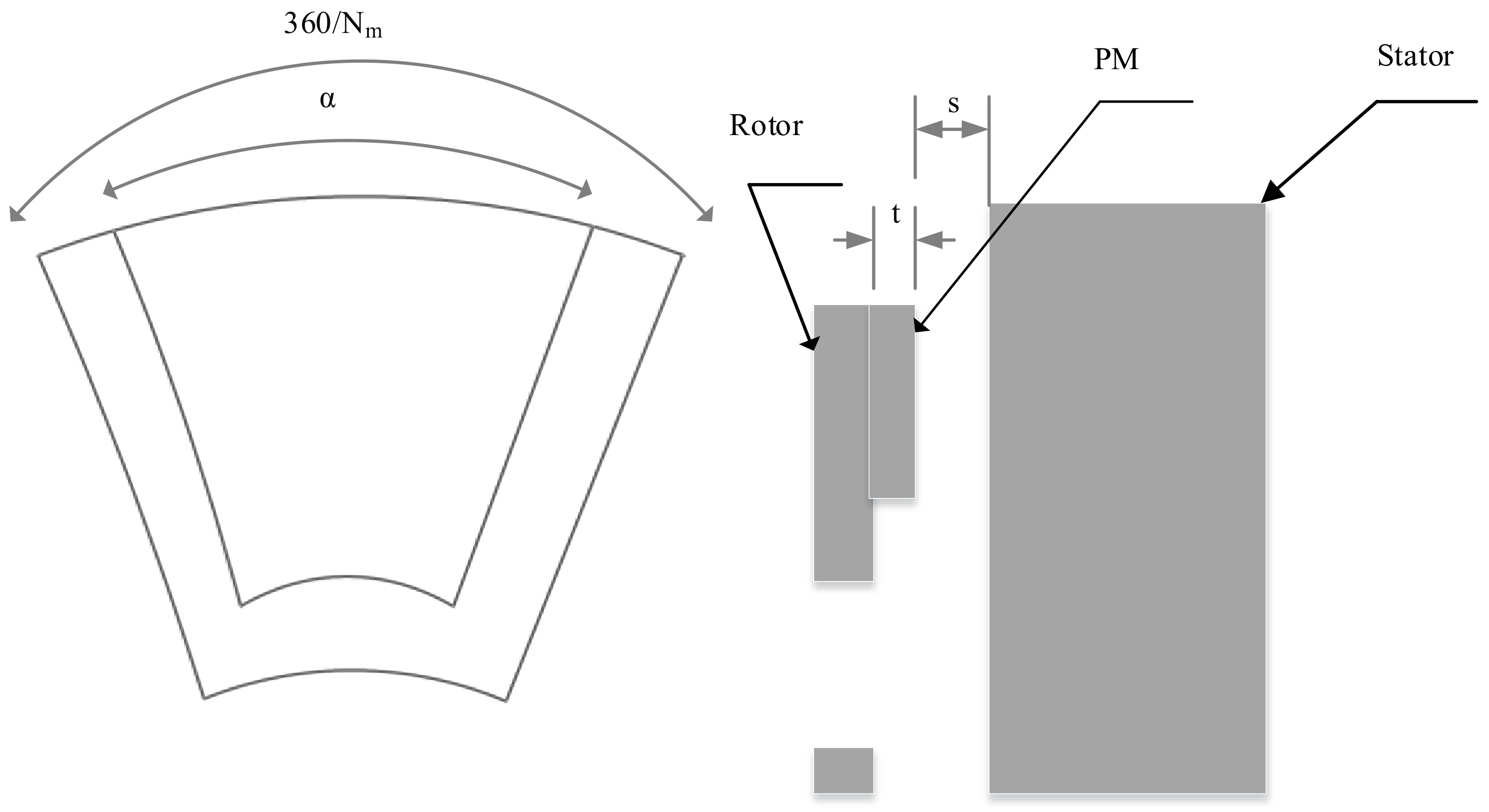
5. Model Validation at Different Parameters
5.1. Effect of
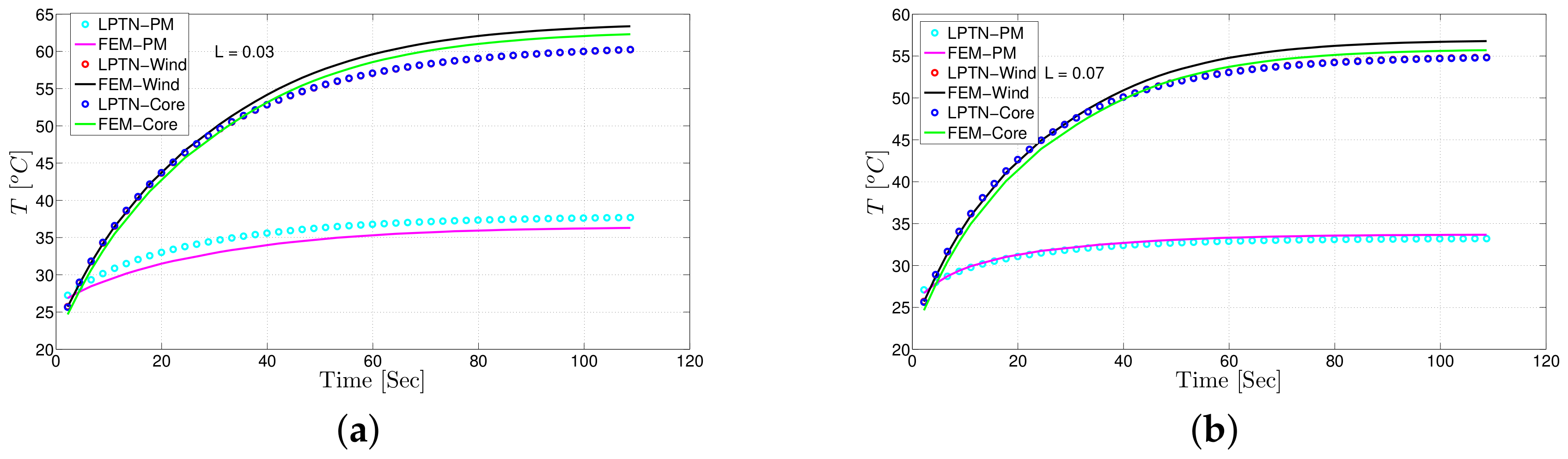
5.2. Effect of L
5.3. Effect of G
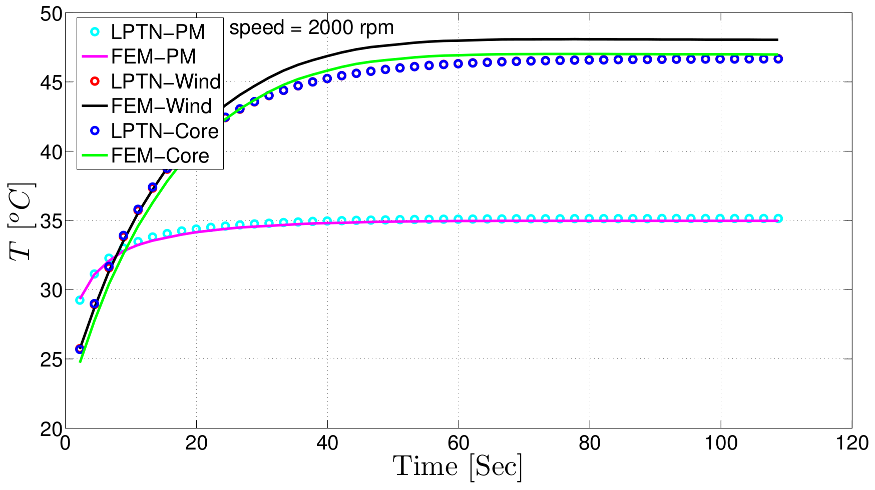
5.4. Effect of Rotor Speed
6. Conclusions
Acknowledgments
Author Contributions
Conflicts of Interest
References
- Du-Bar, C. Design of an Axial Flux Machine for an in-Wheel Motor Application; Chalmers Reproservice: Göteborg, Sweden, 2011. [Google Scholar]
- Tiegna, H.; Bellara, A.; Amara, Y.; Barakat, G. Analytical modeling of the open-circuit magnetic field in axial flux permanent-magnet machines with semi-closed slots. IEEE Trans. Magn. 2012, 48, 1212–1226. [Google Scholar] [CrossRef]
- Vansompel, H.; Sergeant, P.; Dupré, L. A multilayer 2-D-2-D coupled model for eddy current calculation in the rotor of an axial-flux PM machine. IEEE Trans. Energy Convers. 2012, 27, 784–791. [Google Scholar] [CrossRef]
- Hemeida, A.; Sergeant, P. Analytical modeling of surface PMSM using a combined solution of Maxwell’s equations and Magnetic Equivalent Circuit (MEC). IEEE Trans. Magn. 2014, 50, 7027913. [Google Scholar] [CrossRef]
- Hemeida, A.; Sergeant, P. Analytical modeling of eddy current losses in Axial Flux PMSM using resistance network. In Proceedings of the 2014 International Conference on Electrical Machines (ICEM), Berlin, Germany, 2–5 September 2014; pp. 2688–2694. [Google Scholar]
- Hemeida, A.; Sergeant, P.; Vansompel, H. Comparison of Methods for Permanent Magnet Eddy Current Loss Computations With and Without Reaction Field Considerations in Axial Flux PMSM. IEEE Trans. Magn. 2015, 9464. [Google Scholar] [CrossRef]
- Hemeida, A.; Hannon, B.; Sergeant, P. Comparison of three analytical methods for the precise calculation of cogging torque and torque ripple in PM machines. Math. Probl. Eng. 2016, 2016, 2171547. [Google Scholar] [CrossRef]
- Mueller, M.; McDonald, A.; Macpherson, D. Structural analysis of low-speed axial-flux permanent-magnet machines. IEE Proc. Electr. Power Appl. 2005, 152, 1417. [Google Scholar] [CrossRef]
- Vun, S.T.; McCulloch, M.D. Optimal Design Method for Large-Scale YASA Machines. IEEE Trans. Energy Convers. 2015, 30, 900–907. [Google Scholar] [CrossRef]
- Kumar, S.; Lipo, T.A.; Kwon, B.I. A 32000 r/min Axial Flux Permanent Magnet Machine for Energy Storage With Mechanical Stress Analysis. IEEE Trans. Magn. 2016, 52. [Google Scholar] [CrossRef]
- Hemeida, A.; Taha, M.; Abdallh, A.; Vansompel, H.; Dupré, L.; Sergeant, P. Applicability of Fractional Slot Axial Flux Permanent Magnet Synchronous Machines in the Field Weakening Region. IEEE Trans. Energy Convers. 2016, 32, 111–121. [Google Scholar] [CrossRef]
- Jiang, W.; Member, S.; Jahns, T.M. Coupled Electromagnetic—Thermal Analysis of Electric Machines Including Transient Operation Based on Finite-Element Techniques. In Proceedings of the 2013 IEEE Energy Conversion Congress and Exposition (ECCE), Denver, CO, USA, 15–19 September 2013; pp. 1880–1889. [Google Scholar]
- Tan, Z.; Song, X.G.; Ji, B.; Liu, Z.; Ma, J.E.; Cao, W.P. 3D thermal analysis of a permanent magnet motor with cooling fans. J. Zhejiang Univ. Sci. A 2015, 16, 616–621. [Google Scholar] [CrossRef]
- Polikarpova, M.; Ponomarev, P.; Lindh, P.; Petrov, I.; Jara, W.; Naumanen, V.; Tapia, J.A.; Pyrhonen, J. Hybrid Cooling Method of Axial-Flux Permanent-Magnet Machines for Vehicle Applications. IEEE Trans. Ind. Electron. 2015, 62, 7382–7390. [Google Scholar] [CrossRef]
- Marignetti, F.; Delli Colli, V.; Coia, Y. Design of Axial Flux PM Synchronous Machines Through 3-D Coupled Electromagnetic Thermal and Fluid-Dynamical Finite-Element Analysis. IEEE Trans. Ind. Electron. 2008, 55, 3591–3601. [Google Scholar] [CrossRef]
- Marignetti, F.; Colli, V. Thermal Analysis of an Axial Flux Permanent-Magnet Synchronous Machine. IEEE Trans. Magn. 2009, 45, 2970–2975. [Google Scholar] [CrossRef]
- Howey, D.A.; Holmes, A.S.; Pullen, K.R. Measurement and CFD Prediction of Heat Transfer in Air-Cooled Disc-Type Electrical Machines. IEEE Trans. Ind. Appl. 2011, 47, 1716–1723. [Google Scholar] [CrossRef]
- Rasekh, A.; Sergeant, P.; Vierendeels, J. Convective heat transfer prediction in disk-type electrical machines. Appl. Therm. Eng. 2015, 91, 778–790. [Google Scholar] [CrossRef]
- Rasekh, A.; Sergeant, P.; Vierendeels, J. Fully predictive heat transfer coefficient modeling of an axial flux permanent magnet synchronous machine with geometrical parameters of the magnets. Appl. Therm. Eng. 2017, 110, 1343–1357. [Google Scholar] [CrossRef]
- Sahin, F. Design and Development of a High-Speed Axial-Flux Permanent-Magnet Machine Design and Development of a High-Speed Axial-Flux Permanent-Magnet Machine. In Proceedings of the Conference Record of the 2001 IEEE Thirty-Sixth IAS Annual Meeting, Industry Applications Conference, Chicago, IL, USA, 30 September–4 October 2001. [Google Scholar]
- Vansompel, H.; Rasekh, A.; Hemeida, A.; Vierendeels, J.; Sergeant, P. Coupled Electromagnetic and Thermal Analysis of an Axial Flux PM Machine. IEEE Trans. Magn. 2015, 51. [Google Scholar] [CrossRef]
- Rostami, N.; Feyzi, M.R.; Pyrhonen, J.; Parviainen, A.; Niemela, M. Lumped-Parameter Thermal Model for Axial Flux Permanent Magnet Machines. IEEE Trans. Magn. 2013, 49, 1178–1184. [Google Scholar] [CrossRef]
- Lim, C.; Bumby, J.; Dominy, R.; Ingram, G.; Mahkamov, K.; Brown, N.; Mebarki, A.; Shanel, M. 2-D lumped-parameter thermal modelling of axial flux permanent magnet generators. In Proceedings of the 18th International Conference on Electrical Machines (ICEM 2008), Vilamoura, Portugal, 6–9 September 2008; pp. 1–6. [Google Scholar]
- Rasekh, A.; Sergeant, P.; Vierendeels, J. Development of correlations for windage power losses modeling in an axial flux permanent magnet synchronous machine with geometrical features of the magnets. Energies 2016, 9, 1009. [Google Scholar] [CrossRef]
- Mellor, P.; Roberts, D.; Turner, D. Lumped parameter thermal model for electrical machines of TEFC design. IEE Proc. B Electr. Power Appl. 1991, 138, 205–218. [Google Scholar] [CrossRef]
- Kuehbacher, D.; Kelleter, A.; Gerling, D. An improved approach for transient thermal modeling using lumped parameter networks. In Proceedings of the 2013 IEEE International Electric Machines & Drives Conference (IEMDC), Chicago, IL, USA, 12–15 May 2013; pp. 824–831. [Google Scholar]
- Kylander, G. Thermal Modelling of Small Cage Induction Motors. Ph.D. Thesis, School of Electrical and Computer Engineering, Chalmers University of Technology, Göteborg, Sweden, 1995. [Google Scholar]


| Material | K (W/mK) | (J/kgK) | (kg/m) |
|---|---|---|---|
| copper | 385 | 392 | 8890 |
| aluminum | 167 | 896 | 2712 |
| epoxy | 0.4 | 600 | 1540 |
| nylon | 0.25 | 1600 | 1140 |
| Nd-Fe-B | 9 | 500 | 7500 |
| Parameter | Value | Unit |
|---|---|---|
| number of poles | 16 | - |
| teeth number | 15 | - |
| outer diameter housing | 195 | mm |
| outer diameter active | 148 | mm |
| PM thickness | 4 | mm |
| rotor outer radius | 74 | mm |
| slot width | 11 | mm |
| Parameter | Value | Unit |
|---|---|---|
| air gap size ratio (G) | 0.0135 | - |
| PM thickness ratio (L) | 0.054 | - |
| PM angle ratio () | 0.8 | - |
| rotor speed | 1000 | rpm |
| Experimental | FEM | LPTN | % | % | |
|---|---|---|---|---|---|
| 56.029 | 56.529 | 56.529 | 0.9 | 0.9 | |
| 56.68 | 57.38 | 56.68 | 0 | 1.23 | |
| 35.582 | 35.18 | 34.782 | −2.24 | −1.12 |
© 2018 by the authors. Licensee MDPI, Basel, Switzerland. This article is an open access article distributed under the terms and conditions of the Creative Commons Attribution (CC BY) license (http://creativecommons.org/licenses/by/4.0/).
Share and Cite
Mohamed, A.H.; Hemeida, A.; Rasekh, A.; Vansompel, H.; Arkkio, A.; Sergeant, P. A 3D Dynamic Lumped Parameter Thermal Network of Air-Cooled YASA Axial Flux Permanent Magnet Synchronous Machine. Energies 2018, 11, 774. https://doi.org/10.3390/en11040774
Mohamed AH, Hemeida A, Rasekh A, Vansompel H, Arkkio A, Sergeant P. A 3D Dynamic Lumped Parameter Thermal Network of Air-Cooled YASA Axial Flux Permanent Magnet Synchronous Machine. Energies. 2018; 11(4):774. https://doi.org/10.3390/en11040774
Chicago/Turabian StyleMohamed, Abdalla Hussein, Ahmed Hemeida, Alireza Rasekh, Hendrik Vansompel, Antero Arkkio, and Peter Sergeant. 2018. "A 3D Dynamic Lumped Parameter Thermal Network of Air-Cooled YASA Axial Flux Permanent Magnet Synchronous Machine" Energies 11, no. 4: 774. https://doi.org/10.3390/en11040774