Location of Faulty Section and Faults in Hybrid Multi-Terminal Lines Based on Traveling Wave Methods

Abstract

Traveling-wave-based fault location methods are widely used for modern power systems owing to their high accuracy on two-terminal lines. However, they perform poorly on hybrid multi-terminal lines. Many traveling-wave-based methods have been developed recently to solve this problem, but they have high computational burdens and complex fault location procedures. To tackle this challenge, a new fault location method is presented in this paper. First, to ensure that the implementation of the proposed method is not affected by different line parameters, a normalization algorithm is used for hybrid multi-terminal lines, which consist of overhead lines and cables. To reduce the complexity, a novel fault section identification method that depends only on the first three arrival times is applied to separate a three-terminal fault section from the multi-terminal lines. Consequently, the fault can be located using a corresponding two-terminal fault location method in this fault section. To verify its effectiveness, fault case studies and performance evaluations are performed in the PSCAD and MATLAB/Simulink environment. The simulation results reveal that the proposed method can correctly identify the fault section and accurately locate the faults, which is simple and suitable for hybrid multi-terminal lines.

1. Introduction

Fault location is very important for quick system restoration and reducing economic loss in modern power systems. In recently years, the increased penetration of distributed generations (DGs) such as offshore wind farms (OWFs) and seashore wave power farms (SWPFs), has led to voltage imbalance and large ground current, resulting in permanent faults [1]. Furthermore, OWFs often connect with the main grid via hybrid multi-terminal lines. Hence, it is important to study fault location techniques for multi-terminal lines. Fault location methods have been widely studied and have achieved satisfactory performance in two-terminal transmission lines [2,3,4]. However, with respect to hybrid multi-terminal lines consisting of overhead lines and cables, accurate fault location is still a difficult task and needs more attention.

Common fault location methods can be divided into three categories: impedance-based methods [5], traveling-wave-based methods [6,7] and methods based on artificial intelligence algorithms [8]. Currently, impedance-based methods are the predominate method for transmission line fault location [9]. With the development of synchronized phasor measurements (PMUs), fault location techniques based on fundamental power frequency components have become promising [10,11]. In a multi-bus topology of power system, fault points can be located with minimal PMU placement [11]. In [12,13,14], the impedance matrix models for unbalanced three-phase line is described to analyse ground fault current and also to handle unsymmetrical faults with hybrid compensation for microgrid distribution systems. However, there are major errors in impedance-based fault location, mainly caused by fault resistance, line asymmetry, capacitive effect, or current transformer saturation [15]. Thus, traveling-wave-based methods have been widely used to avoid these drawbacks. The traveling-wave fault location methods based on transient-state analysis are more accurate than the impedance-based methods, because the accuracy of the former depends mainly on the sampling rates of the data acquisition system [16]. With the application of high-frequency transient recorders (TRs), traveling-wave methods have become more widely used in practice [17]. Different fault detection methods and their impact are reviewed in terms of protection performance in [18]. Wavelet transform has proved to be the best option for fault detection. In the traveling-wave methods, discrete wavelet transformation (DWT) is also frequently used to extract fault-induced transient signals. Artificial intelligence-based methods are often used for fault classification [8] and fault section identification. Combined with the relays and protection, an application of enhanced honey-bee mating optimization is proposed to solve the fault section estimation in [19].

Among the traveling-wave-based methods, the classical one-terminal method requires the identification of the traveling wave from the fault point [20], which is difficult to perform, particularly for multi-terminal lines. In [21], a classical two-terminal fault location method is presented where the measurement of traveling-wave arrival times needs to be synchronized. In [22], the use of ground and aerial mode traveling waves to determine the fault location is presented, and it is independent of the data synchronization and propagation velocity. In [23], the two-terminal method combined with support vector machines (SVM) is proposed for three-terminal overhead lines. However, the aforementioned traveling-wave methods often perform poorly in locating faults in multi-terminal networks.

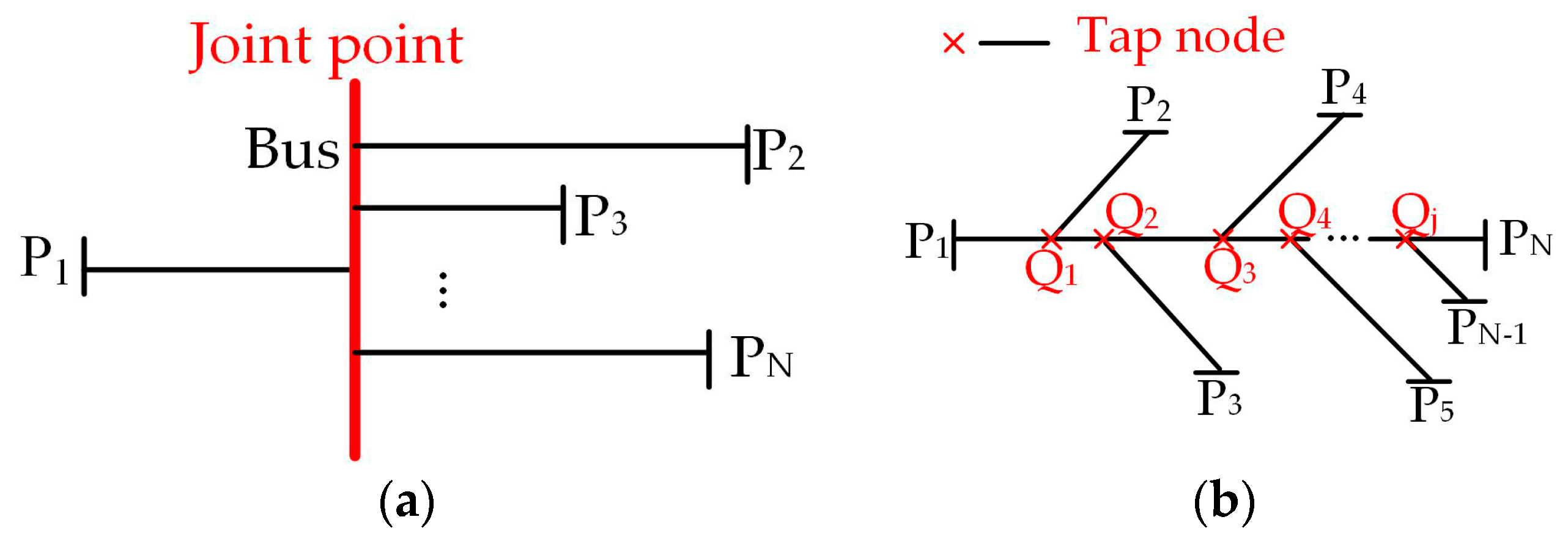
As structures have become complex in power transmission systems, in order to attain some kind of wide area protection, PMUs and traveling wave theory have been used to estimate a faulty area rather than for detection of exact fault points [24]. Therefore, research into accurate fault location detection methods within the faulty area is essential. Additionally, mesh line structures and radial line structures are widespread. In multi-terminal DC grids, aimed at mesh structures, the faulty segments are determined and accurate fault distance is then calculated based on the traveling wave method presented in [25]. Figure 1 shows two typical multi-terminal radial structures. In [26,27], using the matrix form of arrival time differences, the traveling-wave-based faulty line identification algorithm and fault-location formulation are applicable to the network in Figure 1a. However, the use of these methods is limited to the network in Figure 1b because the branches have no common joint point. To solve the fault location problems on the line structure in Figure 1b, several methods have been studied [28,29,30]. In [28], the identification and isolation of faulty sections depend on detecting the status of switch devices. In [29], the fault distance ratio matrix and rules to identify fault sections are proposed based on traveling waves. A multi-terminal technique to locate faults directly on branched networks has also been described [30], but these techniques have issues due to the high computational burden in the overhead line. Fault location problems become more complicated in multi-terminal hybrid transmission lines, especially for hybrid lines with overhead lines and cables, where the discontinuities in the wave impedance at the joint node need to be considered. According to [31], the implementation of fault location methods is restricted because the fault loop impedance does not linearly depend on the fault location, and additional reflections are created at the joint node. Moreover, the velocity of the traveling wave, which is an important propagation parameter, varies in lines and cables. The frequency characteristic of the traveling wave is more evident in cables. Therefore, in [32], support vector machine (SVM) classifiers are used to identify the fault section and faulty half of a two-terminal hybrid transmission line. However, this fault section identification method for hybrid lines has problems in multi-terminal line structures, as shown in Figure 1b.

Figure 1. Structure diagram of the multi-terminal radial lines: type (a) and type (b).

The proposed method eliminates the discontinuities of the wave velocity for hybrid multi-terminal lines, thus, the implementation of the following fault section identification and fault location method is not affected by the hybrid line parameters. Its most important advantage is that the first three measured arrival times are sufficient and can be directly used to divide a three-terminal fault section from multi-terminal lines. Identification of the fault section and fault location does not require many matrix calculations, which is simple and suitable for all multi-terminal structures compared to previous methods. Finally, the effectiveness of the proposed method is evaluated by the simulation results under different fault cases.

2. Overview of Traveling Wave Methods

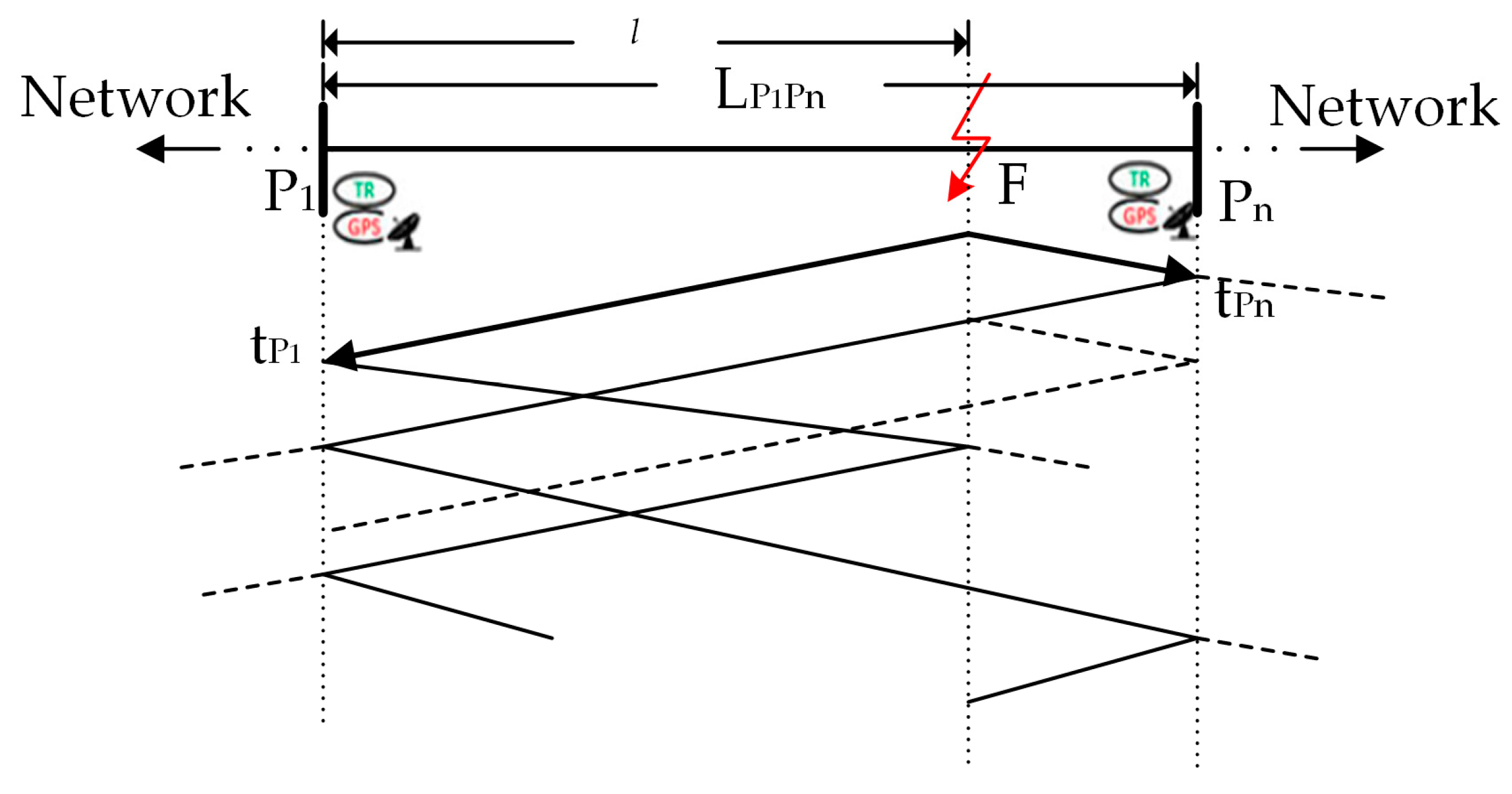
One- and two-terminal traveling wave methods use the traveling wave initiated by the fault or reflection characteristics on the lines [33,34]. When a fault occurs at an arbitrary position in the network, the traveling waves originated at the fault point will travel along both directions of the transmission line. To illustrate the traveling-wave-based method, Figure 2 depicts the propagation pattern of fault-induced traveling waves, where TRs [27] are installed at terminal P₁ and P_n, the first traveling waves reach P₁ and P_n at instants t_P1 and t_Pn, L_P1Pn is the line length between P₁ and P_n. The two-terminal method is more reliable because only the first traveling waves need to be detected. Base on the two-terminal method, the calculated fault distance from measuring point P₁ is obtained as follows:

$$l_{\mathrm{CFD}}=L_{{\mathrm{P}}_1\mathrm{F}}=\frac{v(t_{{\mathrm{P}}_1}-t_{{\mathrm{P}}_{\mathrm{n}}})+L_{{\mathrm{P}}_1{\mathrm{P}}_{\mathrm{n}}}}{2}$$

(1)

where v is the traveling-wave propagation velocity. It should be noted that v is different in overhead lines and cables. Therefore, Equation (1) cannot be applied directly in hybrid lines because of the discontinuity of the propagation velocity.

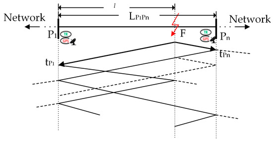
Figure 2. Propagation of fault-induced traveling waves.

In multi-terminal lines, the propagation of reflected and refracted traveling waves is more complicated because the propagation shown in Figure 2 exists between any two terminals. In Figure 3, a multi-terminal line monitored at two terminals is taken as an analysis model.

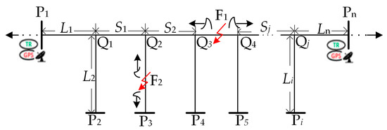
Figure 3. Multi-terminal line model monitored at two terminals.

To provide a better understanding of the description and analysis below, all nodes are divided into two groups: terminal nodes P_i and tap nodes Q_j (i and j = 1, 2, …, n). L_PiQj is the length between two nodes, the length between two tap nodes is recorded as S_j, and the length of a branch is recorded as L_i. The line between two terminals equipped with TRs is defined as the main line. If the fault occurs in the main line, the fault distance is the same as Equation (1). If the fault is in the branch which connect the main line at node Q₂, the following equations apply:

$$\{\begin{array}{l}{L}_{{\mathrm{P}}_1\mathrm{F}}-L_{{\mathrm{P}}_{\mathrm{n}}\mathrm{F}}=v(t_{{\mathrm{P}}_1}-t_0)-v(t_{{\mathrm{P}}_{\mathrm{n}}}-t_0)\\ L_{{\mathrm{P}}_1{\mathrm{Q}}_2}+L_{{\mathrm{P}}_{\mathrm{n}}{\mathrm{Q}}_2}=L_{{\mathrm{P}}_1{\mathrm{P}}_{\mathrm{n}}}\\ L_{{\mathrm{P}}_1{\mathrm{Q}}_2}+L_{{\mathrm{Q}}_2\mathrm{F}}=L_{{\mathrm{P}}_1\mathrm{F}}\\ L_{{\mathrm{P}}_{\mathrm{n}}{\mathrm{Q}}_2}+L_{{\mathrm{Q}}_2\mathrm{F}}=L_{{\mathrm{P}}_{\mathrm{n}}\mathrm{F}}\end{array}$$

(2)

$$l_{\mathrm{CFD}}=L_{{\mathrm{P}}_1{\mathrm{Q}}_2}=\frac{v(t_{{\mathrm{P}}_1}-t_{{\mathrm{P}}_{\mathrm{n}}})+L_{{\mathrm{P}}_1{\mathrm{P}}_{\mathrm{n}}}}{2}$$

(3)

where the time of initialization of the fault is recorded as t₀. v is the traveling-wave propagation velocity. Equations (1) and (3) are calculated using the two-terminal-based method, but the results of the calculation are different. For the fault in the main line, Equation (1) calculates the actual fault distance, but if the fault occurs in the branch, Equation (3) calculates the distance between the measurement point and the tap node. Thus, the two-terminal-based method fails to identify faults in branches. Two-terminal measurement data are insufficient to detect the fault point in multi-terminal lines.

To solve this problem, TRs are installed at all terminals and the synchronized transient signals at each terminal are generally used for fault location [27]. However, the existing method builds a 3-D ratio matrix, which contains the difference in distance between any two terminals at any point in the network [30]. In particular, for large networks, major issues related to complex modeling and computational burden can be avoided in this application. In this paper, the proposed method identifies the fault sections and locates fault points with less calculation than previous methods.

3. Proposed Fault Location Method for Hybrid Multi-Terminal Lines

The proposed method is based on the following preconditions: The line segment or branch is not significantly longer than others in modern power networks. All terminals are equipped with global position system (GPS) signal receivers to synchronize the TRs. The coupling capacitor voltage transformer (CCVT) has been proven to have a good performance in transient voltage measurement [35]. The path lengths that the traveling wave passed along are known in advance.

Figure 4 presents the overall flowchart of the proposed method. After a normalization algorithm for the hybrid multi-terminal line, the core idea of this paper was to identify the fault section using the first three arrival times and implement the corresponding fault location procedure. Among these steps, the arrival time extraction uses a general method, which is similar to other references [36,37]. Generally, wavelet transform is a well-known and powerful tool to detect transients in power systems, which is also applied to extract the arrival times of traveling waves in this paper. The transient voltages are measured using TRs and then transformed into the modal domain using Clarke transformation. A discrete wavelet transformation (DWT) is applied to extract the aerial mode voltage, and the first arrival times of the traveling wave are obtained by marking the squares of wavelet transformation coefficients (WTC²s). The other steps including normalization algorithm, fault section identification and fault location are presented below.

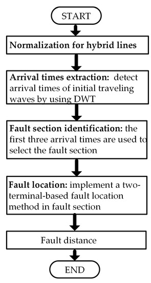
Figure 4. Overall flowchart of the proposed method.

3.1. Normalization Algrithms

For hybrid multi-terminal lines, the propagation velocity of the traveling wave is obviously different in overhead lines and cables. The propagation velocity, as one of the important parameters is properly estimated in the traveling wave method. Generally, the actual velocity v in the overhead line is approximately 98% of the speed of light. According to [38], the propagation velocity in the cables is an a priori value and is approximately one-third to one-half of the speed of light. Therefore, classical traveling wave methods cannot be directly used in hybrid multi-terminal lines. The discontinuity of the traveling-wave velocity at the joint point must be eliminated. To solve this problem, a normalization algorithm is used in this paper. All cables are equivalent to overhead lines through Equation (4) as follows:

$$L_{\mathrm{eq}}=L_{\mathrm{cable}}\times v/v_{\mathrm{cable}}$$

(4)

where L_eq and L_cable are the equivalent length and actual length of cable segments, respectively. v and v_cable are the corresponding propagation velocities in the overhead lines and cables, respectively. The propagation velocity under a certain frequency can be calculated from the line parameters. After the proposed normalization algorithm, the hybrid multi-terminal lines consist of the original overhead lines and new overhead lines with equivalent lengths. In this condition, the fault section identification and fault location method can be designed without considering the hybrid structure.

3.2. Fault Section Identification

When a fault occurs on the transmission line, the fault-induced traveling wave propagates in both directions from the fault point. The arrival time t_Pi, travel distance s, and velocity v are related as follows:

$$t_{{\mathrm{p}}_i}=t_0+s/v$$

(5)

The arrival time t_Pi is linearly proportional to the travel distance s. The traveling wave arrival times detected at each terminal are sorted according to the sequence of arrival times, the first three are recorded as t_first, t_second and t_third, and the corresponding travel distances are recorded as s_first, s_second and s_third. The relationship of arrival times is t_first < t_second < t_third; according to (5), the relationship of travel distances is s_first < s_second < s_third.

Using the first three arrival times, a possible three-terminal fault network can be obtained. Different fault positions (fault in the branch and fault between two tap nodes) are considered to prove that the fault is located in this three-terminal network. According to the propagation of traveling waves, two types of situations are considered: situation I, the first three times are detected from one direction; and situation II, the first three times are detected from both directions.

Figure 5 shows situation I, the terminals P_f, P_s, and P_t are defined as the receiving points for traveling waves, where the first three arrival times are detected. These three receiving points constitute a three-terminal section enclosed by dotted line. No matter if a fault point F is in a branch or between two nodes, it is outside of the three-terminal section. If this situation can be proved not to happen, it is certain that the fault will locate in the three-terminal section. Then the analysis process is as follows. In this situation, for the fault in the branch in Figure 5a, according to s_first < s_second < s_third, the travel distance satisfies the relationship: (1 − λ)L₁ + L₂<(1 − λ)L₁ + S₁ + L₃ < (1 − λ)L₁ + S₁ + S₂ + L₄, where λ is the ratio of the fault distance to the faulty line length. S₁, S₂, L₄, and L₁ are the lengths of the lines. If the first three traveling waves propagate along one direction, the precondition s_third < λL₁ must be satisfied as follows:

$$\left(1-\lambda \right)L_1+S_1+S_2+L_4<\lambda L_1$$

(6)

Figure 5. Situation of the first three arrival times detected from one direction. (a) Fault in a branch. (b) Fault in main line between two tap nodes.

Then, (6) can be rewritten as

$$\frac{1}{2}(1+\frac{S_1+S_2+L_4}{L_1})<\lambda$$

(7)

since 0 < λ < 1, (7) can be described as

$$\frac{1}{2}(1+\frac{S_1+S_2+L_4}{L_1})<0$$

(8)

From (7), (8) can be obtained as follows:

$$\frac{S_1+S_2+L_4}{L_1}<-1$$

(9)

where S₁, S₂, L₄, and L₁ are positive. Therefore, the result of (9) must be false. The fault situation in Figure 5a can be excluded. Similarly, for the fault between two tap nodes in Figure 5b, under the assumption for the first three arrival times, the corresponding travel distance should satisfy the relationship: (1 − λ)S₁ + L₃ < (1 − λ)S₁ + S₂ + L₄ < (1 − λ)S₁ + S₂ + S₃ + L₅. The precondition for the distance should satisfy s_third < min(L₁ + λS₁, L₂ + λS₁). Assuming that L₁ + λS₁ < L₂ + λS₁, from Figure 5b, that is given by

$$\left(1-\lambda \right)S_1+S_2+S_3+L_5<L_1+\lambda S_1$$

(10)

Then, by rewriting (10) like (7) and (8), we have

$$S_1+S_2+S_3+L_5<L_1$$

(11)

However, the configuration of the line length in (11) is not an optimized network structure and rarely appears in actual modern power systems. Thus, the fault situation in Figure 5b is not considered in this paper. Based on the above analysis, we conclude that the first three arrival times may not be detected from one direction, which means that the situation of faults outside of the three-terminal section is inexistent.

Figure 6 shows situation II, where the first three times are detected from both directions. From Figure 6, it can be seen that no matter where the fault is located, it is always in the three-terminal section. Furthermore, in this situation, neither the position of the fault nor the line length needs to be analyzed as in situation I. We also conclude that the fault is located in the three-terminal section.

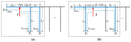
Figure 6. Situation of the first three arrival times detected from both direction. (a) Fault in a branch. (b) Fault in main line between two tap nodes.

According to the analysis of the two aforementioned types of situation, a fault section can be identified by the first three arrival times. A three-terminal section is separated from multi-terminal lines as the fault section, and the fault location procedure is implemented on this basis.

3.3. Fault Location

After the fault section is identified, the two-terminal traveling-wave-based method is used for fault location. Figure 7 shows the three-terminal fault section separated from the multi-terminal lines.

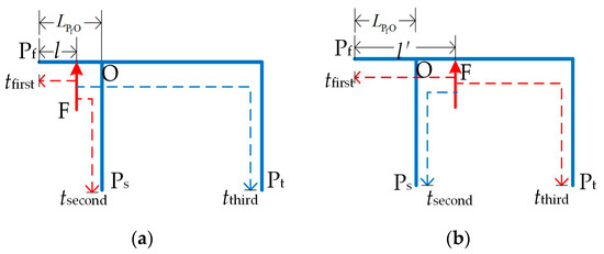
Figure 7. Three-terminal fault section separated from the multi-terminal lines. (a) Fault between P_f and P_s. (b) Fault between P_f and P_t.

In Figure 7, the terminals where the first three arrival times are detected are P_f, P_s, and P_t. The tap node is recorded as O. Because the overhead line traveling-wave velocity and the line length between any two terminals are known, the distance of the fault to P_f is calculated using t_first and t_second as follows:

$$l=0.5\left[L_{{\mathrm{p}}_{\mathrm{f}}{\mathrm{p}}_{\mathrm{s}}}+v(t_{\mathrm{first}}-t_{\sec \mathrm{ond}})\right]$$

(12)

where the time difference between the first (t_first) and second (t_second) arrival times is used. Based on the description in Section 2, ideally, if the calculated distance is not equal to L_PfO, the fault distance should be l, as shown in Figure 7a. If the calculated distance is equal to L_PfO, the fault distance from P_f calculated using t_first and t_third is as follows:

$$l^{\prime }=0.5\left[L_{{\mathrm{p}}_{\mathrm{f}}{\mathrm{p}}_{\mathrm{t}}}+v(t_{\mathrm{first}}-t_{\mathrm{third}})\right]$$

(13)

where the time difference between the first (t_first) and the third (t_third) arrival times is used for fault location, as shown in Figure 7b. However, when considering the measurement error, 0.5%L_PfO is used as the marginal error. An absolute value Δ denotes the difference value between the fault point and the tap node, which is defined as:

$$\Delta =\left|l-L_{{\mathrm{P}}_{\mathrm{f}}\mathrm{O}}\right|$$

(14)

If Δ > 0.5%L_PfO, the fault distance is obtained by (12); if Δ < 0.5%L_PfO, the calculated fault distance is obtained by (13), which is given by

$$l_{\mathrm{CFD}}=\{\begin{array}{ll}l& \Delta >0.5\%L_{{\mathrm{P}}_{\mathrm{f}}\mathrm{O}}\\ l^{\prime }& \Delta <0.5\%L_{{\mathrm{P}}_{\mathrm{f}}\mathrm{O}}\end{array}$$

(15)

In addition, the aforementioned fault distance is obtained after the normalization algorithm for the hybrid multi-terminal lines. When the fault point is located in cables, the final fault distance must be further calculated as follows:

$$l^{*}=(l_{\mathrm{CFD}}-L_{\mathrm{overhead}-\mathrm{line}})\times v_{\mathrm{cable}}/v+L_{\mathrm{overhead}-\mathrm{line}}$$

(16)

where l* is the fault distance obtained by the inverse process of normalization. L_{overhead-line} is the overhead line length in fault distance.

4. Simulation Results

4.1. The Model of Simulation

To evaluate the proposed method, a nine-terminal 220-kV/50-Hz hybrid line simulation system (Figure 8) was developed in PSCAD (PSCADX4.5, Manitoba HVDC Research Centre Inc., Winnipeg, MB, Canada) and MATLAB/Simulink (R2016a, MathWorks, Natick, MA, USA). The post-fault analysis is performed using DWT with a 200-kHz sampling frequency. In the test network, nine TRs are positioned at the branch terminals and labeled P₁–P₉. The tap nodes are labeled Q₁–Q₇. The branch Q₄P₅, segments Q₂Q₃ and Q₅Q₇ are assumed to be cables, and the others are overhead lines. The line lengths of each branch and segment are shown in Figure 8. All overhead lines and cables are modeled with distributed parameters, which are provided in Table 1. The propagation velocities are v = 2.9242 × 10⁵ km/s in the overhead line and v_cable = 1.4813 × 10⁵ km/s in the cable.

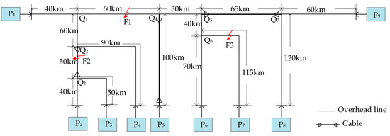
Figure 8. Nine-terminal hybrid line simulation system.

Table 1. Parameters of lines.

Type	Source	Impendence Z (Ω/km)	Admittance Y (S/km)
Overhead line	Zero source	0.362 + j1.1426	j1.936 × 10−6
	Positive source	0.035 + j0.4234	j2.726 × 10−6
Cable	Zero source	0.032 + j0.188	j44.367 × 10−6
	Positive source	0.028 + j0.072	j62.471 × 10−6

According to the normalization algorithm mentioned in Section 3, the equivalent lengths of cables are calculated and listed in Table 2.

Table 2. Normalization for cables.

Segment	Cable Length Lcable (km)	Equivalent Length Leq (km)
Q4P5	100	197.41
Q2Q3	50	98.70
Q5Q7	65	128.32

4.2. Typical Case Study of the Proposed Method

The processes of the proposed method for three typical cases are illustrated as follows. As a common practice, the relative error is used to assess the accuracy of the proposed fault location method [39]:

$$Error(\%)=\frac{\left|\mathrm{Calculated}\mathrm{fault}\mathrm{distance}-\mathrm{Actual}\mathrm{fault}\mathrm{distance}\right|}{\mathrm{total}\mathrm{length}\mathrm{of}\mathrm{fault}\sec \mathrm{tion}}$$

(17)

4.2.1. Test Case 1: AG Fault in Overhead Line Segment

The first case occurs on an overhead line segment (between two nodes Q₁ and Q₄), which is an A-phase-to-ground (AG) fault F1, 80 km from terminal P₁, and the fault resistance Z_f is 10 Ω. DWT is used for the aerial mode voltage at terminals P₁–P₉. The voltages WTC²s are shown in Figure 9, and the corresponding first arrival times are listed in Table 3. The first three arrival times are t_first = 10.295 ms, t_second = 10.570 ms and t_third = 10.670 ms, which are measured at terminals P₁, P₆ and P₄, respectively. According to the analysis in Section 3.2, the fault section is shown in Figure 10, which is a three-terminal network composed by the propagation path of the first three initial waves. After identification of the fault section, the proposed fault location method can be implemented. First, using Equation (12), the distance from P₁ (P_f) is calculated by

$$l=\frac{240+2.9242\times {10}^5\times (10.295-10.570)\times {10}^{-3}}{2}=79.792\mathrm{km}$$

(18)

where L_PfPs = 240 km and L_PfO = 130 km. According to the proposed fault location method, the marginal errors 0.5%L_PfO = 0.65 and Δ = 50.208 > 0.65 are calculated in this case. Thus, the fault distance is l_CFD = l, which is estimated using (15). Finally, according to (17), the error in this case is |79.792 − 80|/390 = 0.053%.

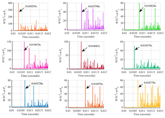
Figure 9. Arrival times at each terminal obtained by voltage WTC²s for AG fault F1.

Table 3. Arrival times of the initial traveling wave for fault F1 with fault initialization time = 0.01 s.

Terminal	Arrival Time (ms)	Terminal	Arrival Time (ms)	Terminal	Arrival Time (ms)
P1	10.295	P4	10.670	P7	10.720
P2	10.790	P5	10.685	P8	10.970
P3	10.820	P6	10.570	P9	10.770

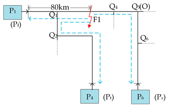
Figure 10. Identified three-terminal fault section for fault F1.

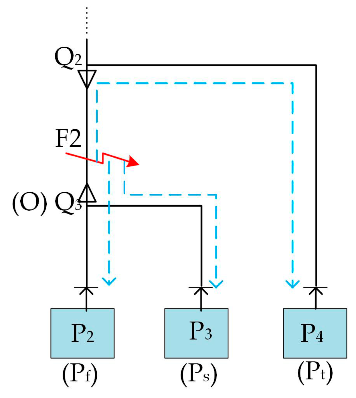
4.2.2. Test Case 2: ABG Fault in Cable Line Segment

In the second case, an AB-phase-to-ground (ABG) fault F2 occurs in cable segment Q₂Q₃ at 70 km from terminal P₂ with the fault resistance Z_f = 50 Ω. The arrival times of the initial traveling wave are listed in Table 4. The first arrival time is t_first = 10.360 ms measured at terminal P₂; the second arrival time is t_second = 10.395 ms measured at terminal P₃; and the third arrival time is t_third = 10.465 ms measured at terminal P₄. The fault section, which consists of the lines between P₂, P₃ and P₄, are shown in Figure 11. After identifying the fault section, the distance from P₂ (P_f) is calculated using (12) as

$$l=\frac{90+2.9242\times {10}^5\times (10.360-10.395)\times {10}^{-3}}{2}=39.883km$$

(19)

where L_PfPs = 90 km and L_PfO = 40 km. 0.5%L_PfO = 0.2 and Δ = 0.117 are calculated. Because Δ < 0.5%L_PfO, the fault distance is l_CFD = l′, which should be calculated using (13)

$$l^{\prime }=\frac{228.7+2.9242\times {10}^5\times (10.360-10.465)\times {10}^{-3}}{2} =98.998km$$

(20)

where the equivalent length is L_PfPt = 228.7 km. Since a cable (Q₂Q₃) is included in the three-terminal fault section, the actual distance is calculated using (16)

$$l^{*}=(98.998-40)\times \frac{1.4813}{2.9242}+40=69.886km$$

(21)

Table 4. Arrival times of the initial traveling wave for fault F2 with fault initialization time = 0.01 s.

Terminal	Arrival Time (ms)	Terminal	Arrival Time (ms)	Terminal	Arrival Time (ms)
P1	10.500	P4	10.465	P7	11.200
P2	10.360	P5	11.240	P8	11.520
P3	10.395	P6	11.045	P9	11.310

Figure 11. Identified three-terminal fault section for fault F2.

Finally, the error of this case is |70 − 69.886|/230 = 0.049%.

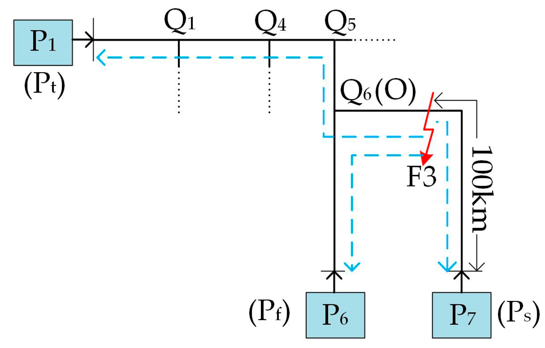
4.2.3. Test Case 3: AB Fault in Branch

The third case is a AB-phase-to-phase (AB) fault F3 in the overhead line branch Q₆P₇, which is 100 km from terminal P₇ with a fault resistance of Z_f = 100 Ω. The arrival times of the initial traveling wave are also listed in Table 5. The first three arrival times are t_first = 10.310 μs, t_second = 10.365 μs and t_third = 10.665 μs, and they are measured at terminals P₆, P₇ and P₁, respectively. The three-terminal fault section for F3 is shown in Figure 12. Firstly, the distance of the fault to terminal P₆ (P_f) is calculated using (12),

$$l=\frac{180+2.9242\times {10}^5\times (10.310-10.365)\times {10}^{-3}}{2}=84.458km$$

(22)

where L_PfPs = 185 km and L_PfO = 70 km. We calculate 0.5%L_PfO = 0.35 and Δ = 14.458. The relationship between the marginal error and the absolute error satisfies Δ > 0.5%L_PfO, the calculated distance l obtained from Equation (22) is the fault distance. However, to be consistent with the assumption in this case, the distance from the fault to terminal P₇ is obtained by L_PfPs−l = 185 − 84.458 = 100.542 km, and the error in this case is |100 − 100.542|/355 = 0.152%.

Table 5. Arrival times of the initial traveling wave for fault F3 with fault initialization time = 0.01 s.

Terminal	Arrival Time (ms)	Terminal	Arrival Time (ms)	Terminal	Arrival Time (ms)
P1	10.665	P4	11.030	P7	10.365
P2	11.195	P5	10.985	P8	11.060
P3	11.230	P6	10.310	P9	10.855

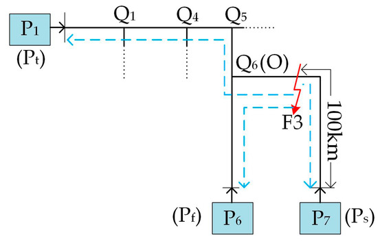
Figure 12. Identified three-terminal fault section for fault F3.

Furthermore, more fault points in each segment of the simulation system have been tested. The fault section identification and fault location results in different positions are included in Table 6. From Table 6, it can be seen that satisfactory results were obtained. These verify that the proposed method can be used to locate faulty section and fault point, no matter where the faults occur. The faulty section was correctly identified in 100% of cases, although the error is relatively large for a fault near terminals and tap nodes. Also, the location accuracy of the proposed method is not affected by the fault positions.

Table 6. Section identification and fault location results in different positions.

Segment	Fault Location	Fault Section	Actual FD from Pf (km)	Calculate FD (km)	Error (%)
		Pf Ps Pt
P1−Q1	10 km from P1	P1 P4 P6	10	10.198	0.051
Q1−Q2	15 km from Q1	P1 P4 P2	55	54.792	0.063
Q1−Q2	40 km from Q1	P1 P4 P2	80	79.648	0.107
Q2−Q3	5 km from Q2	P4 P1 P2	95	95.299	0.110
Q2−Q3	20 km from Q2	P2 P3 P4	70	69.886	0.049
Q3−P2	12 km from P2	P2 P3 P4	12	11.872	0.055
Q3−P3	34 km from P3	P3 P2 P4	34	34.034	0.015
Q2−P4	20 km from P4	P4 P1 P2	20	19.702	0.106
Q2−P4	80 km from P4	P4 P1 P2	80	79.648	0.126
Q1−Q4	40 km from Q1	P1 P6 P4	80	79.792	0.053
Q4−P5	37 km from P5	P5 P1 P6	37	36.815	0.054
Q4−P5	90 km from P5	P1 P6 P5	110	109.859	0.041
Q4−Q5	15 km from Q4	P1 P6 P7	115	115.614	0.173
Q5−Q6	20 km from Q5	P6 P7 P1	90	90.027	0.008
Q6−P6	45 km from P6	P6 P7 P1	45	44.982	0.005
Q6−P7	100 km from P7	P6 P7 P1	85	84.458	0.153
Q5−Q7	30 k m from Q5	P9 P6 P8	95	95.167	0.047
Q7−P8	100 k m from P8	P9 P8 P6	80	79.765	0.066
Q7−P9	30 km from P9	P9 P8 P6	30	30.054	0.015

4.3. Performance Evaluation

To validate the robustness of the proposed fault-location method, three fault cases with various fault inception angles (FIA), fault resistance (FR) and fault types are simulated, as shown in Table 7. We can see from this table, that the proposed method can find the fault location with satisfactory accuracy. The proposed method has strong tolerance for the FIA, FR and fault type. The impacts of these parameters is discussed below.

Table 7. Results of fault location for different conditions.

Fault	F-R (Ω)	FIA (°)	Relative Error (%)
			SLG	LLG	LL	3L/3LG
F1	10	90	0.053	0.053	0.052	0.051
		45	0.058	0.058	0.056	0.056
		10	0.063	0.063	0.062	0.062
	50	90	0.055	0.055	0.055	0.055
		45	0.060	0.058	0.058	0.060
		10	0.067	0.064	0.064	0.064
	100	90	0.057	0.057	0.056	0.056
		45	0.063	0.063	0.062	0.062
		10	0.074	0.074	0.072	0.072
F2	10	90	0.045	0.045	0.044	0.044
		45	0.049	0.049	0.047	0.048
		10	0.057	0.055	0.055	0.055
	50	90	0.049	0.048	0.049	0.048
		45	0.053	0.052	0.051	0.051
		10	0.061	0.059	0.059	0.057
	100	90	0.051	0.051	0.050	0.050
		45	0.063	0.061	0.061	0.061
		10	0.067	0.065	0.063	0.061
F3	10	90	0.143	0.143	0.143	0.143
		45	0.145	0.145	0.145	0.145
		10	0.154	0.154	0.153	0.154
	50	90	0.146	0.146	0.146	0.146
		45	0.150	0.150	0.148	0.148
		10	0.159	0.156	0.154	0.152
	100	90	0.152	0.150	0.148	0.148
		45	0.157	0.154	0.151	0.151
		10	0.163	0.161	0.157	0.157

In this paper, all fault types (i.e., single-line-to-ground (SLG), line-to-line-to-ground (LLG), line-to-line (LL), and three-phase faults (3L/3LG)) are discussed. It can be seen from all rows of Table 7, that all results are insensitive to different fault types. The errors are smallest for three-phase faults. This is because the initial waves become more detectable with the increase in the magnitude of traveling waves for multi-phase faults [27].

According to Table 7, it can be concluded that the fault location errors are minimal when FIA = 90°, when the fault resistance is constant. Although the relative location errors slightly vary with fault inception angles, the location accuracy can still be guaranteed.

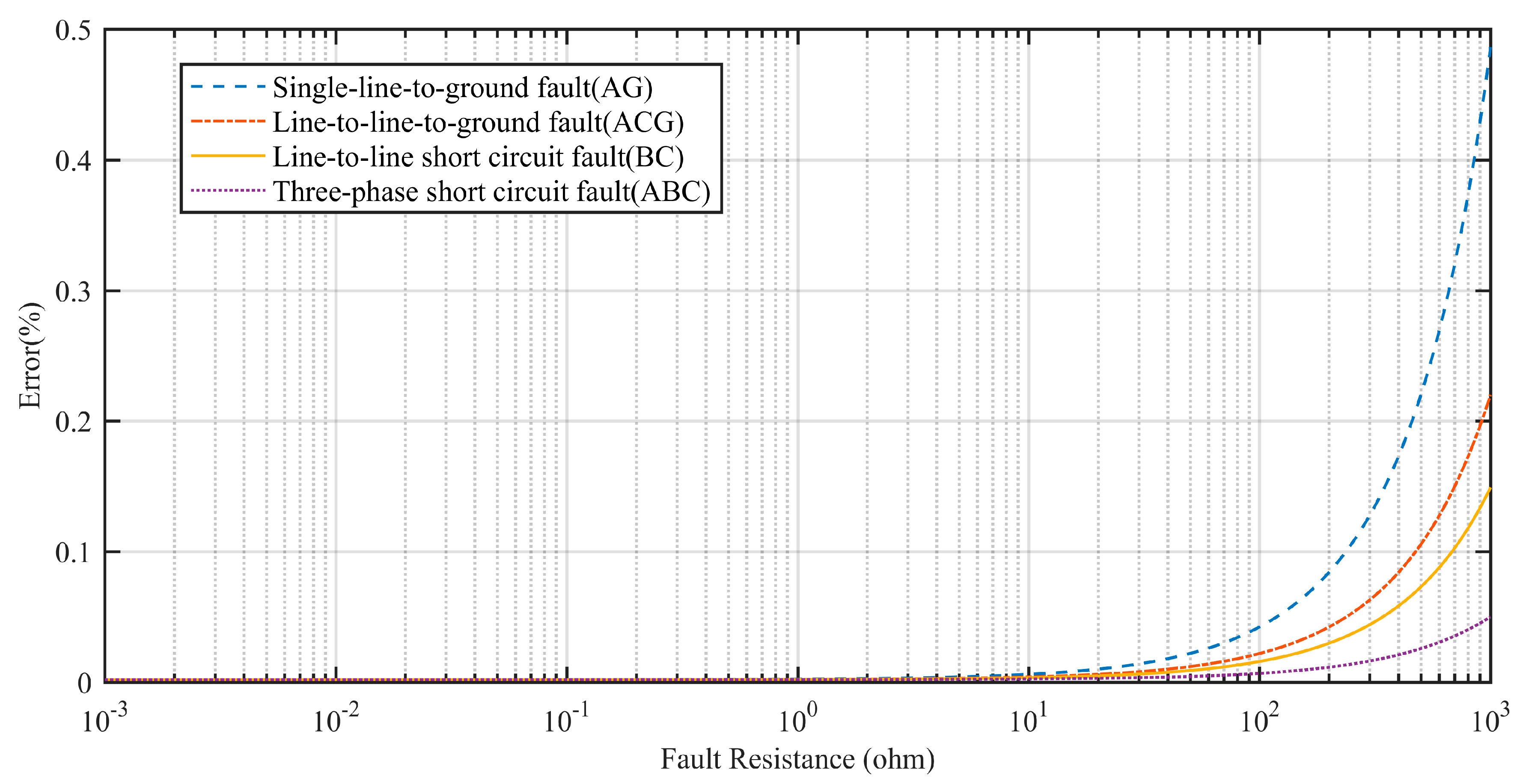
Tale 7 also shows the impact of a range of fault resistances on the location accuracy. When the fault inception angle is constant, as the fault resistance increases, the location accuracy decreases. Figure 13 shows the impact of the fault resistance. The errors for four fault types increase by different degrees with the growth of fault resistance. However, the fault location is accurate when the fault resistance is less than 100 Ω.

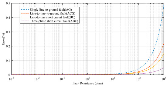
Figure 13. Impact of the fault resistance.

The location accuracy is mainly affected by the detection accuracy of the traveling wave arrival times. However, this is the inherent problem in the application of all traveling-wave-based fault location methods, which is restricted by the performance of TRs and their sampling frequency. This paper concentrates on the fault section identification technique and the corresponding location method in hybrid multi-terminal lines. To transiently detect the wavelet transform-based fault, more research is presented in other papers.

4.4. Comparison with Existing Methods

In order to show the advantages of the proposed method, we compared the presented method with several methods from previously published papers. The presented method is implemented using their benchmark datasets and the comparison with the existing methods are shown in Table 8, Table 9 and Table 10.

Table 8. Comparison with the existing methods in [29].

Method	Identified Faulty Section	Min Error (km)	Max Error (km)	Applied Line Structure
[29]	Line segment	0.081	0.177	Type(b)
Proposed method	Three-terminal network	0.079	0.201	Type(a) & Type(b)

Table 9. Comparison with the existing methods in [30].

Method	Identified Faulty Section	Min Error (km)	Max Error (km)	Applied Line Structure
[30]	-	0.010	0.040	Type(a)&Type(b)
Proposed method	Three-terminal network	0.005	0.022	Type(a)&Type(b)

Table 10. Comparison with the existing methods in [27].

Method	Identified Faulty Section	Min Error (km)	Max Error (km)	Applied Line Structure
[27]	Fault line	0.004	0.225	Type(a)
Proposed method	Three-terminal network	0.001	0.146	Type(a)&Type(b)

In Table 8, compared with the method in [29], although the range of the identified faulty section is bigger than the previous method, the proposed method offers a similar fault location accuracy. The error is less than 0.201 km which meets the application requirements. Further, the fault section identification procedure is simpler. In addition, both methods can be applied to multi-terminal radial structure types (b), but the proposed method also fits type (a). The multi-terminal radial structure type (a) and type (b) are shown in Figure 1.

In Table 9, compared with the method in [30], the proposed method locates faults more accurately. In the previous method, the fault point was located without identifying the faulty section. In addition, the location accuracy depended on the resolution of the position index in lines, which was the reason for the low accuracy.

In Table 10, compared with the method in [27], the proposed method obtains higher accuracy and it is suitable for both line structures. However, the method in [27] is infeasible because the branches have no common joint point for type (b). In summary, the proposed method is not influenced by the structure of the line model and has the higher accuracy for fault location.

5. Conclusions

Traveling-wave based fault location in complex line structures is an important issue and needs further improvement. In this paper, a new multi-terminal fault location method for hybrid multi-terminal lines has been proposed. By using the normalization algorithm, the impact of different line parameters has been eliminated in the proposed method. For the normalized multi-terminal lines, only the first three arrival times are directly applied in the proposed method to identify a three-terminal fault section, which is different from other methods. Consequently, the fault can be located in the fault section. The proposed fault location procedure is simple in terms of computational complexity compared with the previous methods and the fault location accuracy is improved. The effectiveness of the proposed method has been confirmed through test cases under different fault conditions. The simulation results have demonstrated that the proposed fault location method with simple computation is more accurate and can be applied to all multi-terminal structures.

References

- Ou, T.C.; Lu, K.H.; Huang, C.J. Improvement of transient stability in a hybrid power multi-system using a designed NIDC (novel intelligent damping controller). Energies 2017, 10, 488. [Google Scholar] [CrossRef]
- Souza, D.P.M.D.; Christo, E.S.; Almeida, A.R. Location of Faults in Power Transmission Lines Using the ARIMA Method. Energies 2017, 10, 1596. [Google Scholar] [CrossRef]
- Liang, R.; Yang, Z.; Peng, N.; Liu, C.L.; Zare, F. Asynchronous Fault Location in Transmission Lines Considering Accurate Variation of the Ground-Mode Traveling Wave Velocity. Energies 2017, 10, 1957. [Google Scholar] [CrossRef]
- Gana, N.; Aziz, N.A.; Ali, Z. A Comprehensive Review of Fault Location Methods for Distribution Power System. Indones. J. Electr. Eng. Comput. Sci. 2017, 6, 185–192. [Google Scholar] [CrossRef]
- Mahamedi, B.; Sanaye-Pasand, M.; Azizi, S.; Zhu, J.G. Unsynchronised fault-location technique for three-terminal lines. IET Gener. Transm. Distrib. 2015, 9, 2099–2107. [Google Scholar] [CrossRef]
- Namdari, F.; Salehi, M. Fault classification and location in transmission lines using traveling waves modal components and continuous wavelet transform CWT. J. Electr. Syst. 2016, 12, 373–386. [Google Scholar]
- Evrenosoglu, C.Y.; Abur, A. Travelling wave based fault location for teed circuits. IEEE Trans. Power Deliv. 2005, 20, 1115–1121. [Google Scholar] [CrossRef]
- Yadav, A.; Swetapadma, A. Enhancing the performance of transmission line directional relaying, fault classification and fault location schemes using fuzzy inference system. IET Gener. Transm. Distrib. 2015, 9, 580–591. [Google Scholar] [CrossRef]
- Das, S.; Santoso, S.; Gaikwad, A.; Patel, M. Impendence-based fault location in transmission network: Theory and application. IEEE Access 2014, 2, 537–557. [Google Scholar] [CrossRef]
- Liu, C.W.; Lin, T.C.; Yu, C.S.; Yang, J.Z. A fault location technique for two-terminal multisection compound transmission lines using synchronized phasor measurements. IEEE Trans. Smart Grid 2012, 3, 113–121. [Google Scholar] [CrossRef]
- Lien, K.P.; Liu, C.W.; Yu, C.S.; Jiang, J.A. Transmission network fault location observability with minimal PMU placement. IEEE Trans. Power Deliv. 2006, 21, 1128–1136. [Google Scholar] [CrossRef]
- Lin, W.M.; Ou, T.C. Unbalanced distribution network fault analysis with hybrid compensation. IET Gener. Transm. Distrib. 2010, 5, 92–100. [Google Scholar] [CrossRef]
- Ou, T.C. Ground fault current analysis with a direct building algorithm for microgrid distribution. Int. J. Electr. Power Energy Syst. 2013, 53, 867–875. [Google Scholar] [CrossRef]
- Ou, T.C. A novel unsymmetrical faults analysis for microgrid distribution systems. Int. J. Electr. Power Energy Syst. 2012, 43, 1017–1024. [Google Scholar] [CrossRef]
- Personal, E.; García, A.; Parejo, A. A Comparison of Impedance-Based Fault Location Methods for Power Underground Distribution Systems. Energies 2016, 9, 1022. [Google Scholar] [CrossRef]
- Argyropoulos, P.E.; Lev-Ari, H. Wavelet Customization for Improved Fault-Location Quality in Power Networks. IEEE Trans. Power Deliv. 2015, 30, 2215–2223. [Google Scholar] [CrossRef]
- Coffeen, L.; Mcbride, J.; Cantrelle, D. Initial Development of EHV Bus Transient Voltage Measurement: An Addition to On-line Transformer FRA. In Proceedings of the EPRI Substation Equipment Diagnostics Conference, Orlando, FL, USA, 2–5 March 2008. [Google Scholar]
- Chang, B.; Cwikowski, O.; Barnes, M.; Shuttleworth, R.; Beddard, A.; Coventry, P. Review of different fault detection methods and their impact on pre-emptive vsc-hvdc dc protection performance. High Volt. 2018, 2, 211–219. [Google Scholar] [CrossRef]
- Huang, S.J.; Liu, X.Z.; Su, W.F.; Ou, T.C. Application of enhanced honey-bee mating optimization algorithm to fault section estimation in power systems. IEEE Trans. Power Deliv. 2013, 28, 1944–1951. [Google Scholar] [CrossRef]
- Lin, S.; He, Z.Y.; Li, X.P. Travelling wave time-frequency characteristic-based fault location method for transmission lines. IET Gener. Transm. Distrib. 2012, 6, 764–772. [Google Scholar] [CrossRef]
- Lopes, F.V.; Fernandes, D.; Neves, W.L.A. A traveling-wave detection method based on Park’s transformation for fault locators. IEEE Trans. Power Deliv. 2013, 28, 1626–1634. [Google Scholar] [CrossRef]
- Lopes, F.V. Setting-free traveling-wave-based earth fault location using unsynchronized two-terminal data. IEEE Trans. Power Deliv. 2016, 31, 2296–2298. [Google Scholar] [CrossRef]
- Livani, H.; Evrenosoglu, C.Y. A fault classification and localization method for three-terminal circuits using machine learning. IEEE Trans. Power Deliv. 2013, 28, 2282–2290. [Google Scholar] [CrossRef]
- Lee, J.W.; Kim, W.K.; Han, J.; Jang, W.H.; Kim, C.H. Fault area estimation using traveling wave for wide area protection. J. Mod. Power Syst. Clean Energy 2016, 4, 478–486. [Google Scholar] [CrossRef]
- Zhang, S.; Zou, G.; Huang, Q.; Gao, H.L. A Traveling-Wave-Based Fault Location Scheme for MMC-Based Multi-Terminal DC Grids. Energies 2018, 11, 401. [Google Scholar] [CrossRef]
- Liang, R.; Cui, L.H.; Du, Z.L.; Li, G.X.; Fu, G.Q. Fault line selection and location in distribution power network based on traveling wave time difference of arrival relationships. High Volt. Eng. 2014, 40, 3411–3417. [Google Scholar]
- Hamidi, R.J.; Livani, H. Traveling-Wave-Based Fault-Location Algorithm for Hybrid Multiterminal Circuits. IEEE Trans. Power Deliv. 2017, 32, 135–144. [Google Scholar] [CrossRef]
- Sun, K.; Chen, Q.; Zhao, P. Automatic Faulted Feeder Section Location and Isolation Method for Power Distribution Systems Considering the Change of Topology. Energies 2017, 10, 1081. [Google Scholar] [CrossRef]
- Zhu, Y.; Fan, X. Fault location scheme for a multi-terminal transmission line based on current traveling waves. Int. J. Electr. Power Energy Syst. 2013, 53, 367–374. [Google Scholar] [CrossRef]
- Robson, S.; Haddad, A.; Griffiths, H. Fault location on branched networks using a multiended approach. IEEE Trans. Power Deliv. 2014, 29, 1955–1963. [Google Scholar] [CrossRef]
- Jensen, C.F. Fault in Transmission Cables and Current Fault Location Methods. In Location of Faults on AC Cables in Underground Transmission Systems; Springer: Basel, Switzerland, 2014; pp. 7–18. [Google Scholar]
- Livani, H.; Evrenosoglu, C.Y. A machine learning and wavelet-based fault location method for hybrid transmission lines. IEEE Trans. Smart Grid 2014, 5, 51–59. [Google Scholar] [CrossRef]
- Magnago, F.H.; Abur, A. Fault location using wavelets. IEEE Trans. Power Deliv. 1998, 13, 1475–1480. [Google Scholar] [CrossRef]
- Lopes, F.V.; Dantas, K.M.; Silva, K.M.; Costa, F.B. Accurate Two-terminal transmission line fault location using traveling waves. IEEE Trans. Power Deliv. 2017, 1, 1–8. [Google Scholar] [CrossRef]
- Vermeulen, H.J.; Dann, L.R.; van Rooijen, J. Equivalent circuit modelling of a capacitive voltage transformer for power system harmonic frequencies. IEEE Trans. Power Deliv. 1995, 10, 1743–1749. [Google Scholar] [CrossRef]
- Korkali, M.; Abur, A. Optimal Deployment of Wide-Area Synchronized Measurements for Fault-Location Observability. IEEE Trans. Power Syst. 2013, 28, 482–489. [Google Scholar] [CrossRef]
- Farshad, M.; Sadeh, J. Transmission line fault location using hybrid wavelet-Prony method and relief algorithm. Int. J. Electr. Power Energy Syst. 2014, 61, 127–136. [Google Scholar] [CrossRef]
- Costa, F.B.; Monti, A.; Lopes, F.V.; Silva, K.M.; Jamborsalamati, P.; Sadu, A. Two-terminal traveling wave-based transmission line protection. IEEE Trans. Power Deliv. 2017, 33, 1382–1393. [Google Scholar] [CrossRef]
- Tzelepis, D.; Fusiek, G.; Dysko, A.; Niewczas, P.; Booth, C.; Dong, X.Z. Novel Fault Location in MTDC Grids with Non-Homogeneous Transmission Lines Utilizing Distributed Current Sensing Technology. IEEE Trans. Smart Grid 2017, 1–12. [Google Scholar] [CrossRef]
© 2018 by the authors. Licensee MDPI, Basel, Switzerland. This article is an open access article distributed under the terms and conditions of the Creative Commons Attribution (CC BY) license (http://creativecommons.org/licenses/by/4.0/).