Enhanced Voltage Stability Assessment Index Based Planning Approach for Mesh Distribution Systems

Abstract

This paper offers an enhanced voltage stability assessment index (VSAI) and loss minimalize condition (LMC) centered integrated planning approach. The proposed method aims at the simultaneous attainment of voltage stability, loss minimizations and various other related objectives with the employment of multiple distributed generation (DG) units, in mesh distribution systems (MDS). The approach presents two enhanced VSAI expressions based on a multiple-loops configured equivalent MDS model. The main objective of each VSAI expression is to find the weakest buses as potential candidates for single and multiple DG placements with initial optimal DG sizes for aimed objectives attainment in MDS. Later, mathematical expressions for LMC have been presented, based on equivalent MDS model. The LMC aims to achieve significant loss minimization with optimal DG sizes and attain negligible voltage difference across tie-line branches via reduction of respective loop currents. The proposed integrated VSAI-LMC based planning approach is employed with two computation variants and tested on two well-known, 33-Bus and 69-Bus, test distribution systems (TDS). The performance analysis of each TDS is conducted with two cases and respective scenarios, across various performance evaluation indicators (PEIs). The paper also offers a comparative analysis of achieved numerical outcomes of the proposed planning approach with the available research works found in the literature. The numerical results attained have better performance in comparison with the presented literature data and thus shows the effectiveness and validity of the proposed planning approach.

1. Introduction

In distribution system (DS) planning and operation stages, steady voltage stability across feeders and power (both active and reactive) loss minimization are the foremost important issues that must be addressed as a priority. The increase of load requirements in large areas (mostly urban and suburbs) has also contributed to the degradation of power quality and stability along with the aforementioned technical issues. Among the major efforts to solve the aforesaid problems, distribution system planners and operators give key consideration to distributed generator (DG) units, in terms of optimal sitting and sizing in the DS [1]. The DG unit can impact a DS from the viewpoint of voltage profiles (U-profiles), power quality (at utilities and consumers end) and stability (transient and steady-state), short-circuit-current (SCC) levels, modified power flows and system reliability [2]. Traditionally, DS is always intentionally designed and planned to work under radial topology, mainly to retain unidirectional power flow. The radial distribution systems (RDS) being passive, are mostly favored around the globe due to relaxed (simple) control and protection requirements. Likewise, DG integration has neither considered in planning phase nor facilitated in the operational phase of RDS in traditional grid planning paradigm. The main factors considered in the DG planning problem include the DG-type, quantity, size, site, network topology and capacity of the existing DS [3].

The DS, on the basis of structural topology, is commonly categorized into radial, loop and mesh configurations. Irrespective of the linear employed protection arrangements, the RDS is inclined towards reliability, losses, voltage regulation and other associated issues. In comparison, single loop arranged distribution systems (LDS) and multiple-loop arranged mesh distribution systems (MDS) show improved reliability in addition to enhanced voltage profile stability along with the dedicated feeders [4]. Even though LDS and MDS are interconnected in nature, they require complicated protection schemes, are liable to small SCC levels, fault traceability and renewable energy generation (REG) integration issues. However, the aforesaid issues are expected to meet under smart grid (SG) philosophy, unlike the traditional grid paradigm. The concept of SG also involves the modernization of distribution system planning, associated functions, retained by most advanced SG technology and aims to improve the performance of future DS [5,6].

The significant difference between LDS and MDS is the number of exhibited loops. The RDS can be converted to LDS and MDS on the basis of closing normally-open (NO) tie-switches (TS). The LDS indicates a topology unlike RDS, any specific load on a bus is fed from two ends in a single loop (by closing one selected TS in DS). In the same way, in MDS, the load on a bus may be fed from two or more ends, by closing two or more TS in a multiple loop arrangement. This plan is more feasible in terms of cost since it employs existing infrastructure. These topologies are more suitable for urban centers and densely populated zones, which directly contributes to increased load level on the distribution side. Nonetheless, LDS and MDS are not as prominent as their radial counterparts and therefore can be used as a research motivation for investigating on the basis of performance assessments [4,5,6,7].

Besides topology, integration of DG near load centers has transformed DS from passive to an active distribution system (ADS). As aforementioned that RDS was not planned to integrate DGs. Thus the modernization of DS in planning and operation with several DGs types has become a noticeable research dimension, as advocated in [7,8]. There are numerous outstanding benefits accredited to the optimal placement of DGs in DS, such as maximizing load capacity, substation capacity relief, reliability, system efficiency, stability margins and the minimization of active/reactive losses, associated costs and thermal load of feeder. Hence, grid modernization based on DS topology (configuration) perspective is one of the main driving forces behind smart distribution system (SDS) planning and operation as mentioned in [8], to maximize the benefits associated with DG integration. In addition, SDS under SG is perceived as interconnected in organization and smart from planning and operational viewpoint. In ADS, the maximum achievable distribution of load is normally limited by the static voltage rather than the thermal boundary [9].

The literature review points out a large amount of research that is applied to achieving various goals with DG based planning aiming at RDS. In most of the studies, the radial topology of DS is retained as a problem constraint. Various researchers have reviewed DG allocations in DS on the basis of site, size, type, application and planning. The most significant classes of optimal DG placement (sitting and sizing) include methods such as numerical, analytic, artificial intelligence, meta-heuristics, hybrid algorithms and various miscellaneous techniques [1,2,3,6,7,8,10,11,12]. Likewise, analytical and numerical-based methods detailed in References [13,14,15,16,17,18,19,20,21,22]. Optimal DG sitting and sizing have been considered important planning tools, which are designed to achieve a trade-off solution among multiple conflicting objectives. A bibliographic investigation aims to minimize losses in RDS, with DG sitting, capacitor placement and network reconfiguration proposed in Reference [23]. DG placement as a potential planning substitute for RDS has been encouraged regarding loss minimizations and voltage stability, as reviewed in [24,25]. Numerous DG (sitting and sizing), reinforcements and planning components based planning problems are reviewed in References [26,27].

In addition to DG allocation based planning, the review of recent literature also shows that there is a considerable amount of research work available from the perspective of loop/mesh topology in DS. A viability study has been discussed in Reference [28], which primarily focuses on upgrading the radial topology into different types of loops and is supported by numerous performance evaluations. Likewise, a multi-stage planning methodology based on a sensitivity based approach and a non-dominated sorting genetic algorithm II (NSGA-II), aiming at optimal DG sitting and sizing in LDS is offered in Reference [29]. The influence of loops by number and their impact in MDS under different load models (along with load growth) is demonstrated in Reference [30]. A notable research work based on the sensitivity method and aiming at optimal DG sitting and sizing within MDS, under time-varying load models is demonstrated in Reference [31]. A comparative study using four approaches is presented in Reference [32], in which the main objective is to increase DG penetration by replacing the TS with fault current limiter (FCL), within MDS respectively. An integrated planning approach along with an improved variant is presented in References [33,34], comprising of graph-partitioning and integer-programming, aims to address operational efficiency and reliability perspectives with a micro-grid (MG) topology planning (MTP) method to optimize the LDS based MG structure.

A multiple-objective optimization based framework is offered to upgrade the LDS into MDS as shown in Reference [35]. In Reference [36], a comprehensive economic analysis is proposed to upgrade RDS to LDS, by employing optimal site and number of FCL, along with finding a feasible solution between the reliability and minimization of system losses. A voltage stability index (VSI) centered-methodology is proposed in Reference [37] to evaluate the voltage stability of single loop based LDS. Furthermore, the VSI centered-method and loss minimalize condition (LMC) based integrated planning approach is recommended for single loop configured LDS in Reference [38]. The approach in Reference [38] aims at simultaneously achieving an increase in optimal DG penetration, voltage maximization (U_Max), loss minimization (L_Min) in a single loop based LDS, and is supported by evaluations of various performance metrics. A circuit-based-theory L-min approach is proposed for ADS configured in interconnected topology [39].

It is pointed out in Reference [40] that the voltage magnitude alone is not a suitable measure for the voltage stability assessment (VSA) of a DS. Several VSA-based indices are accessible in the literature, which aim at optimizing the DG (site and size) layout in RDS. These indices (mostly voltage centered) are based on equivalent two-bus and single branch model for the representation of an equivalent RDS model. In addition, voltage assessment based indices for RDS are not suitable for the LDS and MDS, from the perspective of the application. Similarly, VSI for single loop based LDS (two-branch model) can show some limitations for multi-loop configured MDS. Reason-being, the VSI method, established as equivalent to the two branch model in Reference [37], cannot prove and fulfill all aspects of MDS. For example, a bus in multiple loop MDS can be fed by two or more sending-end (SB) buses (in multi-branch MDS model) and the assumption that load is fed from two SB at maximum (in two branch model in LDS), does not remain justified in MDS. Moreover, in the aforementioned publications, a voltage stability index (VSI) based dedicated method for simultaneously achieving U_Max, L_Min and optimal DG penetration, the evaluation of performance under different metrics and covering all the aspects of an equivalent multiple-loop based MDS model, have not been addressed. Hence, addressing the research gap in the presented literature is the driving force for our research and serves as the motivation of the work in this paper.

In this research paper, two enhanced and dedicated VSIs are proposed, which cover most aspects of the equivalent MDS model. The limitations in VSI (for LDS) presented in our previous publications [37,38] and reviewed literature (from the perspective of VSI for MDS and DG placement), is the key inspiration for the derivation of proposed indices that are capable of evaluating multi-loop configured MDS. In order to avoid confusion among various VSA (or VSI) indices from previous works, this paper employs the term voltage stability assessment index (VSAI) for MDS instead of VSI. Moreover, an improved loss minimalizing condition (LMC) for an equivalent MDS is also proposed. The LMC in our previous work [38] is limited to a single loop LDS model. The paper also offers an improved VSAI and LMC based integrated planning approach for optimal multiple-DG (sitting and sizing) placements in MDS. The VSAI-LMC approach is evaluated under various performance metrics. The key contributions of the proposed research are as follows:

(i)

Two derived mathematical expressions of VSAIs for equivalent electrical MDS models.

(ii)

Mathematical expression for improved LMC for an equivalent MDS model.

(iii)

Integrated planning approach (VSAI-LMC) for MDS is applied with two computation variants.

(iv)

Evaluation of proposed planning approach on two (33-Bus and 69-Bus) test DS.

(v)

Evaluation of proposed planning approach under multiple DG placements (sitting and sizing).

(vi)

Evaluation of proposed planning approach under various performance metrics.

(vii)

Validation of proposed approach by comparison of results with works available in the literature.

This article is arranged as follows: Section 2 presents the comprehensive mathematical derivations of two VSAIs expressions for MDS; Section 3 offers LMC expressions for both active and reactive components within MDS; the computation procedure for the VSAI-LMC based planning approach, simulation setup and evaluation indicators are illustrated in Section 4; in Section 5, the attained numerical results regarding the effectiveness of the proposed approach is evaluated with multiple DG (sitting and size) viewpoints and assessment (with discussion), performed under various performance metrics, is demonstrated on two test distribution systems; the comparison of the proposed planning approach with existing research work for validation is presented in Section 6; the conclusion of the paper is offered in Section 7.

2. Voltage Stability Assessment Indices for Mesh Distribution System

2.1. Background: Reference Based Voltage Stability Index for Loop Distribution System

In this work, the VSI for single loop configured LDS that is derived from our earlier publications [37,38] is used as a reference standard. The relevant VSI in Reference [37] is based on biquadratic method and VSI-LMC planning method is used for single loop LDS optimization. Besides comparison, the VSI in References [37,38] has been engaged to find out effectiveness of proposed VSAIs via comparison of attained results. In literature, it is designated with term VSI_L. The electrical equivalent LDS model is shown in Figure 1, which is based on three-wire equivalent distribution system, also considered in References [4,37,38].

A type-I loop topology, as advocated in Reference [28], is considered due to its simplicity and feasibility, where two radial feeders (branches) are joined to make a closed-loop and are fed by the same power transformer. Details on the VSI_L can be found in Reference [37]. The expressions for VSI_L and relevant feasible voltage solution on receiving end bus (U_RBI), are shown in Equations (1) and (2).

$$\begin{gathered} \mathrm{V}\mathrm{S}\mathrm{I}\_\mathrm{L}=\mathrm{V}\mathrm{S}\mathrm{I}{(m_{2b})}_{\mathrm{L}\mathrm{D}\mathrm{S}}={{\displaystyle \sum }}_{i=1}^{nb{s}_l}{\left[\frac{\left|U_{nbs}\right|}{nb{s}_l}\right]}^4-2{{\displaystyle \sum }}_{i=1}^{nb{s}_l}{\left[\frac{\left|U_{nbs}\right|}{nb{s}_l}\right]}^2\left[\left[\frac{E}{(R_{1r}+∆R_r)}\right]+\left[\frac{F}{(X_{1x}+∆X_x)}\right]\right]- \\ {\left[\frac{E}{(R_{1r}+∆R_r)}-\frac{F}{(X_{1x}+∆X_x)}\right]}^2\ge 0 \end{gathered}$$

(1)

where U_nbs are the sending end (SB) bus voltages, nbs_l is the number of SB, receiving end bus (RB) bus, tie-line-branch (TB), tie-switch (TS) and I_TB is the TB current, as shown in LDS in Figure 1. E = P_2b (R_1rR_3r − X_1xX_3x) + Q_2b (R_1rX_3x + R_3rX_1x) and F = P_2b (R_1rX_3x + R_3rX_1x) − Q_2b (R_1rR_3r − X_1xX_3x). [Z_1z + ΔZ] is a mutual term, |ΔZ| = |Z_1z − Z_3z| ≥ 0 is assumed for open branches in LDS, |ΔZ| = Z_3z for TB, feeding node m_4b from another node (m_2b), as shown in Equations (1) and (2).

$$\left|U_{RBI}\right|=0.707\sqrt{\begin{array}{c}\left\{{\displaystyle {\displaystyle \sum }_{i=1}^{nb{s}_l}}{\left[\frac{\left|U_{nbs}\right|}{nb{s}_l}\right]}^2-\left[\frac{E}{(R_{1r}+∆R_r)}\right]+\left[\frac{F}{(X_{1x}+∆X_x)}\right]\right\}\\ +\sqrt{{\displaystyle {\displaystyle \sum }_{i=1}^{nb{s}_l}}{\left[\frac{\left|U_{nbs}\right|}{nb{s}_l}\right]}^4-2{\displaystyle {\displaystyle \sum }_{i=1}^{nb{s}_l}}{\left[\frac{\left|U_{nbs}\right|}{nb{s}_l}\right]}^2\left[\left[\frac{E}{(R_{1r}+∆R_r)}\right]+\left[\frac{F}{(X_{1x}+∆X_x)}\right]\right]-{\left[\frac{E}{(R_{1r}+∆R_r)}-\frac{F}{(X_{1x}+∆X_x)}\right]}^2\ge 0}\end{array}}$$

(2)

2.2. Proposed Voltage Stability Assessment Index for Mesh Distribution System under Ideal Case (VSAI_MI)

VSAI from the perspective of an ideal MDS electrical equivalent model is denoted with the term VSAI_MI and corresponds to an arrangement, which assumes that the TB along with respective TS may have small impedance and can be represented by a single load. Also, the three buses feeding the respective load are assumed at same voltage potential and are represented as one source originating from the substation (SS). These assumptions decrease the MDS model to a simplified system, as shown in Figure 2. The ideal MDS model consists of five branches. Three branches correspond to distribution feeders and two tie-line branches connect them together. When the respective TS, as shown in Figure 3 as TS1 and TS2 and closed, the RDS system can be converted into multiple-loop encapsulated MDS. It is assumed that voltages (U) across sending end buses (SBs such as m_1b, m_3b and m_5b) are the same, with zero difference of U and phase (δ), and are shown as connected loops at sending end buses to show one source bus m_1b.

On receiving end buses (RBs such as m_2b, m_4b and m_6b), TB (TB1 between m_2b and m_4b, TB2 between m_2b and m_6b) and TS (TS1 between m_2b and m_4b, TS2 between m_2b and m_6b) are assumed to have negligible impedance and are thus ignored. The loads on the RBs (S_2b, S_4b and S_6b) at respective nodes are assumed to be added up single lumped load at RE m_2b, which is S_B as shown in Figure 3. The voltages at RBs (U_2b, U_4b and U_6b) are also considered at the same level and are represented with U_2b. The system shown in Figure 3 considers most of the aspects of an ideal MDS. The total apparent (load) power S_B at node m_2b can be written in the form of Equation (3), as follows:

$$S_B=S_{2b}+S_{4b}+S_{6b}={\left[P_{2B}+j{Q}_{2B}\right]}^{*}=U_{2b}{\left(I_{1B}+I_{2B}+I_{3B}\right)}^{*}$$

(3)

Currents $I_{1B}, I_{2B}, \mathrm{and} I_{3B}$ refer to the branches 1, 2 and 3, in ideal MDS. The total net apparent power in terms of the voltage difference across respective RBs and respective impedances can be rewritten in Equation (4).

$${S_B}^{*}=\left[P_{2B}-j{Q}_{2B}\right]={U_{2b}}^{*}\left[\frac{U_{1b}-U_{2b}}{{\mathrm{\mathbb{Z}}}_{1B}}+\frac{U_{1b}-U_{2b}}{{\mathrm{\mathbb{Z}}}_{2B}}+\frac{U_{1b}-U_{2b}}{{\mathrm{\mathbb{Z}}}_{3B}}\right]$$

(4)

On the basis of assumptions, the voltages across two TB are considered to be the same, that is, $U_{2b}=U_{4b}=$ $U_{6b}$. The impedances of respective distribution branches are illustrated as, ${\mathrm{\mathbb{Z}}}_{1B}=R_{1r}+j{X}_{1x}, {\mathrm{\mathbb{Z}}}_{2B}=R_{2r}+j{X}_{2r}$ and ${\mathrm{\mathbb{Z}}}_{3B}=R_{3r}+j{X}_{3r}$. The Equation (4) can be rearranged as Equation (5):

$$\left[P_{2B}-j{Q}_{2B}\right]=\left[\left|U_{1b}\right|\left|U_{2b}\right|\angle {\mathsf{\delta }}_{1b}-{\mathsf{\delta }}_{2b}-{\left|U_{2b}\right|}^2\right]\left[\frac{1}{{\mathrm{\mathbb{Z}}}_{1B}}+\frac{1}{{\mathrm{\mathbb{Z}}}_{2B}}+\frac{1}{{\mathrm{\mathbb{Z}}}_{3B}}\right]$$

(5)

The Equation (5) is reorganized as follows:

$$\left[P_{2B}-j{Q}_{2B}\right]=\left[\left|U_{1b}\right|\left|U_{2b}\right|\angle {\mathsf{\delta }}_{1b}-{\mathsf{\delta }}_{2b}-{\left|U_{2b}\right|}^2\right]\left[\frac{{\mathrm{\mathbb{Z}}}_{1B}{\mathrm{\mathbb{Z}}}_{2B}+{\mathrm{\mathbb{Z}}}_{1B}{\mathrm{\mathbb{Z}}}_{3B}+{\mathrm{\mathbb{Z}}}_{2B}{\mathrm{\mathbb{Z}}}_{3B}}{{\mathrm{\mathbb{Z}}}_{1B}{\mathrm{\mathbb{Z}}}_{2B}{\mathrm{\mathbb{Z}}}_{3B}}\right]$$

(6)

The Equation (6) is reordered in the form of left-hand-side (L-H-S) and right-hand-side (R-H-S) in Equation (7) becomes:

$$\left[P_{2B}-j{Q}_{2B}\right]\left[{\mathrm{\mathbb{Z}}}_{1B}{\mathrm{\mathbb{Z}}}_{2B}{\mathrm{\mathbb{Z}}}_{3B}\right]=\left[\left|U_{1b}\right|\left|U_{2b}\right|\angle {\mathsf{\delta }}_{1b}-{\mathsf{\delta }}_{2b}-{\left|U_{2b}\right|}^2\right]\left[{\mathrm{\mathbb{Z}}}_{1B}{\mathrm{\mathbb{Z}}}_{2B}+{\mathrm{\mathbb{Z}}}_{1B}{\mathrm{\mathbb{Z}}}_{3B}+{\mathrm{\mathbb{Z}}}_{2B}{\mathrm{\mathbb{Z}}}_{3B}\right]$$

(7)

The Equation (7) is again extended in-terms of resistance and reactance is arranged in Equation (8).

$$\left[P_{2B}-j{Q}_{2B}\right]\left[\left(R_{1r}+j{X}_{1x}\right)\left(R_{2r}+j{X}_{2x}\right)\left(R_{3r}+j{X}_{3x}\right)\right]=[\left|U_{1b}\right|\left|U_{2b}\right|\angle {\mathsf{\delta }}_{1b}-{\mathsf{\delta }}_{2b}-{\left|U_{2b}\right|}^2]\left[\left(R_{1r}+j{X}_{1x}\right)\left(R_{2r}+j{X}_{2x}\right)+\left(R_{1r}+j{X}_{1x}\right)\left(R_{3r}+j{X}_{3x}\right)+\left(R_{2r}+j{X}_{2x}\right)\left(R_{3r}+j{X}_{3x}\right)\right]$$

(8)

The L-H-S in Equation (8) is segregated in-terms of real and imaginary parts. The real part of L-H-S product is labeled as E = Re $\left|\left[P_{2B}-j{Q}_{2B}\right]\left[\left(R_{1r}+j{X}_{1x}\right)\left(R_{2r}+j{X}_{2x}\right)\left(R_{3r}+j{X}_{3x}\right)\right]\right|$ as rearranged in generalized expression as shown in Equation (9a).

$$\begin{gathered} E=P_{2B}\left[{\displaystyle \prod }_{i=1}^m{R}_{mr}\right]\left[1-\left(\frac{X_{1x}{X}_{2x}}{R_{1r}{R}_{2r}}+\frac{X_{1x}{X}_{3x}}{R_{1r}{R}_{3r}}+\frac{X_{2x}{X}_{3x}}{R_{2r}{R}_{3r}}\right)\right] \\ +Q_{2B}\left[{\displaystyle \prod }_{i=1}^m{X}_{mx}\right]\left[\left(\frac{R_{1r}{R}_{2r}}{X_{1x}{X}_{2x}}+\frac{R_{1r}{R}_{3r}}{X_{1x}{X}_{3x}}+\frac{R_{2r}{R}_{3r}}{X_{2x}{X}_{3x}}\right)-1\right] \end{gathered}$$

(9a)

Imaginary part of Equation (8) is labeled as F = Im $\left|\left[P_{2B}-j{Q}_{2B}\right]\left[\left(R_{1r}+j{X}_{1x}\right)\left(R_{2r}+j{X}_{2x}\right)\left(R_{3r}+j{X}_{3x}\right)\right]\right|$, as in generalized expression as Equation (9b).

$$\begin{gathered} F=P_{2B}\left[{\displaystyle \prod }_{i=1}^m{X}_{mx}\right]\left[\left(\frac{R_{1r}{R}_{2r}}{X_{1x}{X}_{2x}}+\frac{R_{1r}{R}_{3r}}{X_{1x}{X}_{3x}}+\frac{R_{2r}{R}_{3r}}{X_{2x}{X}_{3x}}\right)-1\right] \\ -Q_{2B}\left[{\displaystyle \prod }_{i=1}^m{R}_{mr}\right]\left[1-\left(\frac{X_{1x}{X}_{2x}}{R_{1r}{R}_{2r}}+\frac{X_{1x}{X}_{3x}}{R_{1r}{R}_{3r}}+\frac{X_{2x}{X}_{3x}}{R_{2r}{R}_{3r}}\right)\right] \end{gathered}$$

(9b)

The R-H-S in Equation (8) is segregated in the same way as shown in Equations (9a) and (9b). The modified expression for the real part of R-H-S of Equation (8) is shown in Equation (10a) as follows:

$$E=[\left|U_{1b}\right|\left|U_{2b}\right|\cos \angle {\mathsf{\delta }}_{1b}-{\mathsf{\delta }}_{2b}-{\left|U_{2b}\right|}^2]\left[abs\left\{\left(R_{1r}{R}_{2r}+R_{1r}{R}_{3r}+R_{2r}{R}_{3r}\right)-\left(X_{1x}{X}_{2x}+X_{1x}{X}_{3x}+X_{2x}{X}_{3x}\right)\right\}+\Delta A\right]$$

(10a)

The $\Delta A$ is the amendment factor to avoid any unrequired condition such as not-a-numerical-number (N-A-N) and its value is assumed to be set at 0.001. The generalized expression is shown in Equation (10b).

$$E=\left[\left|U_{1b}\right|\left|U_{2b}\right|\cos \angle {\mathsf{\delta }}_{1b}-{\mathsf{\delta }}_{2b}-{\left|U_{2b}\right|}^2\right]\left[abs\left\{{\displaystyle \sum }_{k\ne l}^m{R}_k{R}_l-{\displaystyle \sum }_{k\ne l}^m{X}_k{X}_l\right\}+\Delta A\right]$$

(10b)

For the sake of simplicity, the relationship-term $\left[abs\left\{{\displaystyle \sum }_{k\ne l}^m{R}_k{R}_l-{\displaystyle \sum }_{k\ne l}^m{X}_k{X}_l\right\}+\Delta A\right]$ is labeled as G. The modified crisp expression after rearrangement is shown in Equation (10c).

$$\frac{E}{G}=\left[\left|U_{1b}\right|\left|U_{2b}\right|\cos \angle {\mathsf{\delta }}_{1b}-{\mathsf{\delta }}_{2b}-{\left|U_{2b}\right|}^2\right]$$

(10c)

Similarly expression for the imaginary part of R-H-S of Equation (8) is shown in Equation (11a) as follows:

$$F=\left[\left|U_{1b}\right|\left|U_{2b}\right|\sin \angle {\mathsf{\delta }}_{1b}-{\mathsf{\delta }}_{2b}-{\left|U_{2b}\right|}^2\right]\left[abs\left(R_1{X}_2+R_2{X}_1+R_1{X}_3+R_3{X}_1+R_2{X}_3+R_3{X}_2\right)\right]$$

(11a)

For the simplification of expression, the term $abs\left(R_1{X}_2+R_2{X}_1+R_1{X}_3+R_3{X}_1+R_2{X}_3+R_3{X}_2\right)$ is labeled as H. The expression can also be written in the generalized term as H = $abs\left[{\displaystyle \sum }_{k\ne l}^m{R}_k{X}_l\right].$ The modified arrangement is shown in Equation (11b) as follows:

$$\frac{F}{H}=\left[\left|U_{1b}\right|\left|U_{2b}\right|\sin \angle {\mathsf{\delta }}_{1b}-{\mathsf{\delta }}_{2b}-{\left|U_{2b}\right|}^2\right]$$

(11b)

According to trigonometric property, the real and imaginary parts of Equation (8), as elaborated in Equations (10c) and (11b) are rearranged. By square and adding, the expression becomes:

$${\left[\left(\frac{E}{G}\right)+{\left|U_{1b}\right|}^2\right]}^2+{\left[\left(\frac{F}{H}\right)+{\left|U_{1b}\right|}^2\right]}^2={\left[\left|U_{1b}\right|\left|U_{2b}\right|\right]}^2$$

(12)

Reorganization of Equation (12) in accordance with of the biquadratic method, results in real root solution of the quadratic root (b² − 4ac > 0). The improved Equation for a feasible solution is shown in Equation (13). Where b = $0.5{\left|U_{1b}\right|}^2-\left\{\left(\frac{E}{G}\right)+\left(\frac{F}{H}\right)\right\}$ and c = $\frac{1}{2}\left[\left(\frac{E}{G}\right)+\left(\frac{F}{H}\right)\right]$.

$${\left|U_{2b}\right|}^4-\left[0.5{\left|U_{1b}\right|}^2-\left\{\left(\frac{E}{G}\right)+\left(\frac{F}{H}\right)\right\}\right]{\left|U_{2b}\right|}^2+\frac{1}{2}\left[\left(\frac{E}{G}\right)+\left(\frac{F}{H}\right)\right]=0$$

(13)

The achievable real root solution in Equation (13) after scaling by multiplication on both sides by 4, VSAI for an ideal MDS is rearranged as modified expression as shown in Equation (14). The rescaling of the Equation is intended to define a threshold value of VSAI value between 0 (instability) and 1 (stable).

$$\mathrm{V}\mathrm{S}\mathrm{A}\mathrm{I}\_\mathrm{M}\mathrm{I}={\left|U_{1b}\right|}^4-4{\left|U_{1b}\right|}^2\left[\left(\frac{E}{G}\right)+\left(\frac{F}{H}\right)\right]-4{\left[\left(\frac{E}{G}\right)-\left(\frac{F}{H}\right)\right]}^2\ge 0$$

(14)

The respective expressions of variables (E, F, G and H) are included in Equation (15) to illustrate the complete expression of VSAI for an ideal MDS, as designated by VSAI_MI.

$$\begin{array}{l}\mathrm{V}\mathrm{S}\mathrm{A}\mathrm{I}\_\mathrm{M}\mathrm{I}={\left|U_{1b}\right|}^4\\ -4{\left|U_{1b}\right|}^2\left[\right\{\frac{P_{2B}\left[{{\displaystyle \prod }}_{i=1}^m{R}_{mr}\right][1-\left(\frac{X_{1x}{X}_{2x}}{R_{1r}{R}_{2r}}+\frac{X_{1x}{X}_{3x}}{R_{1r}{R}_{3r}}+\frac{X_{2x}{X}_{3x}}{R_{2r}{R}_{3r}}\right)]+Q_{2B} \left[{{\displaystyle \prod }}_{i=1}^m{X}_{mx}\right]\left[\left(\frac{R_{1r}{R}_{2r}}{X_{1x}{X}_{2x}}+\frac{R_{1r}{R}_{3r}}{X_{1x}{X}_{3x}}+\frac{R_{2r}{R}_{3r}}{X_{2x}{X}_{3x}}\right)-1\right]}{\left[abs\left\{{{\displaystyle \sum }}_{k\ne l}^m{R}_k{R}_l-{{\displaystyle \sum }}_{k\ne l}^m{X}_k{X}_l\right\}+\Delta A\right]}\}\\ +\left\{\frac{P_{2B}\left[{{\displaystyle \prod }}_{i=1}^m{X}_{mx}\right] \left[\left(\frac{R_{1r}{R}_{2r}}{X_{1x}{X}_{2x}}+\frac{R_{1r}{R}_{3r}}{X_{1x}{X}_{3x}}+\frac{R_{2r}{R}_{3r}}{X_{2x}{X}_{3x}}\right)-1\right]-Q_{2B} \left[{{\displaystyle \prod }}_{i=1}^m{R}_{mr}\right]\left[1-\left(\frac{X_{1x}{X}_{2x}}{R_{1r}{R}_{2r}}+\frac{X_{1x}{X}_{3x}}{R_{1r}{R}_{3r}}+\frac{X_{2x}{X}_{3x}}{R_{2r}{R}_{3r}}\right)\right]}{abs\left[{{\displaystyle \sum }}_{k\ne l}^m{R}_k{X}_l\right]}\right\}]\\ -4\left[\right\{\frac{P_{2B}\left[{{\displaystyle \prod }}_{i=1}^m{R}_{mr}\right][1-\left(\frac{X_{1x}{X}_{2x}}{R_{1r}{R}_{2r}}+\frac{X_{1x}{X}_{3x}}{R_{1r}{R}_{3r}}+\frac{X_{2x}{X}_{3x}}{R_{2r}{R}_{3r}}\right)]+Q_{2B} \left[{{\displaystyle \prod }}_{i=1}^m{X}_{mx}\right]\left[\left(\frac{R_{1r}{R}_{2r}}{X_{1x}{X}_{2x}}+\frac{R_{1r}{R}_{3r}}{X_{1x}{X}_{3x}}+\frac{R_{2r}{R}_{3r}}{X_{2x}{X}_{3x}}\right)-1\right]}{\left[abs\left\{{{\displaystyle \sum }}_{k\ne l}^m{R}_k{R}_l-{{\displaystyle \sum }}_{k\ne l}^m{X}_k{X}_l\right\}+\Delta A\right]}\}\\ -\left\{\frac{P_{2B}\left[{{\displaystyle \prod }}_{i=1}^m{X}_{mx}\right] \left[\left(\frac{R_{1r}{R}_{2r}}{X_{1x}{X}_{2x}}+\frac{R_{1r}{R}_{3r}}{X_{1x}{X}_{3x}}+\frac{R_{2r}{R}_{3r}}{X_{2x}{X}_{3x}}\right)-1\right]-Q_{2B} \left[{{\displaystyle \prod }}_{i=1}^m{R}_{mr}\right]\left[1-\left(\frac{X_{1x}{X}_{2x}}{R_{1r}{R}_{2r}}+\frac{X_{1x}{X}_{3x}}{R_{1r}{R}_{3r}}+\frac{X_{2x}{X}_{3x}}{R_{2r}{R}_{3r}}\right)\right]}{\left[{{\displaystyle \sum }}_{k\ne l}^m{R}_k{X}_l\right]}\right\}{]}^2\ge 0\end{array}$$

(15)

The RB voltage (U_2b) at node m_2b (also shown with U_RBI) in ideal MDS case, pointing at a feasible solution is shown as $\left|U_{2b}\right|$ = $\sqrt{b+\sqrt{b^2-4ac}}$. The expressions for root containing scaled values of b = $\left[{\left|U_{1b}\right|}^2-2\left\{\left(\frac{E}{G}\right)+\left(\frac{F}{H}\right)\right\}\right]$ and VSAI relation for an ideal MDS is shown in Equation (16).

$$\left|U_{RBI}\right|=\left|U_{2b}\right|=\frac{1}{\sqrt{2}}\sqrt{\left[{\left|U_{1b}\right|}^2-2\left\{\left(\frac{E}{G}\right)+\left(\frac{F}{H}\right)\right\}\right]+{\left|U_{1b}\right|}^4-4{\left|U_{1b}\right|}^2\left[\left(\frac{E}{G}\right)+\left(\frac{F}{H}\right)\right]-4{\left[\left(\frac{E}{G}\right)-\left(\frac{F}{H}\right)\right]}^2}$$

(16)

2.3. Proposed Voltage Stability Assessment Index for Mesh Distribution System under Actual Case (VSAI_MA)

The VSAI for an actual MDS is denoted with term VSAI_MA and corresponds to a practical situation, assuming that the TBs and associated TSs may have significant impedance. Such MDS can be served by two or more sources from a single (same) substation. This means that the TB has a high R/X ratio such that the voltages at RBs (U_2b ≠ U_4b ≠ U_6b) cannot be considered at the same level and are not representable with single voltage source, unlike ideal case. Similarly, the SBs may have different voltage level moreover assumption of an ideal MDS is not applicable (U_1b ≠ U_3b ≠ U_5b).

The main aim of this derivation is to address the limitations left in an ideal MDS model. In order to simplify complex expressions, approximations have considered in the derivation. Figure 3 shows the electrical equivalent model of an actual MDS. However, the loading at bus m_2b is considered at a normal load S_2b, fed by two TS ends (m_4b and m_6b) via tie-branch currents (I_TB1 and I_TB2), besides dedicated serving source (m_1b). Therefore, the composite load power at the load node m_2b is written in Equation (17) as follows:

$$S_{2b}=U_{2b}{\left(I_1+I_{TB1}+I_{TB2}\right)}^{*}$$

(17)

I_1B is the current of distribution feeder (between nodes m_1b and m_2b) in actual MDS model, I_TB1 and I_TB2 and the tie-branch currents serving node m_2b. Where ${\mathrm{\mathbb{Z}}}_{1B}$, ${\mathrm{\mathbb{Z}}}_{TB1}$ and ${\mathrm{\mathbb{Z}}}_{TB2}$ are the respective impedances of the dedicated feeders and respective TB. The modified expression in-terms of voltage difference and impedances are shown in Equation (18). This consideration covers the actual MDS model.

$$\left[\left(P_{2b}-j{Q}_{b2}\right)\right]={U_{2b}}^{*}\left[\frac{U_{1b}-U_{2b}}{{\mathrm{\mathbb{Z}}}_{1B}}+\frac{U_{4b}-U_{2b}}{{\mathrm{\mathbb{Z}}}_{TB1}}+\frac{U_{6b}-U_{2b}}{{\mathrm{\mathbb{Z}}}_{TB2}}\right]$$

(18)

The extension, elaboration and simplification of Equation (18) by cross-multiplication, a result in modified relationship is shown in Equation (19a), as follows. Where ${\mathrm{\mathbb{Z}}}_{1B}=R_{1r}+j{X}_{1x}, {\mathrm{\mathbb{Z}}}_{TB1}=R_{TB1}+j{X}_{TB1}$ and ${\mathrm{\mathbb{Z}}}_{TB2}=R_{TB2}+j{X}_{TB2}$.

$$\begin{gathered} \left[\left(P_{2b}-j{Q}_{b2}\right)\right]\left[{\mathrm{\mathbb{Z}}}_{1B}{\mathrm{\mathbb{Z}}}_{TB1}{\mathrm{\mathbb{Z}}}_{TB2}\right] \\ =\left[\left|U_{1b}\right|\left|U_{2b}\right|\angle {\mathsf{\delta }}_{1b}-{\mathsf{\delta }}_{2b}-{\left|U_{2b}\right|}^2\right]\left[{\mathrm{\mathbb{Z}}}_{TB1}{\mathrm{\mathbb{Z}}}_{TB2}\right]+\left[\left|U_{4b}\right|\left|U_{2b}\right|\angle {\mathsf{\delta }}_{4b}-{\mathsf{\delta }}_{2b}-{\left|U_{2b}\right|}^2\right]\left[{\mathrm{\mathbb{Z}}}_{1B}{\mathrm{\mathbb{Z}}}_{TB2}\right] \\ +\left[\left|U_{6b}\right|\left|U_{2b}\right|\angle {\mathsf{\delta }}_{6b}-{\mathsf{\delta }}_{22b}-{\left|U_{2b}\right|}^2\right]\left[{\mathrm{\mathbb{Z}}}_{1B}{\mathrm{\mathbb{Z}}}_{TB1}\right] \end{gathered}$$

(19a)

The Equation (19a) is further extended and rearranged to Equation (19b), as follows. It is important to mention that in this expression, loads on node m_2b are considered unlike combined loads in an ideal case, demonstrated in Section 2.2. Where the L-H-S of the Equation segregated into real and imaginary parts are,

$$\begin{gathered} E_A=P_{2b} \left[{\displaystyle \prod }_{i=1}^m{R}_{mr}\right]\left[1-\left(\frac{X_{1x}{X}_{TB1}}{R_{1r}{R}_{TB1}}+\frac{X_{1x}{X}_{TB2}}{R_{1r}{R}_{TB2}}+\frac{X_{TB1}{X}_{TB2}}{R_{TB1}{R}_{TB2}}\right)\right] \\ +Q_{2b} \left[{\displaystyle \prod }_{i=1}^m{X}_{mx}\right]\left[\left(\frac{R_{1r}{R}_{TB1}}{X_{1x}{X}_{TB1}}+\frac{R_{1r}{R}_{TB2}}{X_{1x}{X}_{TB2}}+\frac{R_{TB1}{R}_{TB2}}{X_{TB1}{X}_{TB2}}\right)-1\right]\mathrm{and} \\ {F}_A=P_{2b}\left[{\displaystyle \prod }_{i=1}^m{X}_{mx}\right] \left[\left(\frac{R_{1r}{R}_{TB1}}{X_{1x}{X}_{TB1}}+\frac{R_{1r}{R}_{TB2}}{X_{1x}{X}_{TB2}}+\frac{R_{TB1}{R}_{TB2}}{X_{TB1}{X}_{TB2}}\right)-1\right] \\ -Q_{2b} \left[{\displaystyle \prod }_{i=1}^m{R}_{mr}\right]\left[1-\left(\frac{X_{1x}{X}_{TB1}}{R_{1r}{R}_{TB1}}+\frac{X_{1x}{X}_{TB2}}{R_{1r}{R}_{TB2}}+\frac{X_{TB1}{X}_{TB2}}{R_{TB1}{R}_{TB2}}\right)\right]. \end{gathered}$$

$$E_A+j{F}_A=\left[\left|U_{1b}\right|\left|U_{2b}\right|\angle {\mathsf{\delta }}_{1b}-{\mathsf{\delta }}_{2b}-{\left|U_{2b}\right|}^2\right]\left[\left(R_{TB1}{R}_{TB2}-X_{TB1}{X}_{TB2}\right)+j\left(R_{TB1}{X}_{TB2}+R_{TB2}{X}_{TB1}\right)\right]+\left[\left|U_{4b}\right|\left|U_{2b}\right|\angle {\mathsf{\delta }}_{4b}-{\mathsf{\delta }}_{2b}-{\left|U_{2b}\right|}^2\right]\left[\left(R_1{R}_{TB2}-X_1{X}_{TB2}\right)+j\left(R_1{X}_{TB2}+R_{TB2}{X}_1\right)\right]+\left[\left|U_{6b}\right|\left|U_{2b}\right|\angle {\mathsf{\delta }}_{6b}-{\mathsf{\delta }}_{2b}-{\left|U_{2b}\right|}^2\right]\left[\left(R_1{R}_{TB1}-X_1{X}_{TB1}\right)+j\left(R_1{X}_{TB1}+R_{TB1}{X}_1\right)\right]$$

(19b)

At this point, the relation in Equation (19b) becomes complicated and for the sake of simplification, a few key considerations are employed. The R-H-S of the Equation (19b) is segregated from the perspective of respective real and imaginary parts, besides associated trigonometric relationship respectively. The modified real part of R-H-S of Equation (19b), is elaborated in Equation (20a), as follows:

$$E_A=\left[\left|U_{1b}\right|\left|U_{2b}\right|\angle \cos {\mathsf{\delta }}_{1b}-{\mathsf{\delta }}_{2b}-{\left|U_{2b}\right|}^2\right]\left[\left(R_{TB1}{R}_{TB2}-X_{TB1}{X}_{TB2}\right)+j\left(R_{TB1}{X}_{TB2}+R_{TB2}{X}_{TB1}\right)\right]+\left[\left|U_{4b}\right|\left|U_{2b}\right|\angle \cos {\mathsf{\delta }}_{4b}-{\mathsf{\delta }}_{2b}-{\left|U_{2b}\right|}^2\right]\left[\left(R_1{R}_{TB2}-X_1{X}_{TB2}\right)+j\left(R_1{X}_{TB2}+R_{TB2}{X}_1\right)\right]+\left[\left|U_{6b}\right|\left|U_{2b}\right|\angle \cos {\mathsf{\delta }}_{6b}-{\mathsf{\delta }}_{2b}-{\left|U_{2b}\right|}^2\right]\left[\left(R_1{R}_{TB1}-X_1{X}_{TB1}\right)+j\left(R_1{X}_{TB1}+R_{TB1}{X}_1\right)\right]$$

(20a)

The main approximation employed here refers to taking impedance related terms as a generalized common term, which is able to reflect the difference of each resistance-reactance quantity associated with each voltage base term. Hence, the whole expression is simplified with an approximation term. The generalized common term expression is designated as G_A = $abs\left[\left\{{\displaystyle \prod }_{i=1}^m\left(\frac{R_m}{R_i}\right)+{\displaystyle \prod }_{i=1}^m\left(\frac{∆R_m}{∆R_i}\right)\right\}-\left\{{\displaystyle \prod }_{i=1}^m\left(\frac{X_m}{X_i}\right)+{\displaystyle \prod }_{i=1}^m\left(\frac{∆X_m}{∆X_i}\right)\right\}+\Delta A\right]$. The $\mathrm{\Delta }A$ is an amendment factor to avoid any unrequired condition such as not-a-numerical-number (N-A-N) condition and its value is assumed to set at 0.001. The modified term is shown in Equation (20b) as follows:

$$E_A=\left\{\left|U_{1b}\right|\left|U_{2b}\right|\angle \cos {\mathsf{\delta }}_{1b}-{\mathsf{\delta }}_{2b}-{\left|U_{2b}\right|}^2\right\}+\left\{\left|U_{4b}\right|\left|U_{2b}\right|\angle \cos {\mathsf{\delta }}_{4b}-{\mathsf{\delta }}_{2b}-{\left|U_{2b}\right|}^2\right\}+\left\{\left|U_{6b}\right|\left|U_{2b}\right|\angle \cos {\mathsf{\delta }}_{6b}-{\mathsf{\delta }}_{2b}-{\left|U_{2b}\right|}^2\right\}\left[\left\{{\displaystyle \prod }_{i=1}^m\left(\frac{R_m}{R_i}\right)+{\displaystyle \prod }_{i=1}^m\left(\frac{∆R_m}{∆R_i}\right)\right\}-\left\{{\displaystyle \prod }_{i=1}^m\left(\frac{X_m}{X_i}\right)+{\displaystyle \prod }_{i=1}^m\left(\frac{∆X_m}{∆X_i}\right)\right\}+\Delta A\right]$$

(20b)

Similarly, the imaginary part of Equation (19b) is arranged in the same fashion as in Equation (20) and is shown in the modified Equation (21). The imaginary R-H-S considers a same key approximation, as previously considered. The common impedance-based term is labeled as H_A = $abs\left[\left\{{\displaystyle \sum }_{k\ne l}^m\left(R_i{X}_m\right)+{\displaystyle \sum }_{k\ne l}^m\left(∆R_i∆X_m\right)\right\}\right].$

$$F_A=\left[\right\{\left|U_{1b}\right|\left|U_{2b}\right|\angle \sin {\mathsf{\delta }}_{1b}-{\mathsf{\delta }}_{2b}-{\left|U_{2b}\right|}^2\}+\left\{\left|U_{4b}\right|\left|U_{2b}\right|\angle \sin {\mathsf{\delta }}_{4b}-{\mathsf{\delta }}_{2b}-{\left|U_{2b}\right|}^2\right\}+\left\{\left|U_{6b}\right|\left|U_{2b}\right|\angle \sin {\mathsf{\delta }}_{6b}-{\mathsf{\delta }}_{2b}-{\left|U_{2b}\right|}^2\right\}]\left[abs\left\{{\displaystyle \sum }_{k\ne l}^m\left(R_i{X}_m\right)+{\displaystyle \sum }_{k\ne l}^m\left(∆R_i∆X_m\right)\right\}\right]$$

(21)

The Equations (20a), (20b) and (21), are reorganized in agreement with Equation (19b), squared, added and rearranged for a modified expression as shown in Equation (22).

$${\left[\left(\frac{E_A}{G_A}\right)+{\left|U_{2b}\right|}^2\right]}^2+{\left[\left(\frac{F_A}{H_A}\right)+{\left|U_{2b}\right|}^2\right]}^2=[\left|U_{1b}\right|\left|U_{2b}\right|\angle \cos {\mathsf{\delta }}_{1b}-{\mathsf{\delta }}_{2b}+\left|U_{4b}\right|\left|U_{2b}\right|\angle \cos {\mathsf{\delta }}_{4b}-{\mathsf{\delta }}_{2b}+\left|U_{6b}\right|\left|U_{2b}\right|\angle \cos {\mathsf{\delta }}_{6b}-{\mathsf{\delta }}_{2b}{]}^2+[\left|U_{1b}\right|\left|U_{2b}\right|\angle \sin {\mathsf{\delta }}_{1b}-{\mathsf{\delta }}_{2b}+\left|U_{4b}\right|\left|U_{2b}\right|\angle \sin {\mathsf{\delta }}_{4b}-{\mathsf{\delta }}_{2b}+\left|U_{6b}\right|\left|U_{2b}\right|\angle \sin {\mathsf{\delta }}_{6b}-{\mathsf{\delta }}_{2b}{]}^2$$

(22)

The Equation (22) is expanded in accordance with respective trigonometric properties and the new reorganized Equation from the viewpoint of bi-quadratic technique is shown in Equation (23), as follows.

$${\left|U_{2b}\right|}^4-[\frac{1}{18}{\displaystyle \sum }_{i=1}^{n_l}{U_{sb}}^2-\frac{1}{3}\{\left(\frac{E_A}{G_A}\right)+\left(\frac{F_A}{H_A}\right)\left\}\right]{\left|U_{2b}\right|}^2+\frac{1}{18}[\left(\frac{E_A}{G_A}\right)+\left(\frac{F_A}{H_A}\right)]\ge 0$$

(23)

where ${U_{sb}}^2=\left({\left|U_{1b}\right|}^2+{\left|U_{4b}\right|}^2+{\left|U_{6b}\right|}^2\right).$ The reordering of Equation (23), points towards real root feasible solution (b² − 4ac > 0), where b = $\frac{1}{18}{\displaystyle \sum }_{i=1}^{m_l}{V_{se}}^2-\frac{1}{3}\left\{\left(\frac{E_A}{G_A}\right)+\left(\frac{F_A}{H_A}\right)\right\}$ and c = $\frac{1}{18}\left\{\left(\frac{E_A}{G_A}\right)+\left(\frac{F_A}{H_A}\right)\right\}$. The modified Equation after rescaling by multiplication on both sides by 4, results in real root solution as demonstrated in Equation (24a) as follows. This Equation indicated the expression of VSAI for actual MDS, covering all of the respective relevant aspects.

$${\displaystyle \sum }_{i=1}^{m_l}{\left(\frac{U_{sb}}{3}\right)}^4- \frac{4}{3}{\displaystyle \sum }_{i=1}^{m_l}{\left(\frac{U_{sb}}{3}\right)}^2[\left(\frac{E_A}{G_A}\right)+\left(\frac{F_A}{H_A}\right)]-\frac{4}{9}{[\left(\frac{E_A}{G_A}\right)-\left(\frac{F_A}{H_A}\right)]}^2\ge 0$$

(24a)

Since a load bus in an actual MDS can be fed by two or more SE buses. Hence, a number of SB that are feeding a RE bus is considered as m_l = 3 (SE buses in MDS) and the generalized expression for VSAI for an actual MDS model, indicated with term VSAI_MA is reorganized in Equation (24b).

$$\mathrm{VSAI}\_\mathrm{MA}={\displaystyle \sum }_{i=1}^{m_l}{\left(\frac{U_{sb}}{m}\right)}^4-\frac{4}{m}{\displaystyle \sum }_{i=1}^{m_l}{\left(\frac{U_{sb}}{m}\right)}^2[\left(\frac{E_A}{G_A}\right)+\left(\frac{F_A}{H_A}\right)]-\frac{4}{m^2}{[\left(\frac{E_A}{G_A}\right)-\left(\frac{F_A}{H_A}\right)]}^2\ge 0$$

(24b)

The general Equation for VSAI_MA corresponding to an actual MDS model after substitution of respective variables in Equation (24b) is illustrated in Equation (24c) as follows.

$$\begin{gathered} \mathrm{VSAI}\_\mathrm{MA}={{\displaystyle \sum }}_{i=1}^{m_l}{\left(\frac{U_{sb}}{m}\right)}^4-\frac{4}{m}{{\displaystyle \sum }}_{i=1}^{m_l}{\left(\frac{U_{sb}}{m}\right)}^2\times \\ \left[\right\{\frac{P_{2b} \left[{\displaystyle \prod }_{i=1}^m{R}_{mr}\right][1-\left(\frac{X_{1x}{X}_{TB1}}{R_{1r}{R}_{TB1}}+\frac{X_{1x}{X}_{TB2}}{R_{1r}{R}_{TB2}}+\frac{X_{TB1}{X}_{TB2}}{R_{TB1}{R}_{TB2}}\right)]+Q_{2b} \left[{\displaystyle \prod }_{i=1}^m{X}_{mx}\right][\left(\frac{R_{1r}{R}_{TB1}}{X_{1x}{X}_{TB1}}+\frac{R_{1r}{R}_{TB2}}{X_{1x}{X}_{TB2}}+\frac{R_{TB1}{R}_{TB2}}{X_{TB1}{X}_{TB2}}\right)-1]}{abs\left[\left\{{\displaystyle \prod }_{i=1}^m\left(\frac{R_m}{R_i}\right)+{\displaystyle \prod }_{i=1}^m\left(\frac{∆R_m}{∆R_i}\right)\right\}-\left\{{\displaystyle \prod }_{i=1}^m\left(\frac{X_m}{X_i}\right)+{\displaystyle \prod }_{i=1}^m\left(\frac{∆X_m}{∆X_i}\right)\right\}+\Delta A\right]}\}+ \\ \left\{\frac{P_{2b} \left[{\displaystyle \prod }_{i=1}^m{X}_{mx}\right]\left[\left(\frac{R_{1r}{R}_{TB1}}{X_{1x}{X}_{TB1}}+\frac{R_{1r}{R}_{TB2}}{X_{1x}{X}_{TB2}}+\frac{R_{TB1}{R}_{TB2}}{X_{TB1}{X}_{TB2}}\right)-1\right]-Q_{2b} \left[{\displaystyle \prod }_{i=1}^m{R}_{mr}\right]\left[1-\left(\frac{X_{1x}{X}_{TB1}}{R_{1r}{R}_{TB1}}+\frac{X_{1x}{X}_{TB2}}{R_{1r}{R}_{TB2}}+\frac{X_{TB1}{X}_{TB2}}{R_{TB1}{R}_{TB2}}\right)\right]}{abs\left[\left\{{\displaystyle \sum }_{k\ne l}^m\left(R_i{X}_m\right)+{\displaystyle \sum }_{k\ne l}^m\left(∆R_i∆X_m\right)\right\}\right]}\right\}]- \\ \frac{4}{m_2}\left[\right\{\frac{P_{2b} \left[{\displaystyle \prod }_{i=1}^m{R}_{mr}\right]\left[1-\left(\frac{X_{1x}{X}_{TB1}}{R_{1r}{R}_{TB1}}+\frac{X_{1x}{X}_{TB2}}{R_{1r}{R}_{TB2}}+\frac{X_{TB1}{X}_{TB2}}{R_{TB1}{R}_{TB2}}\right)\right]+Q_{2b} \left[{\displaystyle \prod }_{i=1}^m{X}_{mx}\right]\left[\left(\frac{R_{1r}{R}_{TB1}}{X_{1x}{X}_{TB1}}+\frac{R_{1r}{R}_{TB2}}{X_{1x}{X}_{TB2}}+\frac{R_{TB1}{R}_{TB2}}{X_{TB1}{X}_{TB2}}\right)-1\right]}{abs\left[\left\{{\displaystyle \prod }_{i=1}^m\left(\frac{R_m}{R_i}\right)+{\displaystyle \prod }_{i=1}^m\left(\frac{∆R_m}{∆R_i}\right)\right\}-\left\{{\displaystyle \prod }_{i=1}^m\left(\frac{X_m}{X_i}\right)+{\displaystyle \prod }_{i=1}^m\left(\frac{∆X_m}{∆X_i}\right)\right\}+\Delta A\right]}\}- \\ \left\{\frac{P_{2b} \left[{\displaystyle \prod }_{i=1}^m{X}_{mx}\right]\left[\left(\frac{R_{1r}{R}_{TB1}}{X_{1x}{X}_{TB1}}+\frac{R_{1r}{R}_{TB2}}{X_{1x}{X}_{TB2}}+\frac{R_{TB1}{R}_{TB2}}{X_{TB1}{X}_{TB2}}\right)-1\right]-Q_{2b} \left[{\displaystyle \prod }_{i=1}^m{R}_{mr}\right]\left[1-\left(\frac{X_{1x}{X}_{TB1}}{R_{1r}{R}_{TB1}}+\frac{X_{1x}{X}_{TB2}}{R_{1r}{R}_{TB2}}+\frac{X_{TB1}{X}_{TB2}}{R_{TB1}{R}_{TB2}}\right)\right]}{abs\left[\left\{{\displaystyle \sum }_{k\ne l}^m\left(R_i{X}_m\right)+{\displaystyle \sum }_{k\ne l}^m\left(∆R_i∆X_m\right)\right\}\right]}\right\}{]}^2\ge 0 \end{gathered}$$

(24c)

The RB voltage (U_2b) at bus m_2b (also shown with U_RBA) in actual MDS case (VSAI_MA), after substitution of scaled values of b = $\left[{\displaystyle \sum }_{i=1}^{m_l}{\left(\frac{U_{sb}}{m}\right)}^2-\frac{2}{m}\left\{\left(\frac{E_A}{G_A}\right)+\left(\frac{F_A}{H_A}\right)\right\}\right]$ and c, results in Equation (25), which refers to a viable voltage solution.

$$\left|U_{RBA}\right|=\left|U_{2b}\right|=\frac{1}{\sqrt{2}}\sqrt{\left[{{\displaystyle \sum }}_{i=1}^{m_l}{\left(\frac{U_{sb}}{m}\right)}^2-\frac{2}{m}\left\{\left(\frac{E_A}{G_A}\right)+\left(\frac{F_A}{H_A}\right)\right\}\right]+\sqrt{{{\displaystyle \sum }}_{i=1}^{m_l}{\left(\frac{U_{sb}}{m}\right)}^4-\frac{4}{m}{{\displaystyle \sum }}_{i=1}^{m_l}{\left(\frac{U_{sb}}{m}\right)}^2\left[\left(\frac{E_A}{G_A}\right)+\left(\frac{F_A}{H_A}\right)\right]-\frac{4}{m^2}{\left[\left(\frac{E_A}{G_A}\right)-\left(\frac{F_A}{H_A}\right)\right]}^2}}$$

(25)

Under normal operating conditions, the corresponding VSAI threshold is in the range of 0–1. The minimum and maximum VSAI bounds are between critical numerical values of 0.815 and 1.216, respectively. Below the maximum bound, the system is stable, when it reaches 0 or lower, the system is considered unstable. The VSAI limits described here apply only to the proposed work (index), all other relevant indices may have their respective proposed bounds.

3. Loss Minimalize Condition (LMC) in Mesh Distribution System

The impedance associated with each branch in electrical equivalent MDS is represented by $𝓏$_kB = R_kB + jX_kB (where k = 1, 2, 3), the respective resistance and reactance is indicated by, R_k and X_k, respectively. Thus the MDS equivalent model is considered with three SB (U_1b, U_3b and U_5b) and RB (U_2b, U_4b and U_6b) voltages, to fully cover all aspects of a MDS model as shown in the Figure 4a. The loop currents circulating around connected branches and tie-branch (TB) in MDS needs to simplify.

The mathematical expression aiming at simplifying the loss Equation has been considered with some assumptions in the equivalent MDS model. The parameters of the TBs are negligible and all loads are concentrated on one load, which is supported by the assumption that the voltage difference across the receiving end buses in MDS is negligible (U_2b = U_4b = U_6b). Considering that all SB are at the same voltage level (U_1b = U_3b = U_5b), the three SB are concentrated to one source such that U_1b. The branch current of each distribution branch in the equivalent MDS model is shown in Figure 4b, which corresponds to an ideal MDS model and expressed in Equation (26) as follows.

$$I_{Lp1}^{B2}=I_{2B}+I_{TB1},I_{Lp1,2}^{B1}=I_{1B}+I_{TB1}+I_{TB2},I_{L2}^{B3}=I_{3B}+I_{TB2}$$

(26)

The MDS is organized to accomplish interconnected topology in a multiple-loop arrangement, the feeder current is divided into regular branch currents and circulating loop currents (I_Lp). The direction of I_Lp1 is counter-clockwise, in branch 1 (m_1b and m_2b) and branch 2 (m_3b and m_4b). Similarly, the directions of I_Lp2 is clock-wise, in branch 2 (m_3b and m_4b) and branch 3 (m_5b and m_6b). The expressions for each of the distributed branch currents and the respective ILp are illustrated on the basis of Figure 4b. Research works in [4,38] provides a basis for LMC formulation in MDS. The loop and branch currents are shown in Equations (27) and (28) as follows.

$$\begin{gathered} I_{Lp1}^{B2}=\frac{1}{{\mathcal{𝓏}}_{2B}+\frac{{𝓏}_{1B}{𝓏}_{3B}}{{𝓏}_{1B}+{𝓏}_{3B}}}\left[\frac{{𝓏}_{1B}{𝓏}_{3B}}{{𝓏}_{1B}+{𝓏}_{3B}} I_{LD}\right] \\ {I}_{Lp1,2}^{B1}=-\frac{1}{{𝓏}_{1B}+\frac{{𝓏}_{2B}{𝓏}_{3B}}{{𝓏}_{2B}+{𝓏}_{3B}}}\left[\frac{{𝓏}_{2B}{𝓏}_{3B}}{{𝓏}_{2B}+{𝓏}_{3B}} I_{LD}\right] \\ {I}_{Lp2}^{B3}=-\frac{1}{{𝓏}_{3B}+\frac{{𝓏}_{1B}{𝓏}_{2B}}{{𝓏}_{1B}+{𝓏}_{2B}}}\left[\frac{{𝓏}_{1B}{𝓏}_{2B}}{{𝓏}_{1B}+{𝓏}_{2B}} I_{LD}\right] \end{gathered}$$

(27)

$$\begin{gathered} I_{Lp1}=\left[\frac{-\left(U_{2b}+U_{4b}\right)+\left\{\frac{{𝓏}_{1B}}{{𝓏}_{1B}+{𝓏}_{3B}}\left(U_{2b}+U_{6b}\right)\right\}}{\left\{{𝓏}_{2B}+\frac{{𝓏}_{1B}{𝓏}_{3B}}{{𝓏}_{1B}+{𝓏}_{3B}}\right\}}\right] \\ {I}_{Lp2}=\left[\frac{\left\{\frac{{𝓏}_{1B}}{{𝓏}_{1B}+{𝓏}_{2B}}\left(U_{2b}+U_{4b}\right)\right\}-\left(U_{2b}+U_{6b}\right)}{\left\{{𝓏}_{3B}+\frac{{𝓏}_{1B}{𝓏}_{2B}}{{𝓏}_{1B}+{𝓏}_{2B}}\right\}}\right] \end{gathered}$$

(28)

3.1. Active Power-Loss-Minimization (PLM)

The system power losses in this subsection are distinctively considered in terms of active and reactive components and employ two loop currents ($I_{Lp1}$ and $I_{Lp2}$) in finding loss relationships in the test MDS, as shown in Figure 4a. The active power-loss-minimization (PLM) relationship in the test MDS, respective active components of each branch current and associated loop currents, are shown in Equations (29a), (29b) and (29c). The active components are shown with subscript P.

$$PLM={\left(I_{1B\_P}+I_{Lp1\_P}\right)}^2{R}_{1r}+{\left(I_{2B\_P}+I_{Lp1\_P}+I_{Lp2\_P}\right)}^2{R}_{2r}+{\left(I_{3B\_P}+I_{Lp2\_P}\right)}^2{R}_{3r}$$

(29a)

$$\begin{gathered} I_{1B\_P}=\frac{1}{R_{2r}+\frac{R_{1r}{R}_{3r}}{R_{1r}+R_{3r}}}\left[\frac{R_{1r}{R}_{3r}}{R_{1r}+R_{3r}} I_{LD\_P}\right], I_{2B\_P}=-\frac{1}{R_{1r}+\frac{R_{2r}{R}_{3r}}{R_{2r}+R_{3r}}}\left[\frac{R_{2r}{R}_{3r}}{R_{2r}+R_{3r}} I_{LD\_P}\right], \\ {I}_{3B\_P}=-\frac{1}{R_{3r}+\frac{R_{1r}{R}_{2r}}{R_{1r}+R_{2r}}}\left[\frac{R_{1r}{R}_{2r}}{R_{1r}+R_{2r}} I_{LD\_P}\right] \end{gathered}$$

(29b)

$$I_{Lp1\_P}=\frac{-\left(U_{2b}+U_{4b}\right)+\left\{\frac{R_{1r}}{R_{1r}+R_{3r}}\left(U_{2b}+U_{6b}\right)\right\}}{R_{2r}+ \frac{R_{1r}{R}_{3r}}{R_{1r}+R_{3r}}}, I_{Lp2\_P}=\frac{\left\{\frac{R_{1r}}{R_{1r}+R_{2r}}\left(U_{2b}+U_{4b}\right)\right\}-\left(U_{2b}+U_{6b}\right)}{R_{3r}+\frac{R_{1r}{R}_{2r}}{R_{1r}+R_{2r}}}$$

(29c)

The rearrangement of Equation (29a) in terms of respective currents is illustrated in Equation (30), as follows:

$$PLM={I_{1B\_P}}^2{R}_{1r}+{I_{2B\_P}}^2{R}_{2r}+{I_{3B\_P}}^2{R}_{3r}+2{\left(I_{1B\_P}{R}_{1r}+I_{2B\_P}{R}_{2r}\right)}^2{I}_{Lp1\_P}+2{\left(I_{2B\_P}{R}_{2r}+I_{3B\_P}{R}_{3r}\right)}^2{I}_{Lp2\_P}+{\left(I_{L1\_P}\right)}^2{R}_{1r}+\left({I_{Lp1\_P}}^2+{I_{Lp2\_P}}^2\right)R_{2r}+{\left(I_{Lp2\_P}\right)}^2{R}_{3r}$$

(30)

If the respective active component of loop currents ($I_{Lp1\_P}$ and $I_{Lp2\_P}$) are ideally reduced to zero, a significant reduction in PLM can be achieved in MDS (Figure 4b), as shown in Equation (31), respectively.

$$PLMC={I_{1B\_P}}^2{R}_{1r}+{I_{2B\_P}}^2{R}_{2r}+{I_{3B\_P}}^2{R}_{3r}$$

(31)

The LMC in active loss component is designated as PLMC, as shown in Equation (31). The overall loss minimalize condition (LMC) is also illustrated in Figure 4b. If the voltage difference across the tie-branches (TB1 and TB2) is reduced to zero current flows, LMC in MDS can be achieved.

3.2. Reactive Power-Loss-Minimization (QLM)

The reactive power losses in MDS in terms of a reactive component of associated branches and respective loop currents are shown in Equations (32a), (32b) and (32c), respectively. The reactive components are indicated with subscript Q.

$$QLM={\left(I_{1B\_Q}+I_{Lp1\_Q}\right)}^2{X}_{1x}+{\left(I_{2B\_Q}+I_{Lp1\_Q}+I_{Lp2\_Q}\right)}^2{X}_{2x}+{\left(I_{3B\_Q}+I_{Lp2\_Q}\right)}^2{X}_{3x}$$

(32a)

$$\begin{gathered} I_{1B\_Q}=\frac{1}{X_{2x}+\frac{X_{1x}{X}_{3x}}{X_{1x}+X_{3x}}}\left[\frac{X_{1x}{X}_{3x}}{X_{1x}+X_{3x}} I_{LD\_Q}\right], I_{2B\_Q}=-\frac{1}{X_{1x}+\frac{X_{2x}{X}_{3x}}{X_{2x}+X_{3x}}}\left[\frac{X_{2x}{X}_{3x}}{X_{2x}+X_{3x}} I_{LD\_Q}\right], \\ {I}_{3B\_Q}=-\frac{1}{X_{3x}+\frac{X_{1x}{X}_{2x}}{X_{1x}+X_{2x}}}\left[\frac{X_{1x}{X}_{2x}}{X_{1x}+X_{2x}} I_{LD\_Q}\right] \end{gathered}$$

(32b)

$$I_{Lp1\_Q}=\frac{-\left(U_{2b}+U_{4b}\right)+\left\{\frac{X_{1x}}{X_{1x}+X_{3x}}\left(U_{2b}+U_{6b}\right)\right\}}{R_{2r}+\frac{X_{1x}{X}_{3x}}{X_{1x}+X_{3x}}}, I_{Lp2\_Q}=\frac{\left\{\frac{X_{1x}}{X_{1x}+X_{2x}}\left(U_{2b}+U_{4b}\right)\right\}-\left(U_{2b}+U_{6b}\right)}{X_{3x}+\frac{X_{1x}{X}_{2x}}{X_{1x}+X_{2x}}}$$

(32c)

The reorganization of Equation (32a) in-terms respective loop currents is shown in Equation (33) as follows.

$$QLM={I_{1B\_Q}}^2{X}_{1x}+{I_{2B\_Q}}^2{X}_{2x}+{I_{3B\_Q}}^2{X}_{3x}+2{\left(I_{1B\_Q}{X}_{1x}+I_{2B\_Q}{X}_{2x}\right)}^2{I}_{Lp1\_Q}+2{\left(I_{2B\_Q}{X}_{2x}+I_{3B\_Q}{X}_{3x}\right)}^2{I}_{Lp2\_Q}+{\left(I_{L1\_Q}\right)}^2{X}_{1x}+\left({I_{Lp1\_Q}}^2+{I_{Lp2\_Q}}^2\right)X_{2x}+{\left(I_{Lp2\_Q}\right)}^2{X}_{3x}$$

(33)

If the respective reactive component of loop currents ($I_{Lp1\_Q}$ and $I_{Lp2\_Q}$) are ideally reduced to zero, a significant reduction in QLM can be achieved in test MDS in Figure 4b, as shown in Equation (34). The LMC in reactive loss component is designated as QLMC.

$$QLMC={I_{1B\_Q}}^2{X}_{1x}+{I_{2B\_Q}}^2{X}_{2x}+{I_{3B\_Q}}^2{X}_{3x}$$

(34)

4. Proposed Planning Approach, Simulation Setup and Performance Evaluators

In all cases, it is the responsibility of the power system company to maintain the voltage profile of the distribution branches at a specified level. Load differences among distribution branches increase losses in the DS. The proposed VSAI-LMC based integrated planning approach is employed to evaluate key planning objectives from the perspective of MDS, in particular, voltage stability, reduction in system losses, increase DG penetration and so forth.

The proposed VSAI-LMC based planning method is divided into two computation variants based strategies (approaches). In the first approach, the prospective site of DG is traced via any of two VSAIs as aforementioned in Section 2.2 and Section 2.3. After placing the first DG, the size limit of the DG at the relevant bus is increased to a voltage value close to or equal to the 1.0 per unit (P.U), from the reference of substation voltage.

According to the first approach, second DG siting is followed by first DG placement, to balance the first loop current’s numerical value close to zero. The third DG is further employed to balance other loop current flows through tie-branch. In the second approach, two simultaneous DG sittings are followed by the first DG placement, aiming at reducing loop currents through tie branches.

The reasons for proposing two strategies for a planning approach corresponds to the fact that planning problems associated with both LDS and MDS, don’t have unique solutions like RDS. Therefore, the main objective of each planning strategies is to find the feasible planning solution, capable of achieving maximum relevant goals. Assumptions for derivations are given in Appendix A.

4.1. Planning Approach 1 (PA1): Order-Wise DG Siting and Sizing in Mesh Distribution System

The overall computation method for planning approach 1 (PA1) aims at order-wise siting and the sizing of DG units, regardless of test MDS system, power factors (pf) associated with DG units and dedicated assessment indices, is demonstrated as follows:

Step 1

Read system data for the multiple loop configured MDS.

Step 2

Run the load (power) flow for test MDS without DG at normal load level.

Step 3

According to Equations (15) and (24c), calculate the corresponding voltage assessment index at each receiving end bus. Also calculate the respective voltage profile assessment at each RB according to Equations (16) and (25).

Step 4

Select the bus with minimum voltage assessment index (in Equation (15) or (24c)) related numerical value because this bus is a prospective candidate for the first DG siting (DG_1).

Step 5

Run load flow for test MDS with DG_1 at normal load level (Step 2). Increase the size of DG_1 at respective pf ±2% at the relevant bus to a voltage limit, which is close to or equal to the 1.0 per unit (P.U), considering voltage level at substation as the reference. Repeat the procedure in step 3 and find the respective VSAI and U-profile values.

Step 6

After DG_1 placement, select the bus with minimum VSI/VSAI value, favorably fed by two or more SB. This bus is the potential location for second DG placement (DG_2).

Step 7

Place DG_2 at the potential location and increase its respective capacity along reducing the capacity of DG_2. Repeat Step 3, that is, the load flow across the TB and observe that the value of loop current (I_TL) must be reduced to a minimal numerical value. Repeat the process until, respective VSAI trend, least voltage difference across TB, LMC condition along with PLMC or QLMC or any of them is achieved. When aforesaid conditions are achieved with the respective DG sizes, the solution is feasible from the viewpoint of two DGs in MDS.

Step 8

Find the weakest node in the solution obtained from Step 7 that is served by two or more SBs and place third DG (DG_3). Repeat Step 3 in accordance with Step 7. Increase/decrease DG capacity to find the condition when second loop current across other TB is reduced to zero and conditions in Step 7 have achieved.

Step 9

When the conditions in Step 9 are satisfied, each DG unit sitting and sizing is the optimal solution obtained with proposed planning approach. The obtained solution is the feasible solution from the perspective of three DGs placement in MDS.

Step 10

As the number of loops in MDS increases, the same procedure in Steps 7–9 is repeated.

4.2. Planning Approach 2 (PA2): Simultaneous DG Siting and Sizing in Mesh Distribution System

The overall computation method for planning approach 2 (PA2) aims at simultaneous siting and sizing of DG units, regardless of test MDS system, power factors (pf) associated with DG units and dedicated assessment indices, is demonstrated as follows:

Steps 1–5

Repeat Steps 1–5 of PA1.

Step 6

Select the two buses, served by two or more SBs with a minimum numerical value of related VSAI, for the simultaneous placement of the DG_2 and DG_3.

Step 7–9

Repeat Step 3, that is, the load flow across the TB and observe that the value of loop currents (I_TL) in respective multiple configured MDS. Repeat the process until conditions mentioned in PA1 (Steps 8–9) is achieved.

Step 10

When the end buses across the TBs (counting respective TSs) in all loops in multiple loops configured MDS has the lowest numerical difference in-terms of respective VSAI trend, least U difference across TB, LMC condition (PLMC or QLMC), the respective DG sizes are the optimal solution obtained from the perspective of PA2.

4.3. Simulation Setups for Mesh Distribution System

The main purpose of either aforementioned proposed approach is to find the prospective site for the DG, which aims to maintain a proper voltage level, minimize system losses and eliminate load imbalance with high DG penetration in MDS. The proposed planning approaches have tested on two well-known test distribution systems (TDS), 33-bus TDS and 69-bus TDS, as shown in Figure 5a,b. The technical details of both TDS are given in [41].

4.3.1. 33-Bus Test Distribution System

From the viewpoint of Figure 5a, the overall power loads (active and reactive) of the 33-bus TDS are 3715 KW and 2300 KVAR. The total system loss in a base case (with radial structure) constitutes of 210.9 KW for active power and 143.02 KVAR for reactive power component. The test MDS comprises of four branches and five TSs. The 33-bus TBS is converted into multiple loop configured MDS by closing TS4 and TS5, and results in two loop currents (I_Lp1 and I_Lp2) across two TB.

4.3.2. 69-Bus Test Distribution System

From the viewpoint of Figure 5b, the total active and reactive power loads of the 69-bus TDS are 3802.58 KW and 2692.72 KVAR. The total system loss in a base case radial structure constitutes of 225 (KW) of the active component and 102.11 (KVAR) of the active component. The test MDS comprises of seven branches and five TSs. The 69-bus TBS is converted into multiple loop configured MDS by closing TS3 and TS5 and results in two loop currents (I_Lp1 and I_Lp2) across two TB. It is established in [37,38] that an interconnected DS results in more power losses than radial topology. The cause of high system losses is due to high value of loop currents flowing across the multiple tie-branches and respective TSs.

4.3.3. Simulation Setup

The load or power flow analysis, relating to both TDS (33-bus and 69-bus), is conducted on ATP/EMTP. The values associated with respect to load flow, aiming at RDS, LDS and MDS cases are achieved from equivalent models in the ATP/EMTP simulation framework. The obtained values from equivalent models have been implemented in MATLAB R2016a programs to find the respective VSAI-LMC for both planning approaches. Besides, it cannot be used to draw conclusions regarding the relative computation efficiencies of load flow solutions, which is outside the scope of this paper.

4.4. Performance Evaluation Indicators (PEI)

Besides the numerical values associated with voltage assessment based indices (VSI_L, VSAI_MI and VSAI_MA), related voltage profiles and system losses, various other performance indicators need to be considered for better evaluation of most feasible solutions via proposed planning approach. The evaluation indicators considered in this study are illustrated below.

4.4.1. Minimalize System Power Losses in MDS

The total active power loss minimization (PLM) and reactive power loss minimization (QLM) in percentage can be estimated with following expressions in Equation (35), quoted in [42]. The difference in active (P_L) and reactive (Q_L) power loss is considered from the reference of a base case with no DG and associated minimized values achieved with M number of DGs.

$$PLM=\left[\frac{P\_L_{No\_DG}-P\_L_{M\_DG}}{P\_L_{No\_DG}}\right]\times 100, QLM=\left[\frac{Q\_L_{No\_DG}-Q\_L_{M\_DG}}{Q\_L_{No\_DG}}\right]\times 100$$

(35)

4.4.2. Active Power Losses: Costs and Savings (PLC/PLS)

The active power losses (P_L) constitute the maximum portion of related costs of overall system losses. The P_L costs (PLC) are vital due to the fact that they directly impact the respective revenue of utility companies and consumer bills. The rate for the electricity unit (E_U) is taken as 0.06 $/KWh and the period (T_Y) is taken as one year (8760 h). Equation (38) shows the relationship of PLC (as another performance indicator) is shown in Equation (36a) [18,38].

$$PLC=\left[P\_L\times E_U\times T_Y \left(8760 \mathrm{h}\right)\right]$$

(36a)

Likewise, savings in P_L (PLS), before and after the installation of the DG, is shown in Equation (36b). The relationship of PLS is considered from the reference of base-PLC-case with no DG and associated achieved values of PLC with M number of DGs.

$$PLS=\frac{PL{C}_{No\_DG}-PL{C}_{M\_DG}}{PL{C}_{No\_DG}}\times 100$$

(36b)

4.4.3. DG Penetration by Percentage in Mesh Distribution System

The DG units’ penetration in percentage (PDG) is the ratio of the total generated power by M-DGs to the total number of N-buses in TDS (except for slack bus) [18,38]. Optimal PDG results in significant reduction of demand (both active and reactive) from the substation and is normally designated with the term relief-in-substation (RSS), as shown in Equation (37):

$$PDG=\left({\displaystyle \sum }_{a=1}^M{P}_{DG}/{\displaystyle \sum }_{b=1}^N{P}_{LD}\right)\times 100$$

(37)

4.4.4. Annual Cost of Investment (ACI) for Distributed Generation Units in Mesh Distribution System

The annual cost of investment (ACI) related to the DG is usually proportional to the maximum capacity of DG. The cost of DG units varies according to various types, depending on their nature and application. The DG type in this paper is considered to operate at a lagging power factor (pf) and is able to provide (inject) both active power and reactive power in the TDS. Equation (38) illustrates the relationship of ACI as shown below.

$$ACI\left(Million\frac{US\$}{Year}\right)={\displaystyle \sum }_{k=1}^{M_{DG}}A{F}_C\times C{U}_C\times DG{C}_{max}, A{F}_k=\frac{(\frac{Ct}{100}){(1+\frac{Ct}{100})}^T}{{(1+\frac{Ct}{100})}^T-1}$$

(38)

where $A{F}_C$ is the annualized-factor with a value of 0.100385, Ct is the annual cost based on interest-rate of 7% and T = 10 years as the service life of DG. Also, $C{U}_C$ is the cost of DG-unit and exhibits a value of 1800 US$/KVA and $DG{C}_{max}$ is the maximum DG size with-in bound of 0.001–4 MVA. The details and assessment of aforementioned performance indicator can be found in References [29,38].

5. Discussion on Results and Performance Evaluations

5.1. 33-Bus Mesh Distribution System

5.1.1. Evaluation of Base Case 0a (No DG)

On the basis of the proposed approaches (PA1 and PA2), the core objective is to find potential locations (buses) for single and multiple DG units sitting (and sizing) in MDSs is to analyze performance evaluations in-terms of various objectives. The base case is indicated with a zero DG scenario, where foremost aim is to locate most potential sites (buses) for DG sitting as sizing, in accordance to Steps 1–4 (of computation procedure) of the proposed approaches, as aforementioned in Section 4.1 and Section 4.2, respectively. The zero DG case for 33-Bus TDS is denoted with base case 0a.

In analysis during the base case, the VSI in Reference [17] is proposed for the voltage assessment of RDS (with no loop) and is indicated with designation of VSI_R (along with feasible voltage solution as U_R). For 33-bus TBS to retain radial-topology, TS4 and TS5 have remained open. The VSI_L in References [37,38] is proposed for optimization of single loop LDS cannot directly apply to MDS (with multiple-loops) (also shown in Equation (1) along with feasible voltage solution as U_L as also mentioned in Equation (2)). For 33-bus TBS to retain single-loop-topology, TS4 has closed, being weakest loop and is in accordance with the computation procedure reported in References [37,38].

The proposed VSAIs for ideal and actual cases for MDS are designated as VSAI_MI (Equation (15)) and VSAI_MA (Equation (24)) and voltage-profiles (U-profiles) are shown with U_MI (Equation (16)) and U_MA (Equation (25)). The numerical values of voltage achieved from equivalent TDS models in ATP/EMTP and MATLAB, have been considered as reference values for comparison and are designated with term U_Ref. The main reason for U_Ref is to facilitate in finding any deviation in achieved voltage pattern in comparison with the values attained with proposed planning approaches. The relevant VSI/VSAI trends and U-profiles of RDS, LDS and MDS are shown in Figure 6a,b. The TS4 and TS5 in 33-bus TBS are closed to achieve multiple-loop configured MDS.

In Figure 6a, it is noticed that bus 18 is the weakest bus according to VSI_R [17] and VSI_L [37,38]. However, in MDS, bus 15 is the weakest bus according to both VSAI_MI and VSAI_MA, as shown in Figure 6a. It is observed in Figure 6b that the U-profile at various buses is still under the minimum permissible voltage limit, which is 0.95 (P.U). The findings of the PA1 with no DG have illustrated in

Table 1. Results of proposed approach without distributed generation (DG) units (Base Case 0a).

Parameters	RDS	LDS (TS4)	MDS (TS4, TS5)	Weakest Bus
P_Load (KW)	3715	3715	3715	-
Q_Load (KVAR)	2300	2300	2300	-
P_L (KW)	210.99	211.39	236.6	-
Q_L (KVAR)	143.01	144.78	164.76	-
VSI_R [17]	0.6597 @ Bus 18	-	-	U_R = 0.88 @ Bus 18
VSI_L (Equation (1))	-	0.66028 @ Bus 18	0.6944 @ Bus 15	Bus 18
VSAI_MI (Equation (15))	-	-	0.6933 @ Bus 15	Bus 15
VSAI_MA (Equation (24))	-	-	0.6912 @ Bus 15	Bus 15
U_L (Equation (2))	-	0.8763 @ Bus 18	0.8743 @ Bus 15	Bus 18
U_MI (Equation (16))	-	-	0.9123 @ Bus 15	Bus 15
U_MA (Equation (25))	-	-	0.9128 @ Bus 15	Bus 15
PLC (M-$) (Equation (36a))	0.11090	0.11111	0.12436	-

. Note, the numerical value of PLC (Equation (36a)) is shown in million-USD (M-$).

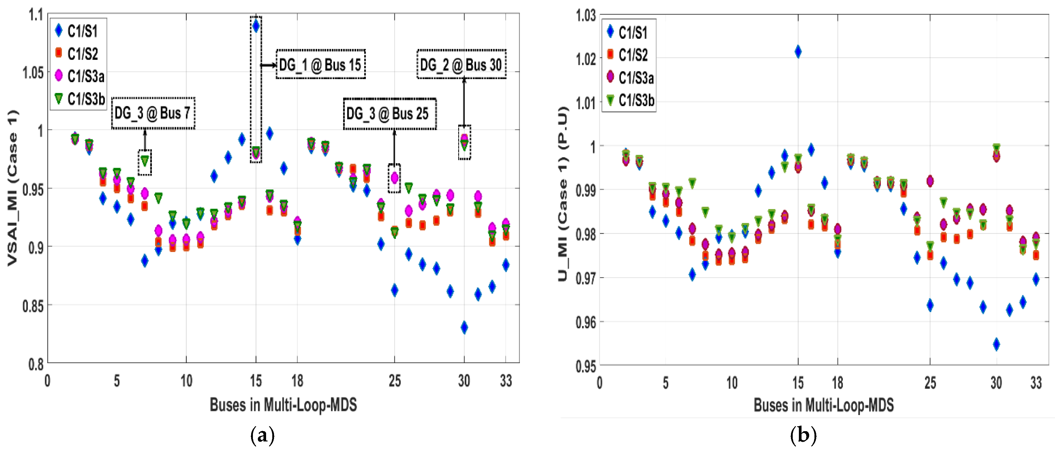
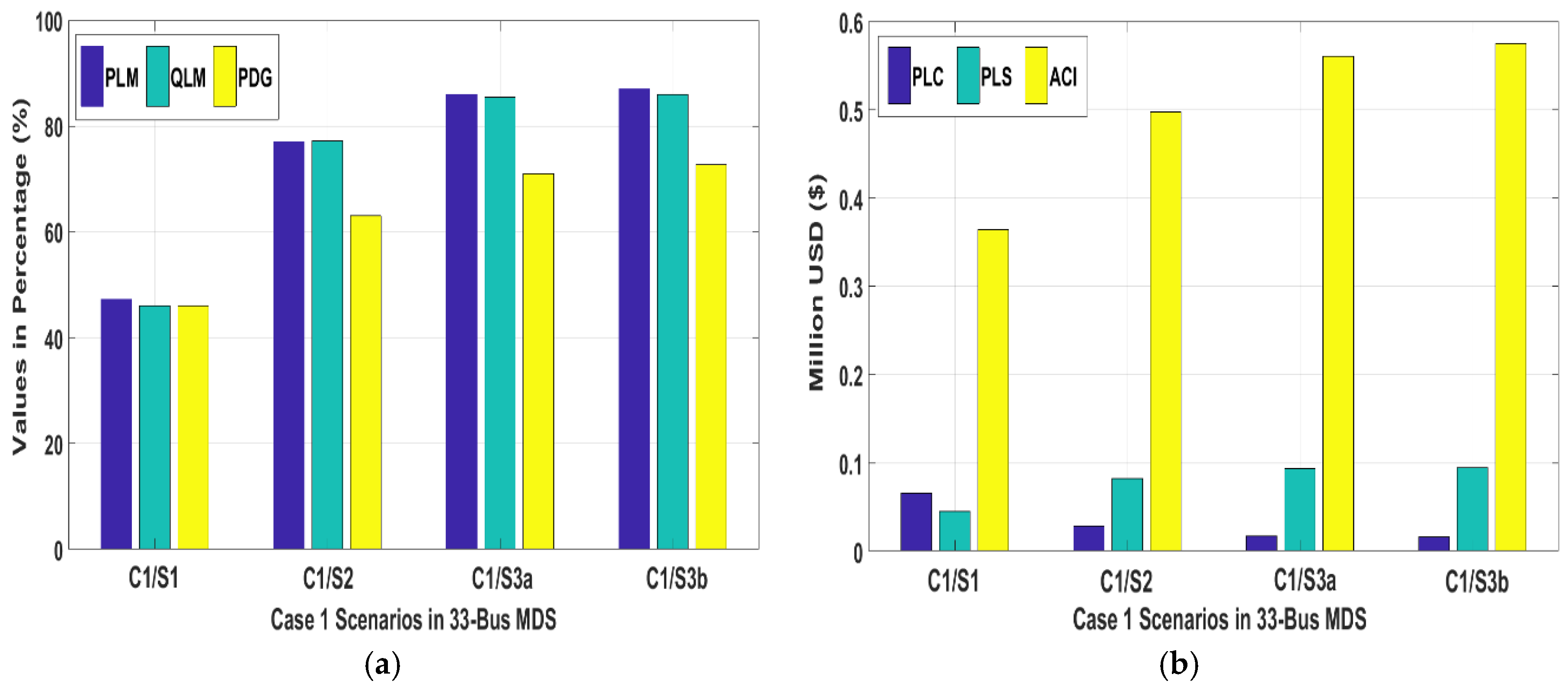
5.1.2. Evaluation of Case 1 (C1): DG Sitting and Sizing for Voltage-Maximization (U_Max)

The case 1 (C1) corresponds to the VSAI-LMC based planning approaches. The only difference is the selection of either of proposed VSAIs, as derived in Section 2.2 and Section 2.3. In addition to C1, the evaluation of each case is arranged in accordance with a various number of scenarios (S#) in accordance with computation procedures for both PA1 and PA2, for ease of understanding the “validation of concept.” The case and respective scenario number are arranged as (C#/S#).

Following base case 0a, the DG_1 is placed in accordance with the Step 5 of computation procedure of PA1. This gives the first scenario of base case 1 and is shown as C1/S1. Each DG, in this case, is operating at pf = 0.9 with the margin of ±2.5%, primarily aiming at U-Max along with other objectives. According to Step 6 (of PA1), DG_2 is placed and the respective scenario fulfilling the conditions mentioned in Step 7 (of PA1) is designated as C1/S2. In accordance with Step 8 (of PA1), DG_3 is placed and associated scenario fulfilling conditions in Steps 9 and 10 (of PA1) is designated as C1/S3a. Likewise, the simultaneous sitting of two DGs followed by Steps 1–6 of PA2 and respective scenario fulfilling conditions of Steps 7–10 is designated as C1/S3b.

The VSAI trends and associated U-profiles from the perspective of VSAI_MI-LMC and VSAI_MA-LMC of all scenarios of C1 are illustrated in Figure 7a,b and Figure 8a,b. In Figure 7a, VSAI trend based on idealistic MDS model is designated with VSAI_MI and U-profile is indicated with U_MI in Figure 7b. Likewise, in Figure 8a, VSAI trend based on actual MDS model is designated with VSAI_MA and U-profile is indicated with U_MA in Figure 8b. Evaluation of results pertaining to C1 with all associated scenarios is presented in

Table 2. Results of proposed planning approach under Case 1 (33-bus-MDS) aim at U_Max.

C#/S#:	DG (Size, Site, No.)	VSAI_MI/VSAI_MA	U_MI (P.U)/U_MA (P.U)	P_L (KW)/PLM (%)	Q_L (KVAR)/QLM (%)	PLC(M-$)/PLS (M-$)	PDG (%)/RSS (P + jQ)	ACI (M-$)
C1/S1	(2013,15,1) DG_1@15	1.09@15/1.001@15	1.022@15/1.002@15	125/47.2%	89/46%	0.0657/0.045	46.1%/2377 + j1757	0.3638
	DG_2 (Site)	0.955@30/0.9618@30	0.9550@30/0.9617@30
C1/S2	(971,15,1) DG_1@15	0.981@15/0.956@15	0.9952@15/0.9854@15	54.7/77%	37.5/77.25%	0.02875/0.0822	63%/1680 + j1498	0.4976
	(1783,30,2) DG_2@30	0.955@30/0.9618@30	0.9979@30/0.9844@30
	DG_3 (Site)	0.9130@25/0.9220@25	0.9749@25/0.9805@25
C1/S3a	(894.6,15,1) DG_1@15	0.9800@15/0.9551@15	0.9950@15/0.9860@15	33.2/86%	23.94/85.5%	0.01746/0.09345	71%/1400 + j1322	0.5607
	(1386,30,2) DG_2@30	0.9995@30/0.9780@30	0.9980@30/0.9880@30
	(822.6,25,3) DG_3@25	0.9591@25/0.9220@25	0.9920@25/0.9870@25
C1/S3b	(832.6,15,1) DG_1@15	0.9820@15/0.9580@15	0.9970@15/0.9900@15	30.85/87%	23.29/85.9%	0.0162/0.0947	72.8%/1308 + j1321	0.5750
	(1602,30,2) DG_2@30	0.9880@30/0.9540@30	0.9994@30/0.9880@30
	(745.1,7,3) DG_3@7	0.9742@7/0.9616@7	0.9940@7/0.9890@7

Size if shown in KVA @ pf = 0.9 ± 2.5%, Site is shown by @ bus No. in TDS, P + jQ = (KW) + j(KVAR), M$: Million USD.

.

It is observed that LMC is compromised during Step 5 (C1/S1) aiming at DG_1 siting and sizing. During Steps 6 and 7 (C1/S2), LMC is nearly achieved with DG_2 (siting and sizing) across TB (including TS4) and the respective value of loop currents (I_Lp1) is minimized to an insignificant numerical value. The difference of values in ΔU_Ref (obtained from equivalent ATP/EMTP and Matlab model), ΔU_MI and ΔU_MA, across bus 18 and bus 33, are (0.0001, 0.0011 and 0.0010). During Steps 8 and 9 (C1/S3a), bus 25 is the weakest bus, doubly fed by two ends and is a potential candidate for DG_3 (sitting and sizing). C1/S3a aims at LMC achievement across TB (including TS5) with I_Lp2 is minimized to a minor numerical value. The values in ΔU_Ref, ΔU_MI and ΔU_MA after DG_3, across buses 18–33 and 25–29, are (0.0000, 0.0004, 0.0001) and (0.0010, 0.0064, 0.0013). Moreover, it is also observed that VSAI_MI based values results in more deviation as compare to VSAI_MA based numerical values.

During PA2 or C1/S3b, the simultaneous DG sitting and sizing case results in better results. The LMC values across TBs (TS4 and TS5) and the respective value of loop currents (I_Lp1 and I_Lp2) are aimed to be retained at lower numerical values. The values in ΔU_Ref, ΔU_MI and ΔU_MA, across buses 18–33 and 25–29, are (0.0010, 0.0010, 0.0009) and (0.0009, 0.0050, 0.0003), respectively. It is also found that like C1/S3a, VSAI_MI based planning approach results in more deviation in numerical values, as compared to its actual MDS based counterpart (VSAI_MA centric). Hence, the numerical results of VSAI_MA-LMC based planning can be considered more credible.

The respective VSAI trends and associated U-profile have already been shown in Figure 7a,b and Figure 8a,b. The comparative analysis of case C1, with all relevant scenarios, has been illustrated in Figure 9a,b and covers all the performance evaluation indicators (PEIs) as mentioned in Section 4.4. It is observed in Figure 9a that a significant PLM and QLM were achieved with optimal PDG with multiple (three) DG sitting and sizing (in both C1/S3a and C1/S3b). Similarly, Figure 9b shows that a significant reduction was observed in terms of PLC and a high margin in PLS was achieved with optimal sitting and sizing of three DGs with respective planning approaches, as illustrated by C1/S3a and C1/S3b. However, ACI increases with an increase in DG size. It is worth mentioning that the cost in terms of ACI can surpass in a trade-off solution if a better performance evaluation is achieved. Moreover, PLS across load growth can justify the employment of multiple DG sitting and sizing in MDS and this impact will be addressed in our future work.

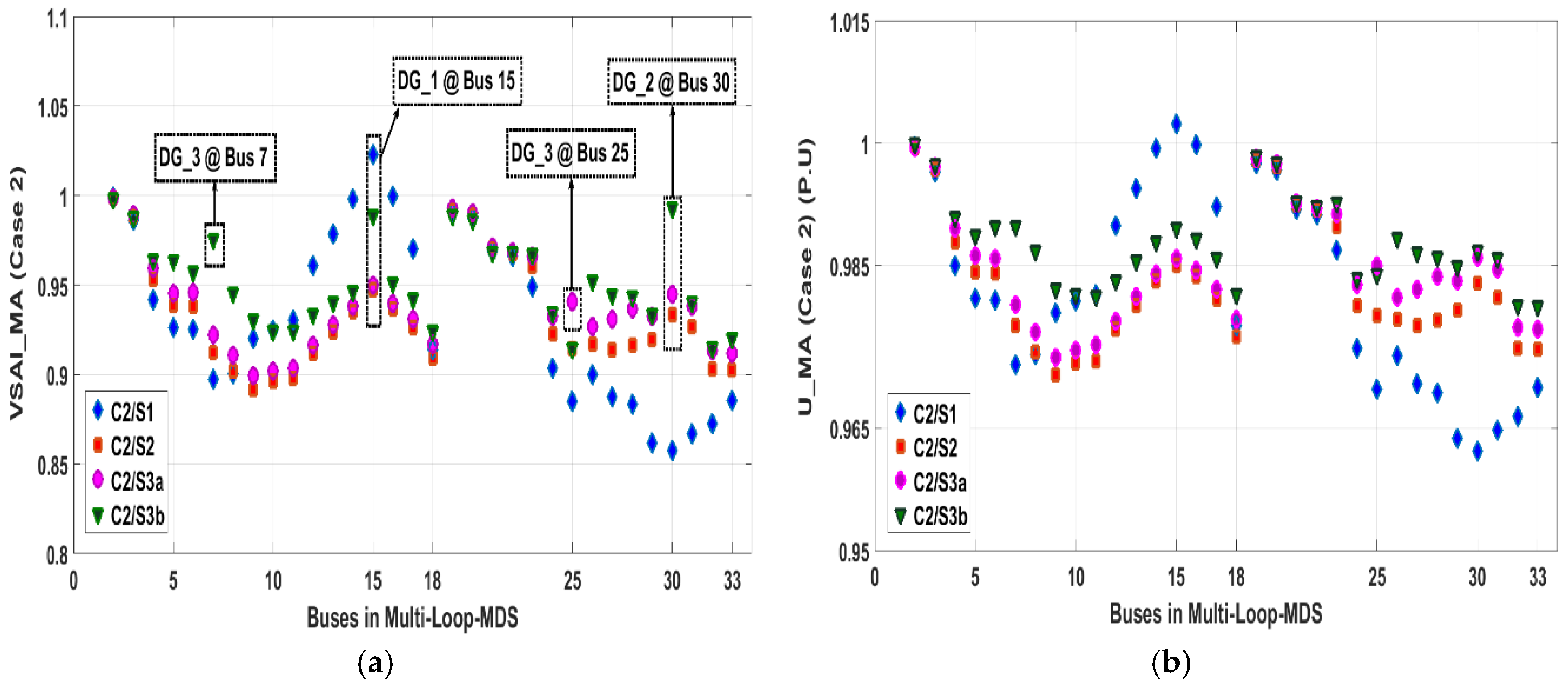
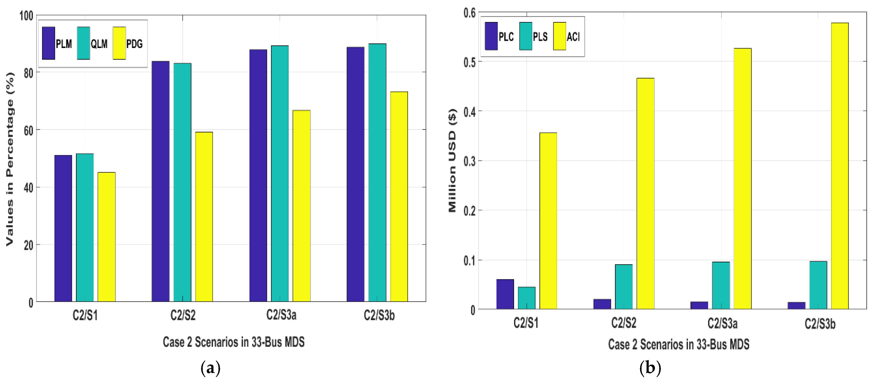
5.1.3. Evaluation of Case 2 (C2): DG Sitting and Sizing for Loss-Minimization (L_Min)

The evaluation procedure presented in Section 5.1.2 is repeated again for the proposed planning approach in terms of case 2 (C2) and mainly aims at L_Min besides other objectives attainment. The only core difference among C1 and C2 consists of DGs operating at respective pf, which is equal to that of TDS. The pf considered in C2 is 0.85 lagging with a ±2.5% variation, which in-terms of load indicate active and reactive power absorption and shows the capability of injecting both (active and reactive) powers in TDS from DG viewpoint.

VSAI trends and associated U-profiles from the perspective of each planning approach variants in-terms of respective scenarios of C2, are illustrated in Figure 10a,b and Figure 11a,b. The evaluation of results pertaining to C2 with all associated scenarios is presented in

Table 3. Results of proposed planning approach under Case 2 (33-bus-MDS) aim at L_Min.

C#/S#:	DG (Size, Site, No.)	VSAI_MI/VSAI_MA	U_MI (P.U)/U_MA (P.U)	P_L (KW)/PLM (%)	Q_L (KVAR)/QLM (%)	PLC(M-$)/PLS (M-$)	PDG (%)/RSS (P + jQ)	ACI (M-$)
C2/S1	(1969.6,15,1) DG_1@15	1.087@15/1.023@15	1.021@15/1.003@15	115.6/51.13%	79.7/51.6%	0.0608/0.0501	45.1%/2505 + j1604	0.356
	DG_2 (Site)	0.8300@30/0.8580@30	0.9549@30/0.9620@30
C2/S2	(950,15,1) DG_1@15	0.9728@15/0.9470@15	0.9935@15/0.9851@15	38.3/84%	28.1/83%	0.0201/0.0908	59%/1970 + j1277	0.467
	(1633,30,2) DG_2@30	0.9838@30/0.9333@30	0.9956@30/0.9830@30
	DG_3 (Site)	0.9139@25/0.9167@25	0.9732@25/0.9786@25
C2/S3a	(877,15,1) DG_1@15	0.9729@15/0.9501@15	0.9940@15/0.9860@15	28.8/87.9%	17.81/89.2%	0.01512/0.09600	67%/1703 + j1117	0.526
	(1310,30,2) DG_2@30	0.9774@30/0.9449@30	0.9950@30/0.9860@30
	(725,25,3) DG_3@25	0.9560@25/0.9410@25	0.9890@25/0.9850@25
C2/S3b	(828.3,15,1) DG_1@15	0.9890@15/0.9640@15	0.9930@15/0.9898@15	26.7/88.7%	16.75/89.8%	0.0140/0.0969	73.24%/1474 + j975	0.5782
	(1644,30,2) DG_2@30	0.9930@30/0.9701@30	0.9993@30/0.9869@30
	(727.8,7,3) DG_3@7	0.9755@7/0.9600@7	0.9899@7/0.9902@7

Size if shown in KVA @ pf = 0.85 ± 2.5%, Site is shown by @ bus No. in TDS, P + jQ = (KW) + j(KVAR), M$: Million USD.

.

From the perspective of a VSAI-LMC based planning approach during Steps 6 and 7 (C2/S2), LMC is nearly achieved for DG_2 (sitting and sizing) in the same fashion as mentioned in C1/S2. The I_Lp1 is minimized from the reference of difference in voltage across TB. The values (for C2/S2) in ΔU_Ref, ΔU_MI and ΔU_MA, across bus 18 and bus 33, are (0.0002, 0.0012 and 0.0010). During Step 8 and 9 (C2/S3a), after DG_3 (sitting and sizing) aiming at LMC achievement across TB (including TS5) with I_Lp2 is also minimized. The values in ΔU_Ref, ΔU_MI and ΔU_MA after DG_3, across buses 18–33 and 25–29, are (0.0000, 0.0006, 0.0005) and (0.0009, 0.0061, 0.0018).

In C2/S3b, the simultaneous DG sitting and sizing case achieved better results. The LMC across TBs (TS4 and TS5) with loop currents (I_Lp1 and I_Lp2) is achieved in terms of the negligible voltage difference. The values in ΔU_Ref, ΔU_MI and ΔU_MA, across buses 18–33 and 25–29, are (0.0002, 0.0011, 0.0010) and (0.0010, 0.0055, 0.0010). It was also found that the VSAI_MI based planning approach results in more deviation in numerical values, as compared to VSAI_MA centric approach.

The comparative analysis of C2 with all relevant scenarios are illustrated in Figure 12a,b and covers all the performance evaluation indicators (PEIs) (as aforementioned in Section 4.4). It is worth mentioning that an increase in reactive power support from DG results in effective L_Min as shown in C2 and U_profile achieved is nearly identical to those achieved in C1.

It can be observed in Figure 12a that a significant PLM and QLM were achieved with optimal PDG with multiple (three) DG sitting and sizing, in comparison with case 1 (mentioned in Figure 9a). Similarly, Figure 12b shows that a significant reduction was observed in terms of PLC and high margin in PLS have achieved with three DGs placement, as compare to C1 (mentioned in Figure 9b).

It is worth mentioning that more reactive power support is provided in C2 as compared to C1. It is important to note that ACI values in C2/S1, C2/S2 and C2/S3, are less in comparison with C1/S1, C1/S2 and C1/S3. The ACI values in C2/S3b show exception in comparison with C1/S3b. The reason includes high DG penetration that results in greater achieved (ACI) value. Like C1, in C2, increased ACI values can be justified with improved performance evaluation.

5.2. 69-Bus Mesh Distribution System

5.2.1. Evaluation of Base Case 0b (No DG)

The usefulness and assessment of the enhanced VSAI-LMC based planning approach will be further verified and explained on the 69-bus TDS (shown in Figure 5b), as a benchmark analysis. In order to retain discussion to the point, numerical results of only PA1 will be illustrated. According to the computation procedure of PA1 in Section 4.1, Steps 1–4 indicate the case with no DG residing in TDS. The base case in 69-bus TDS is indicated with “base case 0b” to avoid any confusion. The designation of variables in this sub-sub-section have retained in accordance with Section 5.1.1, in order to retain the symmetry of concept synchronization.

The only difference from the TDS perspective is the selection of TSs (TS3 and TS5), which convert RDS to a multiple loop topology based MDS. The TS3 resides within the TB between buses 15 and 46. Likewise, TS5 resides within the TB joining buses 27 and 65. The TS3 and TS5 in 69-bus TBS are closed to achieve multiple-loop configured MDS. The numerical results in the form of relevant VSI/VSAI trends and U-profiles of RDS, LDS and MDS are shown in Figure 13a,b.

In Figure 13a, it is noticed that bus 65 is the weakest bus according to VSI_R [17]. However, in MDS, bus 61 is the weakest bus according to VSI_L [37,38], VSAI_MI and VSAI_MA. It is observed in Figure 13b that the U-profile at various buses is below the minimum acceptable voltage limit, (0.95 P.U). The findings of the proposed approach with no DG are illustrated in

Table 4. Results of proposed planning approach without DG units (Base Case 0b).

Parameters	RDS	LDS (TS5)	MDS (TS3, TS5)	Weakest Bus
P_Load (KW)	3802.58	3802.58	3802.58	-
Q_Load (KVAR)	2692.9	2692.9	2692.9	-
P_L (KW)	224.98	260.74	244.69	-
Q_L (KVAR)	102.11	147.92	126.90	-
VSI_R [17]	0.6843 @ Bus 65	-	-	U_R = 0.9089@ Bus 65
VSI_L (Equation (1))	-	0.7170 @ Bus61	0.7200 @ Bus 61	Bus 61
VSAI_MI (Equation (15))	-	-	0.7104 @ Bus 61	Bus 61
VSAI_MA (Equation (24))	-	-	0.7220 @ Bus 61	Bus 61
U_L (Equation (2))	-	0.9190 @ Bus61	0.9210 @ Bus 61	Bus 61
U_MI (Equation (16))	-	-	0.9000 @ Bus 61	Bus 61
U_MA (Equation (25))	-	-	0.9220 @ Bus 61	Bus 61
PLC (Million-$) (Equation (36a))	0.11825	0.137045	0.12861	-

.

5.2.2. Evaluation under Case 3 (C3): DG Sitting and Sizing for Voltage-Maximization (U_Max)

The case 3 (C3) corresponds to the VSAI -LMC based planning approaches, considering 69-bus TDS. Subsequent to base case 0b, the DG_1 is placed in accordance with the Step 5 of computation procedure of PA1. This gives the first scenario of C3 and is shown as C3/S1. Each DG in this case is operating at pf = 0.9 ± 2.5%, primarily aiming at U-Max along with achieving other objectives. According to Steps 6 and 7 (of PA1), DG_2 (sitting and sizing) is designated as C3/S2. In Steps 8 and 9 (of PA1), DG_3 sitting and sizing with associated conditions met, are designated by C3/S3. The VSAI trends and associated U-profiles from the perspective of VSAI_MI-LMC and VSAI_MA-LMC of all scenarios of case 2, are illustrated in Figure 14a,b and Figure 15a,b.

Following DG_1 placement (Steps 1–5), in Steps 6 and 7 (C3/S2) of PA1, initial LMC condition is achieved with DG_2 (sitting and sizing) such that I_Lp1 (TB between buses 27 and 65, with TS5) is minimized from the reference of voltage difference. The values ΔU_Ref, ΔU_MI and ΔU_MA, across bus 27 and bus 65, are (0.0001, 0.0002 and 0.0000). During Steps 8 and 9 of PA1 (and designated with C3/S3), improved LMC condition, besides I_Lp2 (across TB including TS5), is achieved across other TB (between buses 15 and 46, with TS3) in-terms of minimizing I_Lp2. The evaluated values in-terms of ΔU_Ref, ΔU_MI and ΔU_MA after DG_3 sitting and sizing, across buses 27–65 (TS5) and 15–46 (TS3), are (0.0001, 0.0029, 0.0002) and (0.0003, 0.0007, 0.0003).

The trend in terms of deviation in voltage based numerical values is observed more in VSAI_MI, in comparison with the VSAI_MA based planning approach. The numerical values achieved in the VSAI trend and U_profile in VSAI_MI-LMC based planning approach shows highest upper metric limits in C3/S1, whereas its more stable in other two scenarios, whereas attained respective results are more stable in VSAI_MA-LMC based approach across all scenarios or C3. Hence, the credibility of the VSAI_MA-LMC based planning approach is validated and supported with respective results.

Evaluation of results pertaining to C3 with all associated scenarios is presented in

Table 5. Results of proposed planning approach under Case 3 (69-bus-MDS) aim at U_Max.

C#/S#:	DG (Size, Site, No.)	VSAI_MI/VSAI_MA	U_MI (P.U)/U_MA (P.U)	P_L (KW)/PLM (%)	Q_L (KVAR)/QLM (%)	PLC(M-$)/PLS (M-$)	PDG (%)/RSS (P + jQ)	ACI (M-$)
C3/S1	(2578,61,1) DG_1@61	1.070@61/1.004@61	1.017@61/1.001@61	59.1/75.84%	33.4/73.7%	0.0311/0.0872	55.34%/1884 + j2012	0.4659
	DG_2 (Site)	0.9520@21/0.9604@21	0.9877@21/0.9899@21
C3/S2	(2326,61,1) DG_1@61	1.054@61/1.004@61	1.013@61/1.001@61	40.4/83.5%	27.51/78.2%	0.02122/0.09804	61.9%/1616 + j1873	0.521
	(557,21,2) DG_2@21	1.027@21/1.000@21	1.007@21/1.000@21
	DG_3 (Site)	0.9670@12/0.9770@12	0.9920@12/0.9940@12
C3/S3 or (C3/S3a)	(2284,61,1) DG_1@61	1.050@61/1.027@61	1.013@61/1.0008@61	22.35/90.9%	13.3/89.53%	0.0175/0.1065	68.6%/1343 + j1716	0.57719
	(442.9,21,2) DG_2@21	1.019@21/1.0000@21	1.005@21/1.0000@21
	(467.5,12,3) DG_3@12	1.0036@12/1.0025@12	0.9951@12/0.9985@12

Size if shown in KVA @ pf = 0.9 ± 2.5%, Site is shown by @ bus No. in TDS, P + jQ = (KW) + j(KVAR), M-$: Million USD.

. The comparative analysis aim at case C3 with all relevant scenarios is illustrated with PEIs in Figure 16a,b. It is observed in Figure 16a that optimal PDG (three DGs) sitting and sizing results in a noteworthy PLM and QLM by percentage. Similarly, the results in Figure 16b justified the reduction in PLC and an increase in the PLS margin. The increased ACI can be justified on the basis of a better performance evaluation, achieved in C3.

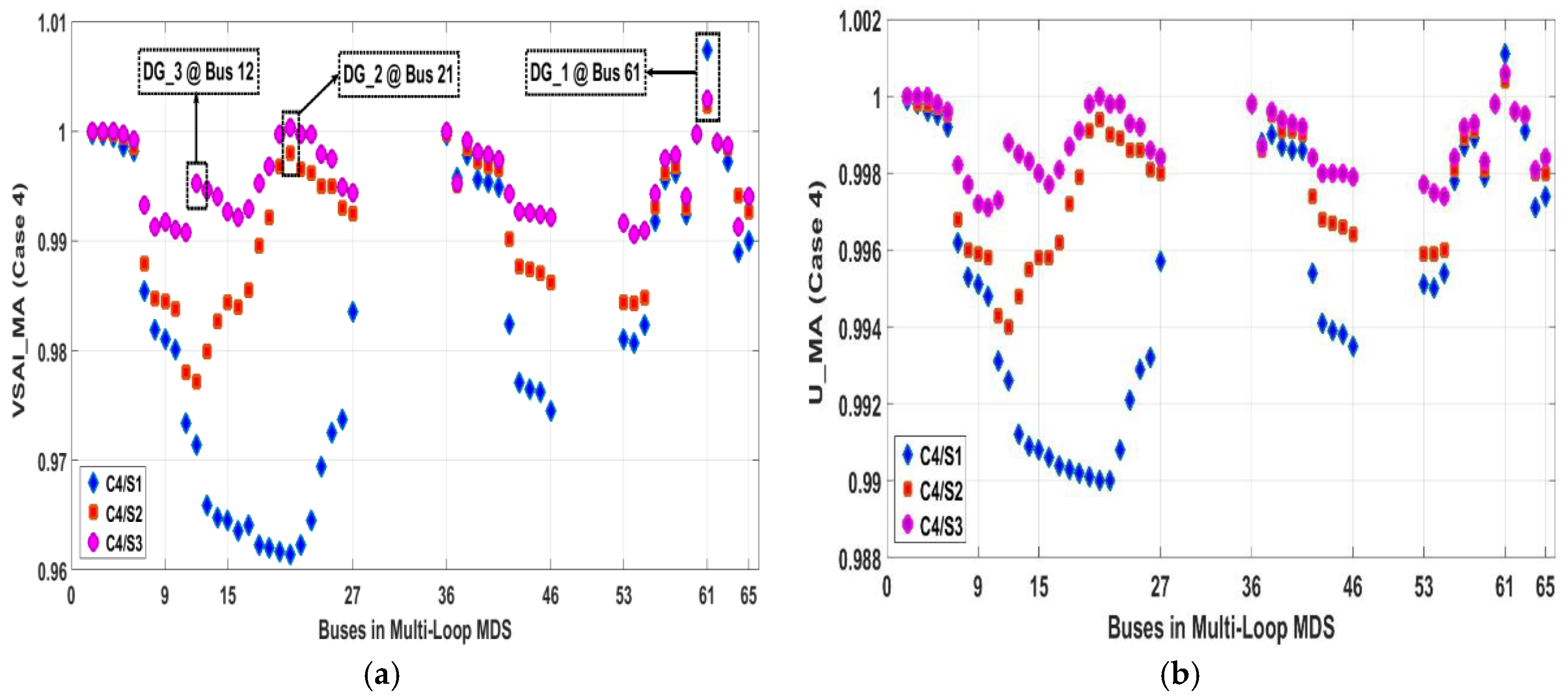
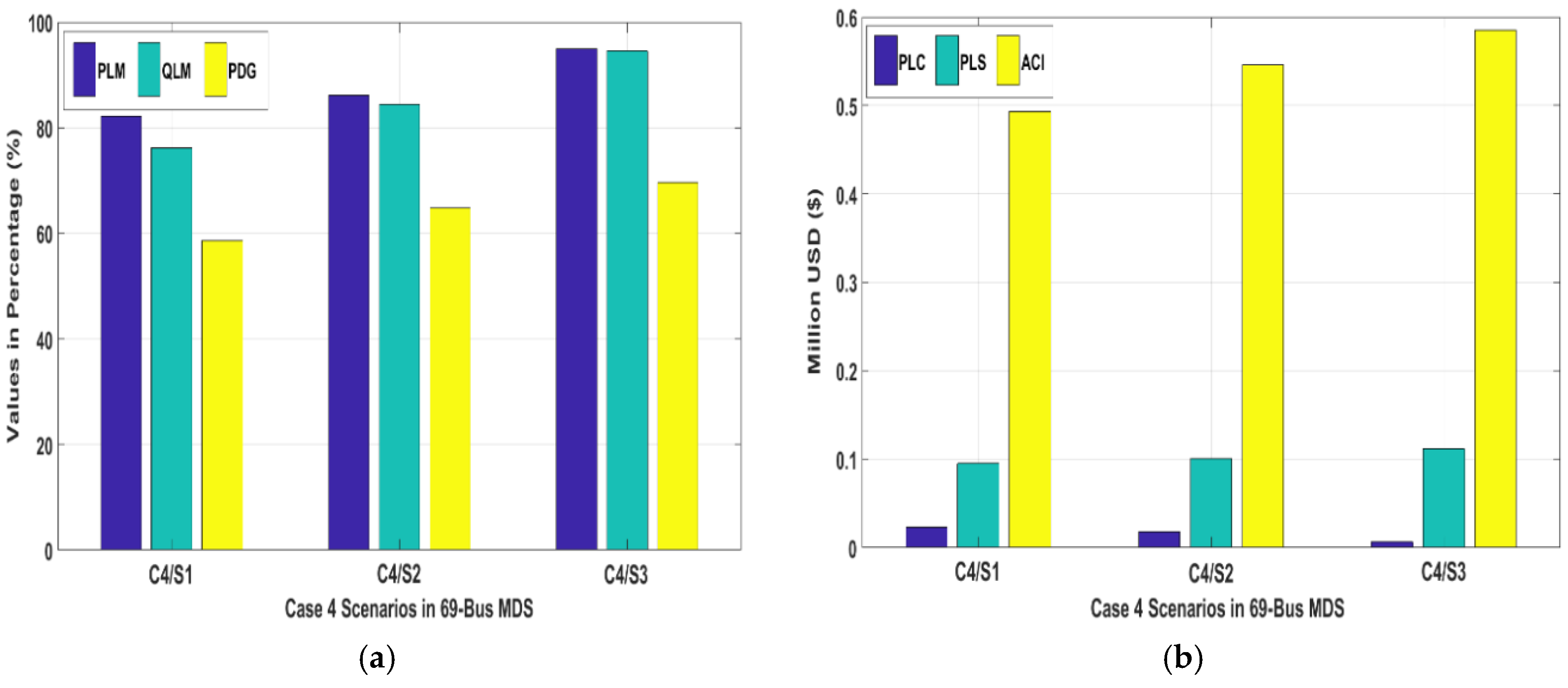
5.2.3. Evaluation under Case 4 (C4): DG Sitting and Sizing for Loss-Minimization (L_Min)

The respective C4 aims at L_min and pf considered in C4 is 0.82 ± 2.5% lagging. The VSAI_MI-LMC and VSAI_MA-LMC trends and associated U-profiles, from the viewpoint of each C3 scenarios is distinctively illustrated in Figure 17a,b and Figure 18a,b.

Following Steps (1–5) for DG_1 placement via planning approach, during Steps 6 and 7 (C4/S2), the nearly ideal LMC is achieved across TS5 with minimizing I_LP1 to almost zero with DG_2 placement. The values (for C4/S2) in ΔU_Ref, ΔU_MI and ΔU_MA, across bus 27 and bus 65, are (0.00001, 0.000015 and 0.00001).

After DG_3 (sitting and sizing) employment during Steps 8 and 9 (C4/S3), LMC is achieved with reducing loop currents (I_LP1 and I_LP2) across both TS5 (buses 27 and 65) and TS3 (buses 15 and 46). The respective voltage difference values (for C4/S2) in ΔU_Ref, ΔU_MI and ΔU_MA, across TS5 is (0.0001, 0.00001 and 0.00012) and across TS3 is (0.0001, 0.0005 and 0.0001).

Evaluation of results pertaining to C4 with all associated scenarios is presented in

Table 6. Results of proposed planning approach under Case 4 (69-bus-MDS) aim at L_Min.

C#/S#:	DG (Size, Site, No.)	VSAI_MI/VSAI_MA	U_MI (P.U)/U_MA (P.U)	P_L (KW)/PLM (%)	Q_L (KVAR)/QLM (%)	PLC(M-$)/PLS (M-$)	PDG (%)/RSS (P + jQ)	ACI (M-$)
C4/S1	(2730,61,1) DG_1@61	1.071@61/1.0004@61	1.018@61/1.0004@61	43.58/82.2%	30.2/76.17%	0.02291/0.09536	58.6%/1950 + j1569	0.4933
	DG_2 (Site)	0.9530@21/0.9614@21	0.9880@21/0.9900@21
C4/S2	(2490,61,1) DG_1@61	1.0572@61/1.0023@61	1.014@61/1.00039@61	33.8/86.2%	19.804/84.4%	0.0178/0.10049	64.8%/1718 + j1413	0.5453
	(528,21,2) DG_2@21	1.0192@21/0.9979@21	1.005@21/0.9995@21
	DG_3 (Site)	0.9670@12/0.9770@12	0.9915@12/0.9940@12
C4/S3 or (C4/S3a)	(2444,61,1) DG_1@61	1.055@61/1.030@61	1.013@61/1.0006@61	12.26/95%	6.492/94.5%	0.006442/0.111839	72.88%/1413 + j1204	0.5853
	(440,21,2) DG_2@21	1.016@21/1.0003@21	1.005@21/1.000@21
	(512,12,3) DG_3@12	1.006@12/0.9953@12	1.004@12/0.999@12

Size if shown in KVA @ pf = 0.82 ± 2.5%, Site is shown by @ bus No. in TDS, P + jQ = (KW) + j(KVAR), M-$: Million USD.

. The comparative analysis of C4 with all relevant scenarios from the viewpoint of PEIs are illustrated in Figure 19a,b. It is also interesting to know that increase in reactive power support from DG have result in almost the same U_profile trend as achieved in C3.

It is observed in Table 6 that a significant PLM and QLM by percentage have been achieved with improved optimal PDG, in comparison with C3. From a comparison perspective of C1–C2 (33-Bus TDS), less PDG has observed in C3–C4 (69-Bus TDS). It is interesting to observe that 33-Bus TDS is a heavy loaded system as compare to 69-Bus-TDS on load distribution level.

Similarly, Table 6 shows that a substantial decrease is observed in-terms of PLC and improved PLS margin. The ACI trend in C4 has surpassed C3 across all scenarios. Although ACI is high, however, it can be justified with improved PEI results and cost to benefit analysis across load growth. Since load growth across planning horizon is out of the scope of this paper. In future, a multi-objective based trade-off solution across a load growth will be addressed in our future publications.

6. Comparison/Validation Analysis

6.1. Results Comparison with Existing Works

The proposed VSAI-LMC based planning approach aims at (multiple-loop configured) MDS is evaluated on 33-Bus and 69-Bus TDS and validated via comparative analysis of achieved results with the findings in the available literature. The comparison methods considered in this section include various techniques such as VSI centered approach in [18] for RDS (69-Bus), non-sorting-genetic algorithm (NSGA-II) based planning approach in [29] for LDS (69-Bus). Moreover, sensitivity based approach [31] for MDS (33-Bus), VSI-LMC centered approach in [38] for LDS (69-Bus) and iterative algorithm (IA) based approach in [43] for RDS (33 and 69-Bus), have been also considered in the comparative study. Since, most of these techniques are proposed for RDS and offer comparison from one or two perspectives. The main aim of this section is to offer a big picture of MDS centered technique via comparison on the basis of performance evaluation across various multiple PEIs, as aforementioned in previous sections.

6.1.1. Comparison of Numerical Results with 33 Bus based Test Distribution System

The numerical results of proposed approach obtained from case 1 (C1) have been evaluated on 33 bus MDS considering four scenarios. The C1 corresponds to the U_max case, where all the DGs in C1 are operating at pf = 0.9 ± 2.5% lagging. The achieved results have compared with sensitivity based approach reported in Reference [31] considering 33-bus MDS. The comparison of results has been illustrated in

Table 7. Comparisons of results with various scenarios of Case 1 for 33-Bus test system (DG @ pf = 0.90 ± 2.5%).

Performance Evaluation Indicators (PEIs)	[31]	[31]	C1/S1	C1/S2	C1/S3a	C1/S3b
DG Size (KVA)@ DG Site (Bus#)	2706.7@6	2074.56@6 615.25@15	2013@15	971@15 1783@30	894.6@15 1386@30 822.6@25	832.6@15 1602@30 745.1@7
VSAI_MA@Bus-Min	-	-	0.9618@30	0.9110@33	0.9220@33	0.9170@33
U_MA@Bus (P.U)	0.98279	0.97567	0.9617@30	0.9770@33	0.9800@33	0.9782@33
P_L (KW)	117.88	65.8435	125	54.7	33.20	30.85
PLM (%)	44.14	68.8	47.2	77	86	87
Q_L (KVAR)	90.454	51.94	89	37.5	23.94	23.29
QLM (%)	36.75	63.7	46	77.25	85.5	85.9
PLC (Million-$)	0.062	0.03461	0.0657	0.02875	0.01746	0.0162
PLS (Million-$)	0.049	0.07629	0.0450	0.0822	0.09345	0.0947
DG Capacity (KVA)	2706.7	2689.81	2013	2754	3103.2	3179.7
PDG (%)	61.95%	61.56	46.1	63	71	72.8
RSS (KW + j KVAR)	256.43 + j 321.01	1347.9 + j 836.34	2377 + j 1757	1680 + j 1498	1400 + j 1322	1308 + j 1321
ACI (Million-$)	-	-	0.3638	0.4976	0.5607	0.5750

Note: The achieved results that outperformed compared works are shown in bold text.

. It is important to note via performance evaluation proposed approach that C1/S3b have resulted in significant power losses (P_L and Q_L) minimization, reduction in PLC, increase in PLS and improved PDG and satisfactory release (relief) in substation capacity (RSS). C1/S3b outperforms other scenarios across the maximum number of PEIs. C1/S3a outperforms other scenarios only from the viewpoint of VSAI trend and associated voltage profile.

The numerical results in-terms of C2 are evaluated on 33 bus MDS considering four scenarios in the same way as C1. The C2 corresponds to L_Min case, where all the DGs are operating at pf = 0.85 ± 2.5% lagging. The attained results are compared with iterative algorithm based approach reported in [43] and conducted on 33-bus RDS, where the comparison of results has been illustrated in

Table 8. Comparisons of results with various scenarios of Case 2 for 33-Bus test system (DG @ pf = 0.85 ± 2.5%).

Performance Evaluation Indicators (PEIs)	[43]	[43]	C2/S1	C2/S2	C2/S3a	C2/S3b
DG Size (KVA)@ DG Site (Bus#)	2118@6, 1059@30,	1059@6 768@14 1059@30	1969.6@15	950@15 1633@30	877@15 1310@30 725@25	828.3@15 1644@30 727.8@7
VSAI_MA@Bus-Min	-	-	0.8580@30	0.9167@33	0.9121@33	0.9221@33
U_MA@Bus (P.U)	-	-	0.9620@30	0.9750@18	0.9777@33	0.9805@33
P_L (KW)	44.84	23.05	115.6	38.3	28.8	26.7
PLM (%)	78.75	89.1	51.13	84	87.9	88.7
Q_L (KVAR)	-	-	79.7	28.1	17.81	16.75
QLM (%)	-	-	51.6	83	89.2	89.8
PLC (Million-$)	-	-	0.0608	0.0201	0.01512	0.0140
PLS (Million-$)	-	-	0.0501	0.0908	0.09600	0.0969
DG Capacity (KVA)	3177	2886	1969.6	2583	2912	3200
PDG (%)	72.71	66.1	45.1	59	67	73.24
RSS (KW + j KVAR)	-	-	2505 + j 1604	1970 + j 1277	1703 + j 1117	1474 + j 975
ACI (Million-$)	-	-	0.356	0.467	0.526	0.5782

Note: The achieved results that outperformed compared works are shown in bold text.

. It is noteworthy via performance evaluation that C2/3b has outperformed all other scenarios and compared works from the perspective of all mentioned PEIs as shown in Table 8. It is also interesting to know that a significant relief in substation power (RSS) has been achieved in a reactive component. Reason being, the multiple DGs in C2 have resulted in improved reactive power support and voltage stabilization, which is comparable with C1. Therefore, comparison analysis in both Table 7 and Table 8 demonstrates the effectiveness of the proposed method from the viewpoint of 33-Bus MDS. It is observed that ACI in both C1 and C2 have resulted in high numerical values. However, improved results in PEIs justify high ACI values.

6.1.2. Comparison of 69 Bus Test System Results with the Existing Research Works

The numerical results in the form of C3 have been evaluated for 69-bus MDS and constitute three scenarios. Since the test system serves as a benchmark analysis. Hence, for the proof of concept, only PA1 has been considered in this study. The C3 corresponds to a case, which aims at U_max and all the associated DGs are operating at pf = 0.9 ± 2.5% lagging (capable of injecting both active and reactive powers). The achieved results have compared with the VSI-based approach designed specifically for RDS [18]. Although there are other works available that considers DG operating at various power factors and comparison of PA1 with employment of DGs operating at pf = 0.9 ± 2.5%, may not be justified. Also, different pf can be considered in the proposed approach and this subject is out of the scope of this paper. Hence, the comparison among proposed and [18] for validation, is conducted for C3 considering DGs operating at pf = 0.9 ± 2.5%. The attained results have compared across various PEIs as illustrated in

Table 9. Comparisons of results with various scenarios of Case 3 for 69-Bus test system (DG @ pf = 0.90 ± 2.5%).

Performance Evaluation Indicators (PEIs)	[18]	C3/S1	C3/S2	C3/S3
DG Size (KVA)@ DG Site (Bus#)	2220@61	2578@61	2326@61 557@21	2284@61 442.9@21 467.5@12
VSAI_MA@Bus-Min	0.86585@26	0.9604@21	0.9770@12	0.9900@46
U_MA@Bus (P.U)	0.97273@26	0.9899@21	0.9940@12	0.9973@46
P_L (KW)	27.9	59.1	40.4	22.35
PLM (%)	16.4245	75.84	83.5	90.9
Q_L (KVAR)	0.86585@26	33.4	27.51	13.30
QLM (%)	0.97273@26	73.7	78.2	89.53
PLC (Million-$)	0.01466412	0.0311	0.02122	0.0175
PLS (Million-$)	0.10362	0.0872	0.09804	0.1065
DG Capacity (KVA)	2220	2578	2883	3194.4
PDG (%)	47.64	55.35	61.9	68.6
RSS (KW + j KVAR)	-	1884 + j 2012	1616 + j 1873	1343 + j 1716
ACI (Million-$)	-	0.4659	0.521	0.55719

Note: The achieved results that outperformed compared works are shown in bold text.

. It is important to mention that the VSAI trends and associated voltage profile based on actual MDS have been considered due to the credibility of their respective values.

The numerical results aiming at 69-bus MDS for L_Min case correspond to C4, where all DGs are operating at optimal pf equal to that of load such as 0.82 ± 2.5%. The main aim is to reduce system losses in addition to other objectives. The achieved numerical results have been compared with the VSI-based approach designed for RDS [18], the NSGA-II based planning approach designed for LDS [29] and the VSI-LMC based integrated approach for LDS. The attained results are arranged and compared across various PEIs in a tabular form as shown in

Table 10. Comparisons of results with various scenarios of Case 4 for 69-Bus test system (DG @ pf = 0.82 ± 2.5%).

Performance Evaluation Indicators (PEIs)	[18]	[29]	[38]	C4/S1	C4/S2	C4/S3
DG Size (KVA)@ DG Site (Bus#)	2240@61	2147@61 590@22	2328@61 400@22	2730@61	2490@61 528@21	2444@61 440@21 512@21
VSAI_MA@ Bus-Min	0.8083@57	-	0.9620@27	0.9614@21	0.9770@12	0.9922@46
U_MA@ Bus (P.U)	0.954425@26	-	0.9903@65	0.9900@21	0.9940@12	0.9980@46
P_L (KW)	23.124	23.4	25.367	43.58	33.8	12.26
PLM (%)	87.75	91	90.27	82.2	86.2	95
Q_L (KVAR)	14.363	-	17.2607	30.2	19.804	6.942
QLM (%)	85.95	-	-	76.17	84.4	94.5
PLC (Million-$)	0.012154	0.012299	0.013333	0.02291	0.0178	0.006442
PLS (Million-$)	0.106054	-	0.104875	0.09536	0.10049	0.111839
DG Capacity (KVA)	2240	2737	2728	2730	3018	3396
PDG (%)	48.07	58.73	58.55	58.6	64.8	72.88
RSS (KW + j KVAR)	2010.1 + j 1394.4	-	1527.389 + j 2738.723	1950 + j 1569	1718 + j 1413	1413 + j 1204
ACI (Million-$)	-	-	0.493	0.4933	0.5453	0.5853

Note: The achieved results that outperformed compared works are shown in bold text.

. In C4, like all other cases, VSAI trends and associated voltage profile based on actual MDS have been considered from a comparison perspective due to the credibility of their respective values. It is worth noticing that, in comparison with other related research, the proposed PA1 allows three DG (siting and sizing) employment in MDS and leads to improved performance evaluation, which was limited in the current (available) literature.

The proposed VSAI-LMC based planning approach with two computation variants has been compared with the existing literature and the results are in close agreement, validating our proposed approach. Moreover, from the perspective of achieved numerical results, the performance evaluation indicates that the multiple-loop configured MDS outperforms RDS and LDS, as illustrated in 33-Bus (C1 and C2) and 69-Bus (C3 and C4) TDS. In addition to being a reliable choice, better numerical values under the performance measurement and evaluation, MDS shows itself to be a potential candidate for SDS under an SG environment. In future studies, MDS-related planning problems will be resolved under conflicting multiple-objective optimization, performance evaluation across load growth (from the perspective of planning horizon) and integrated medium voltage (MV)/ Low voltage (LV) distribution system under SG paradigm.

7. Conclusions

This paper presents an integrated VSAI-LMC based integrating planning approach that covers all aspects of the electrically equivalent MDS model and is employed for the layout (sitting and sizing) of numerous DG units in the MDS. The proposed integrated approach comprises of two parts—VSAI is applied for potential DG locations for sitting (with initial sizing) and loss minimalize condition (LMC) for maximum loss minimizations with optimal DG sizing. Initially, the paper offers detailed mathematical derivations (expressions) of two VSAI indices, one based on an ideal MDS model and the other based on actual MDS equivalent models. Later, mathematical expressions for loss minimalize condition (LMC) were derived based on an equivalent MDS model. The proposed VSAI-LMC approach was applied with two computation variants. The core goal of each computation variant is to access MDS evaluation under several performance indicators. Furthermore, a comprehensive detail regarding well-known performance evaluation indicators (PEIs) employed in various studies have also been presented. The proposed planning approach was applied and tested on two recognized test distribution systems (TDS), namely 33-Bus and 69-Bus. The attained results across four cases (two cases for each TDS) have been broadly compared across related research and the results, besides being in close agreement, have outperformed them in various aspects and thus validate our proposed VSAI-LMC integrated planning approach for MDS. Moreover, it can be inferred that multiple loop configured MDS is a suitable candidate for SDS under an SG environment. In future, improved performance evaluation versus cost (mainly ACI) will be evaluated across load growth and respective planning horizon along with the application of multiple-criteria (conflicting objectives) based optimization.

References

1. Rodriguez, A.A.; Ault, G.; Galloway, S. Multi-Objective planning of distributed energy resources: A review of the state-of-the-art. Renew. Sustain. Energy Rev. 2010, 14, 1353–1366. [Google Scholar] [CrossRef]
2. Fang, X.; Misra, S.; Xue, G.; Yang, D. Smart grid—The new and improved power grid: A survey. IEEE Commun. Surv. Tutor. 2012, 14, 944–980. [Google Scholar] [CrossRef]
3. Evangelopoulos, V.A. Optimal operation of smart distribution networks: A review of models, methods, and future research. Electr. Power Syst. Res. 2016, 140, 95–106. [Google Scholar] [CrossRef]
4. Sayed, M.A.; Takeshita, T. Line Loss Minimization in Isolated Substations and Multiple Loop Distribution Systems Using the UPFC 2014. IEEE Trans. Power Electron. 2014, 29, 5813–5822. [Google Scholar] [CrossRef]
5. Kim, J.C.; Cho, S.M.; Shin, H.S. Advanced Power Distribution System Configuration for Smart Grids. IEEE Trans. Smart Grid 2013, 4, 353–358. [Google Scholar] [CrossRef]
6. Kazmi, S.A.A.; Shahzad, M.K.; Khan, A.Z.; Shin, D.R. Smart Distribution Networks: A Review of Modern Distribution Concepts from Planning Perspectives. Energies 2017, 10, 501. [Google Scholar] [CrossRef]
7. Keane, A.; Ochoa, L.F.; Borges, C.L.T.; Ault, G.W.; Alarcon-Rodriguez, A.D.; Currie, R.; Pilo, F.; Dent, C.; Harrison, G.P. State-of-the-art techniques and challenges ahead for distributed generation planning and optimization. IEEE Trans. Power Syst. 2013, 28, 1493–1502. [Google Scholar] [CrossRef]
8. Kazmi, S.A.A.; Shahzad, M.K.; Shin, D.R. Multi-Objective Planning Techniques in Distribution Networks: A composite Review. Energies 2017, 10, 208. [Google Scholar] [CrossRef]
9. Ju, Y.; Wu, W.; Zhang, B.; Sun, H. Loop-analysis-based continuation power flow algorithm for distribution networks. IET Gen. Trans. Distrib. 2014, 8, 1284–1292. [Google Scholar] [CrossRef]
10. Jordehi, A.R. Allocation of distributed generation units in electric power systems: A review. Renew. Sustain. Energy Rev. 2015, 56, 893–905. [Google Scholar] [CrossRef]
11. Prakash, P.; Khatod, D.K. Optimal sizing and sitting techniques for distributed generation in distribution systems: A review. Renew. Sustain. Energy Rev. 2016, 57, 111–130. [Google Scholar] [CrossRef]
12. Sedghi, M.; Ahmadian, A.; Golkar, M.A. Assessment of optimization algorithms capability in distribution network planning: Review, comparison and modification techniques. Renew. Sustain. Energy Rev. 2016, 66, 415–434. [Google Scholar] [CrossRef]
13. Modarresi, J.; Gholipour, E.; Khodabakhshain, A. A comprehensive review of the voltage stability indices. Renew. Sustain. Energy Rev. 2016, 63, 1–12. [Google Scholar] [CrossRef]
14. Vita, V. Development of a decision-making algorithm for the optimum size and placement of distributed generation units in distribution network. Energies 2017, 10, 1433. [Google Scholar] [CrossRef]
15. Vita, V.; Alimardan, T.; Ekonomou, L. The impact of distributed generation in the distribution networks’ voltage profile and energy losses. In Proceedings of the 9th IEEE European Modelling Symposium on Mathematical Modelling and Computer Simulation, Madrid, Spain, 6–8 October 2015; pp. 260–265. [Google Scholar]
16. Hadjiionas, S.; Oikonomou, D.S.; Fotis, G.P.; Vita, V.; Ekonomou, L.; Pavlatos, C. Green field planning of distribution systems. In Proceedings of the 11th WSEAS International Conference on Automatic Control, Modelling and Simulation, Istanbul, Turkey, 30 May 30–1 June 2009; pp. 340–348. [Google Scholar]
17. Chakravorty, M.; Das, D. Voltage stability analysis of radial distribution networks. Int. J. Electr. Power Energy Syst. 2001, 23, 129–135. [Google Scholar] [CrossRef]
18. Murty, V.V.S.N.; Kumar, A. Optimal placement of DG in radial distribution systems based on new voltage stability index under load growth. Electr. Power Syst. Res. 2015, 69, 246–256. [Google Scholar] [CrossRef]
19. Quezada, V.M.; Abbad, J.R.; Roman, T.G.S. Assessment of energy distribution losses for increasing penetration of distributed generation. IEEE Trans. Power Syst. 2006, 21, 533–540. [Google Scholar]
20. Hung, D.Q.; Mithulananthan, N.; Bansal, R.C. Analytical strategies for renewable distributed generation integration considering energy loss minimization. Appl. Energy 2013, 105, 75–85. [Google Scholar] [CrossRef]
21. Hung, D.Q.; Mithulananthan, N. Loss reduction and loadability enhancement with DG: A dual-index analytical approach. Appl. Energy 2014, 115, 233–241. [Google Scholar] [CrossRef]
22. Aman, M.M.; Jasmon, G.B.; Mokhlis, H.; Bakar, A.H.A. Optimal placement and sizing of a DG based on a new power stability index and line losses. Int. J. Electr. Power Energy Syst. 2012, 43, 1296–1304. [Google Scholar] [CrossRef]
23. Kalambe, S.; Agnihotri, G. Loss minimization techniques used in distribution network: Bibliographic survey. Renew. Sustain. Energy Rev. 2014, 29, 184–200. [Google Scholar] [CrossRef]
24. Sultanaa, U.; Khairuddin, A.B.; Aman, M.M.; Mokhtara, A.S.; Zareen, N. A review of optimum DG placement based on minimization of power losses and voltage stability enhancement of distribution system. Renew. Sustain. Energy Rev. 2016, 63, 363–378. [Google Scholar] [CrossRef]
25. Viral, R.; Khatod, D.K. Optimal planning of distributed generation systems in distribution system: A review. Renew. Sustain. Energy Rev. 2012, 16, 5146–5165. [Google Scholar] [CrossRef]
26. Georgilakis, P.S.; Hatziargyriou, N.D. Optimal Distributed Generation Placement in Power Distribution Networks: Models, Methods, and Future Research. IEEE Trans. Power Syst. 2013, 28, 3420–3428. [Google Scholar] [CrossRef]
27. Georgilakis, P.S.; Hatziargyriou, N.D. A review of Power distribution planning in the modern power systems era: Models, methods, and future research. Electr. Power Syst. Res. 2015, 121, 89–100. [Google Scholar] [CrossRef]
28. Chen, T.H.; Huang, W.T.; Gu, J.C.; Pu, G.C.; Hsu, Y.F.; Guo, T.Y. Feasibility study of upgrading primary feeders from radial and open loop to normally closed-loop arrangement. IEEE Trans. Power Syst. 2004, 19, 1308–1316. [Google Scholar] [CrossRef]
29. Buayai, K.; Ongsaku, W.; Mithulananthan, N. Multi-objective micro-grid planning by NSGA-II in primary distribution system. Eur. Trans. Electr. Power 2011, 22, 170–187. [Google Scholar] [CrossRef]
30. Sharma, A.K.; Murthy, V.V.S.N. Analysis of Meshed Distribution Systems Considering Load models and Load growth Impact with Loops on System Performance. J. Inst. Eng. 2014, 95, 295–318. [Google Scholar]
31. Murthy, V.V.S.N.; Ashwani, K. Mesh distribution system analysis in presence of distributed generation with time varying load model. Int. J. Electr. Power Energy Syst. 2014, 62, 836–854. [Google Scholar] [CrossRef]
32. Alvarez-Herault, M.C.; Doye Gandioli, C.N.N.; Hadjsaid, N.; Tixador, P. Meshed distribution network vs reinforcement to increase the distributed generation connection. Sustain. Energy Grid Net. 2015, 1, 20–27. [Google Scholar] [CrossRef]
33. Che, L.; Zhang, X.; Shahidehpour, M.; Alabdulwahab, A.; Al-Turki, Y. Optimal planning of Loop-Based Microgrid Topology. IEEE Trans. Smart Grid. 2017, 8, 1771–1781. [Google Scholar] [CrossRef]
34. Cortes, C.A.; Contreras, S.F.; Shahidehpour, M. Microgrid Topology Planning for Enhancing the Reliability of Active Distribution Networks. IEEE Trans. Smart Grid 2018, 9, 6369–6377. [Google Scholar] [CrossRef]
35. Chen, T.H.; Lin, E.H.; Yang, N.C.; Hsieh, T.Y. Multi-objective optimization for upgrading primary feeders with distributed generators from normally closed loop to mesh arrangement. Int. J. Electr. Power Energy Syst. 2012, 45, 413–419. [Google Scholar] [CrossRef]
36. Wang, W.; Jazebi, S.; Leon, F.; Li, Z. Looping Radial Distribution Systems Using Superconducting Fault Current Limiters: Feasibility and Economic Analysis. IEEE Trans. Power Syst. 2017, 1–10. [Google Scholar] [CrossRef]
37. Kazmi, S.A.A.; Shahzaad, M.K.; Shin, D.R. Voltage Stability Index for Distribution Network connected in Loop Configuration. IETE J. Res. 2017, 63, 281–293. [Google Scholar] [CrossRef]
38. Kazmi, S.A.A.; Shin, D.R. DG Placement in Loop Distribution Network with New Voltage Stability Index and Loss Minimization Condition Based Planning Approach under Load Growth. Energies 2017, 10, 1203. [Google Scholar] [CrossRef]
39. Kumar, P.; Gupta, N.; Niazi, K.R.; Swarnkar, A. A Circuit Theory-based Loss Allocation Method for Active Distribution Systems. IEEE Trans. Smart Grid 2017, 1–7. [Google Scholar] [CrossRef]
40. Al Abri, R.S.; El-Saadany, E.F.; Atwa, Y.M. Optimal placement and sizing method to improve voltage stability margin in a distribution system using distributed generation. IEEE Trans. Power Syst. 2013, 28, 326–334. [Google Scholar] [CrossRef]
41. Aman, M.M.; Jasmon, G.B.; Bakar, A.H.A.; Mokhlis, H. A new approach for optimum simultaneous multi-DG distributed generation Units placement and sizing based on maximization of system loadability using HPSO (hybrid particle swarm optimization) algorithm. Energy 2014, 66, 202–215. [Google Scholar] [CrossRef]
42. Ettehadi, M.; Ghasemi, H.; Vaez-Zadeh, S. Voltage Stability-Based DG Placement in distribution Networks. IEEE Trans Power Deliv. 2013, 28, 171–178. [Google Scholar] [CrossRef]
43. Hung, D.G.; Mithulananthan, N.; Bansal, R.C. Multiple distributed generations placement in primary distribution networks for loss reduction. IEEE Trans Ind. Electron. 2013, 60, 1700–1708. [Google Scholar] [CrossRef]
Figure 1. The electrical equivalent diagram of loop distribution system.
Energies 11 01213 g001
Figure 2. The electrical equivalent diagram of mesh distribution system under an ideal case.
Energies 11 01213 g002
Figure 3. The electrical equivalent diagram of mesh distribution system under an actual case.
Energies 11 01213 g003
Figure 4. (a) Electrical equivalent model for actual mesh distribution system (MDS) containing loop currents; (b) Electrical equivalent model for an MDS aiming at loss minimization with respective loss minimalize condition (LMC).
Energies 11 01213 g004
Figure 5. (a) 33-Bus Test Distribution System; (b) 69-Bus Test Distribution System.
Energies 11 01213 g005
Figure 6. The base case with no DG (Steps 1–4) (a) Different voltage based indices with no DG in 33-Bus distribution network; (b) Voltage profile with no DG in 33-Bus distribution network.
Energies 11 01213 g006
Figure 7. Case 1 for 33-bus MDS (U_Max) (a) VSAI trend (based on ideal MDS) for VSAI_MI-LMC; and (b) U-profile trend for VSAI_MI-LMC, based planning approach (DG operating @ pf = 0.9 ± 2.5%).
Energies 11 01213 g007
Figure 8. Case 1 for 33-bus MDS (U_Max) (a) VSAI trend (based on actual MDS) for VSAI_MA-LMC; and (b) U-profile trend for VSAI_MA-LMC based planning approach (DG operating @ pf = 0.9 ± 2.5%).
Energies 11 01213 g008
Figure 9. Case 1 Scenarios for 33-bus MDS (U_Max) (a) Performance evaluation in-terms of PLM, QLM and PDG; (b) Performance evaluation in-terms of PLC, PLS and ACI.
Energies 11 01213 g009
Figure 10. Case 2 for 33-bus MDS (L_Min) (a) VSAI trend (based on ideal MDS) for VSAI_MI-LMC; and (b) U-profile trend for VSAI_MI-LMC, based planning approach (DG operates @ pf = 0.85 ± 2.5%).
Energies 11 01213 g010
Figure 11. Case 2 for 33-bus MDS (L_Min) (a) VSAI trend (based on actual MDS) for VSAI_MA-LMC; and (b) U-profile trend for VSAI_MA-LMC, based planning approach (DG operates @ pf = 0.85 ± 2.5%).
Energies 11 01213 g011
Figure 12. Case 2 Scenarios for 33-bus MDS (L_Min) (a) Performance evaluation in-terms of PLM, QLM and PDG; (b) Performance evaluation in-terms of PLC, PLS and ACI.
Energies 11 01213 g012
Figure 13. Base case 0b with no DG (Steps 1–4) (a) VSAI with no DG in 69-Bus test distribution system; (b) Voltage profile (U_Profile) with no DG in 69-Bus test distribution system.
Energies 11 01213 g013
Figure 14. Case 3 for 69-bus MDS (U_Max) (a) VSAI trend (based on ideal MDS) for VSAI_MI-LMC; and (b) U-profile trend for VSAI_MI-LMC, based planning approach (DG operating @ pf = 0.9 ± 2.5%).
Energies 11 01213 g014
Figure 15. Case 3 for 69-bus MDS(U_Max) (a) VSAI trend (based on actual MDS) for VSAI_MA-LMC; (b) U-profile trend for VSAI_MA-LMC, based planning approach (DG operating @ pf = 0.9 ± 2.5%).
Energies 11 01213 g015
Figure 16. Case 3 Scenarios for 69-bus MDS (U_Max) (a) Performance evaluation in-terms of PLM, QLM and PDG; (b) Performance evaluation in-terms of PLC, PLS and ACI.
Energies 11 01213 g016
Figure 17. Case 4 for 69-bus MDS (L_Min) (a) VSAI trend (based on ideal MDS) for VSAI_MI-LMC; and (b) U-profile trend for VSAI_MI-LMC, based planning approach (DG operating @ pf = 0.82 ± 2.5%).
Energies 11 01213 g017
Figure 18. Case 4 for 69-bus MDS L_Min (a) VSAI trend (based on ideal MDS) for VSAI_MA-LMC; and (b) U-profile trend for VSAI_MA-LMC, based planning approach (DG @ pf = 0.82 ± 2.5%).
Energies 11 01213 g018
Figure 19. Case 4 Scenarios for 69-bus MDS (L_Min) (a) Performance evaluation in-terms of PLM, QLM and PDG; (b) Performance evaluation in-terms of PLC, PLS and ACI.
Energies 11 01213 g019