Abstract
To deal with extreme overvoltage scenarios with small probabilities in regional power grids, the traditional reactive power planning model requires a huge VAR compensator investment. Obviously, such a decision that makes a large investment to cope with a small probability event is not economic. Therefore, based on the scenario analysis of power outputs of distributed generations and load consumption, a novel reactive power planning model considering the active and reactive power adjustments of distributed generations is proposed to derive the optimal allocation of VAR compensators and ensure bus voltages within an acceptable range under extreme overvoltage scenarios. The objective of the proposed reactive power planning model is to minimize the VAR compensator investment cost and active power adjustment cost of distributed generations. Moreover, since the proposed reactive power planning model is formulated as a mixed-integer nonlinear programming problem, a primal-dual interior point method-based particle swarm optimization algorithm is developed to effectively solve the proposed model. Simulation results were conducted with the modified IEEE 30-bus system to verify the effectiveness of the proposed reactive power planning model.
1. Introduction
The increasing penetration of distributed generations (DGs) significantly alleviates the greenhouse gas emission and energy supply shortage issue. However, the high penetration of DGs brings big impacts on the secure and stable operation of the regional power grid. For example, the unidirectional power flow pattern of the regional power grid is changing to the complicated bidirectional power flow pattern [1,2,3,4]. Moreover, the large-scale integration of DGs influences the power quality of regional power grids [5,6], especially the stability of voltage [7,8]. For example, in [8], the impacts of different types of DGs, such as wind turbine (WT) and photovoltaic (PV), on the voltage profile of the regional power grid was studied. The results showed that different types, locations, and sizes of DGs have different influences on regional power grids. Therefore, it is imperative to perform voltage management in regional power grids.
Different means have been proposed to improve the voltage profile of power grids. In [9], the author proposed a decision-making algorithm that can determine the optimal location and size for DG based on the improvement of the voltage profile and the reduction of total reactive power losses. The proposed algorithm was tested on the IEEE 33-bus radial regional power grid and simulation results demonstrated that the proposed algorithm has an acceptable accuracy. In [10], the impacts of the integration of energy storage systems (ESSs) of different capacity on the power network were analyzed. The results showed that the integration of ESSs has positive an effect on the voltage profile of the power grid integrated with DGs. In addition to the above means, reactive power planning (RPP) also plays an important role in improving the voltage profile by optimizing the allocation of VAR compensators in terms of location and size. In [11], a voltage stability index-based method was proposed to find the best placement of static VAR compensators (SVCs) to avoid the voltage collapse. The proposed method first identifies the critical path that experiences the maximum voltage drop and then determines the best location for placing SVC. In [12], the author addressed the optimal placement of SVC devices by formulating a nonlinear programming problem that maximizes system loading margin and constrains voltage deviations. The proposed optimization was formulated based on the multi-scenario framework and was solved by the bender decomposition technique incorporating multiple restarts. In [13], the author presented an application of Cuckoo search algorithm to determine the location and size of SVC device. The objective is to minimize the energy losses, voltage deviations and operational cost of SVC. The results demonstrate that the Cuckoo search algorithm always gives the better solution with the high performance.
Although the above methods are effective in determining the optimal placement of SVC, the influence of the integration of DGs on reactive power planning is not considered. In [14], an RPP model for the regional power grid integrated with DGs was proposed, in which the active power output of DG was considered as its expected value that is calculated using the probability distribution function (PDF) of DG actual power output. The objective function of the proposed model is to minimize the SVC investment cost, system line losses and voltage deviations, and NSGA-II algorithm was used to solve the proposed model. In [15], the scenario analysis method was adopted to deal with the uncertainty of DG. According to the PDF of DG power output, multiple typical scenarios were generated. Based on these scenarios, an RPP model was formulated to minimize the expected SVC investment cost and expected system energy loss cost. In [16], a chance-constrained RPP model was proposed for the distribution system integrated with wind farm. The author used the point estimate method (PEM) as the probability power flow calculation methodology and formulated a probabilistic model of wind turbine. In the RPP model, nodal voltage and branch power constraints are formulated as chance-constrained constraints and the voltage stability index is considered to be one of the multiple objectives. In [17], a cumulant-based stochastic RPP model considering stochastic nature of wind power was proposed. Firstly, power outputs of DGs and load forecasts are modelled using the PDF. Then, a stochastic optimization is proposed to minimize the cost of capacitors and annual energy loss and is solved using the Logarithmic Barrier Interior Point (LBIP) method, which can offer a linear relationship between the cumulants of input variables and output variables. Therefore, the output variables, e.g., capacitor size, have their PDFs that can be reconstructed using the Gram-Charlier Expansion theory.
However, the above-mentioned RPP models do not consider the reactive power adjustments of DGs that can also be used to improve the voltage profile. The author in [18] pointed out that the PV, WT, and hydropower plant can output reactive power within their capacity such that they can participate in reactive power dispatch in power systems. Therefore, taking advantage of the reactive power adjustments of DGs can reduce the VAR compensators investment cost in regional power grids. The authors in [19] formulated a fuzzy stochastic RPP model considering reactive power supply from wind generation. The proposed optimization minimizes the total cost of capacitor investment and the annual energy loss while constrains voltages within limits. Moreover, the fuzzy optimization models were used to represent bus voltage constraints in the proposed model. In [20], the RPP problem is formulated as a two-stage programming model, in which the reactive power adjustment of DG is considered. The model first optimizes the location and size of VAR compensators in one stage, and then minimizes the fuel cost in other stage and, eventually, finds the global optimal RPP results iteratively.
In some extreme conditions, extreme overvoltage problem may occur in the real power system. To cope with this situation, even if the reactive power adjustment of DG is considered in the RPP model, it still requires huge VAR compensators investment due to the limited capacity of reactive power adjustments. Obviously, such a decision is not economic because the occurrence probability of the extreme overvoltage event is very small. It is not reasonable to require a huge VAR compensators investment to deal with the event with very small occurrence probability. To deal with such a problem, the active power adjustment of DG should also be considered in the proposed RPP model. It is expected that the VAR compensator investment cost can be reduced if the active power adjustment of DG can be used to regulate overvoltage under extreme overvoltage scenarios. To the best knowledge of the authors, considering the active power adjustment of DG in the RPP model has not be studied. Therefore, this paper proposes an RPP model considering the active and reactive power adjustments of DGs to obtain an optimal decision for the allocation of VAR compensators.
Firstly, the Latin hypercube sampling (LHS) method [21] is used to generate scenarios of power outputs of DGs and load consumption, and the number of generated scenarios is reduced using the simultaneous backward reduction technique [22]. Secondly, based on the typical scenarios, an RPP model considering the active and reactive power adjustments of DGs is proposed to determine the optimal allocation of VAR compensators [23,24,25]. Finally, the proposed RPP model is solved by the proposed primal dual interior point (PDIP) method-based particle swarm optimization (PSO) algorithm.
2. The Proposed RPP Model Based on the Active and Reactive Power Adjustments of DGs
2.1. Scenario Generation and Reduction
In the study, the uncertainties of DGs and load consumption are dealt with using the scenario analysis method. The LHS method is used to generate scenarios of active power outputs of DGs and load consumption and the simultaneous backward reduction technique is used to reduce the number of generated scenarios.
2.1.1. Latin Hypercube Sampling
The LHS method is a stratified sampling method, which ensures that the sampling points can be uniformly and completely covered in the distribution range of the variable. The LHS method consists of two steps, namely sampling and permutation.
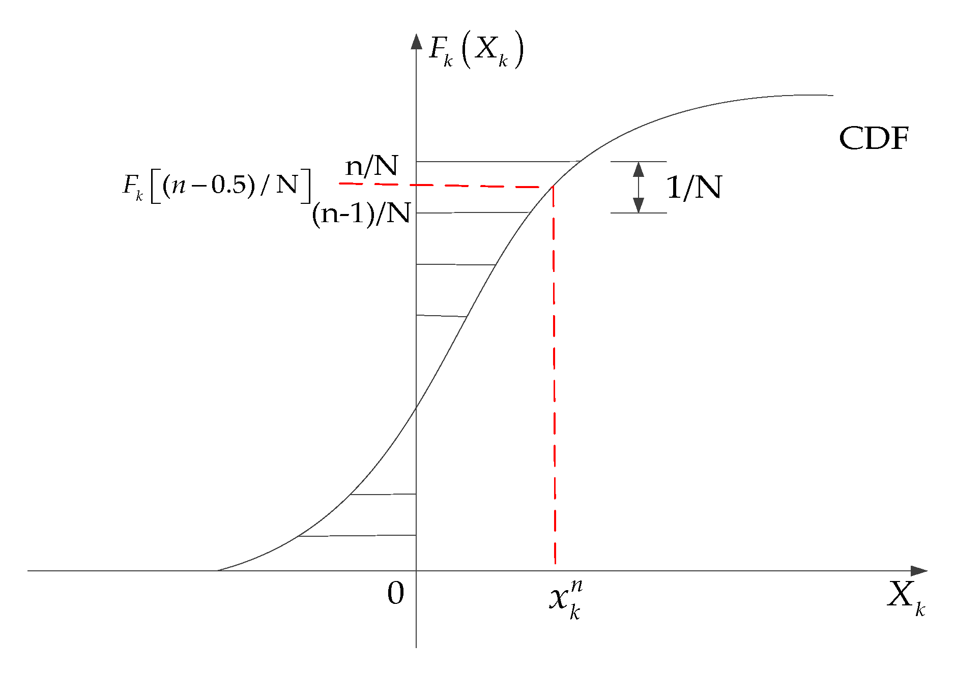
Defining Fk (Xk) as the cumulative distribution function (CDF) of the input variable Xk (k = 1, 2,…, m). Then, the scale of CDF is divided into N equal intervals. A value is extracted in each interval and the sampling value is obtained through the transformation of the inverse function of Fk. The n-th sampling value is as follows:
The sampling procedure is illustrated in Figure 1.
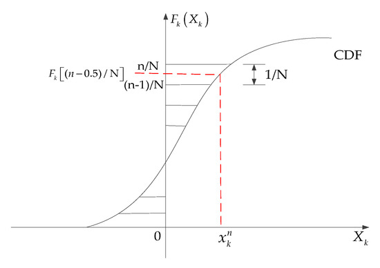
Figure 1.
Sampling procedure of the Latin hypercube sampling (LHS) method.
Since the correlation of derived sampling values does not reflect the practical correlation between input variables, the permutation procedure is required. In the study, the PSO algorithm is used to obtain the desired correlation between sampling values. The detailed procedures are as follows:
Step (1) Generating a population including a number (Np) of particles:
and (k = 1, 2,…, Np) are the position and updating velocity, respectively, of the k-th particle in the j-th iteration. Here, a particle represents a permutation operation.
Step (2) Defining a fitness function F() to represent the quality of . The fitness function is as follows:
where f() is the correlation coefficient between sampling values after performing the permutation operation denoted by on the sampling values; is the desired correlation coefficient. The is better when its fitness function is smaller. Accordingly, let be the best position of the k-th particle among all positions where it has passed, and let be the best position among all (k = 1,2,…,Np).
Step (3) Updating and as follows:
where, are the learning factors; e is the inertial weight; and are random numbers between 0 and 1.
Step (4) Calculating the fitness functions for all particles in the j + 1 iteration. Comparing the current position of the k-th particle with , and set to be the better one of them. Then, set be the best one of all . Then, if the permutation operation denoted by can make f() closer to the desired correlation coefficient, the corresponding permutation operation is made on the sampling values; otherwise, no permutation operation is performed.
Step (5) Iterative process stops when the correlation coefficient between samples reaches a desired value; otherwise, back to step 3 and the iteration number increases by one.
2.1.2. Simultaneous Backward Reduction Technique
In the study, the simultaneous backward reduction technique is used to reduce the number of generated scenarios. A scenario can be defined as follows:
where represents i-th scenario; Ns is the number of generated scenarios; is the s-th element of the i-th scenario; l is the length of the scenario. Accordingly, the Kantorovich distance between scenario i and scenario j is as follows:
According to above definitions, the procedures of using the simultaneous backward reduction technique to reduce the number of generated scenarios are as follows:
Step (1) Deleting the scenario that is closest to all the other scenarios. The scenario satisfies the following equation:
where is the occurrence probability of s-th scenario.
Step (2) The number of scenarios decreases by one and selecting the scenario that is closest to the deleted scenario using the following equation:
Step (3) Changing the occurrence probability of the scenario using the following equation:
Step (4) Back to step 1 if the number of remaining scenarios is larger than the specified number; otherwise, the reduction process stops.
2.2. Verification of the Effectiveness of the Active Power Adjustments of DGs under Extreme Overvoltage Scenarios
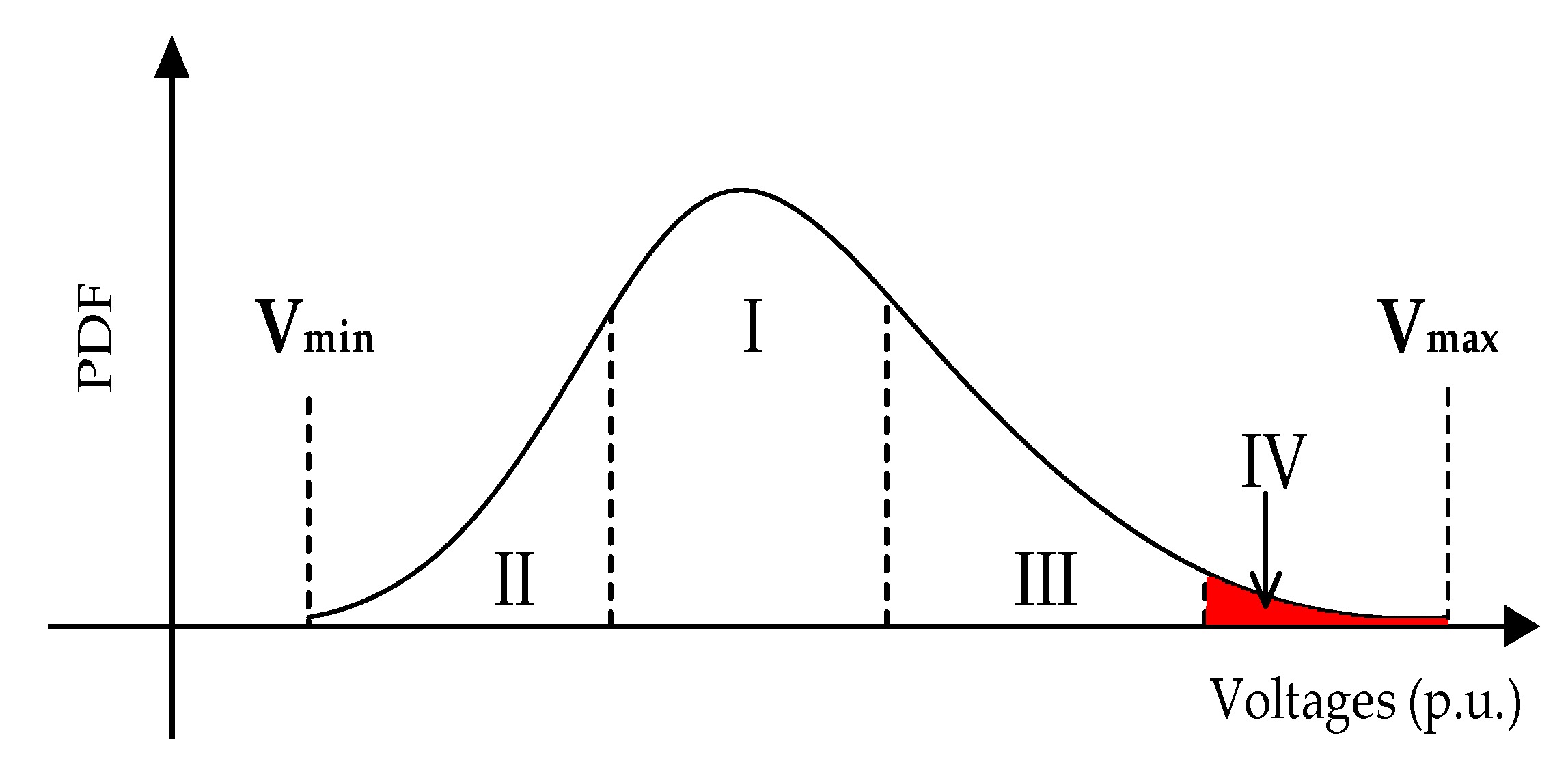
Based on the generated scenarios of active power outputs of DGs and load consumption, the PDF of bus voltages in regional power grids can be obtained and an example of the PDF of bus voltages is shown in Figure 2. It can be seen that the area I represents the qualified voltage area while area IV is the extreme overvoltage area. Area II and III are the low voltage area and overvoltage area, respectively, in which the reactive power adjustments of DGs and VAR compensators can meet the demand of voltage management. In the extreme overvoltage area (area IV), the active power adjustments of DGs can be used to manage voltages. The effectiveness of such a means for voltage management is validated in this section.

Figure 2.
Probability distribution function (PDF) of Bus Voltages in regional power grid.
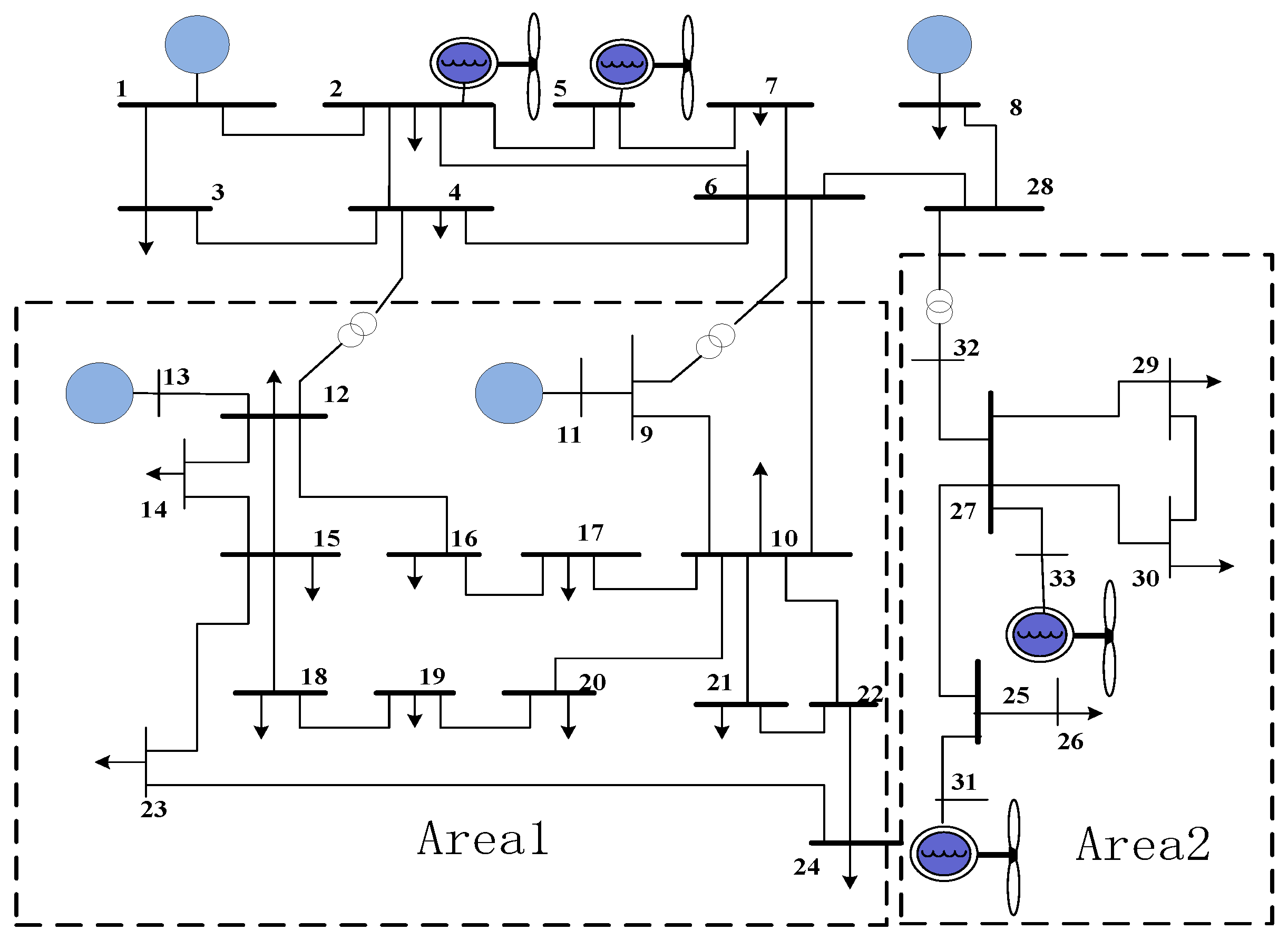
The modified IEEE 30-bus system is selected as the simulation system, as shown in Figure 3, in which four DFIG-based wind turbines (WTs) are connected to bus 2 (WT2), bus 5 (WT5), bus 31 (WT31) and bus 33 (WT33), two small hydropower plants (HPs) are connected to bus 11 (HP11) and bus 13 (HP13). Detailed parameters of the system and DGs are given in the Section 4. It is assumed that the required range of the bus voltage is 0.94 p.u.–1.06 p.u.

Figure 3.
Modified IEEE-30 Bus System.
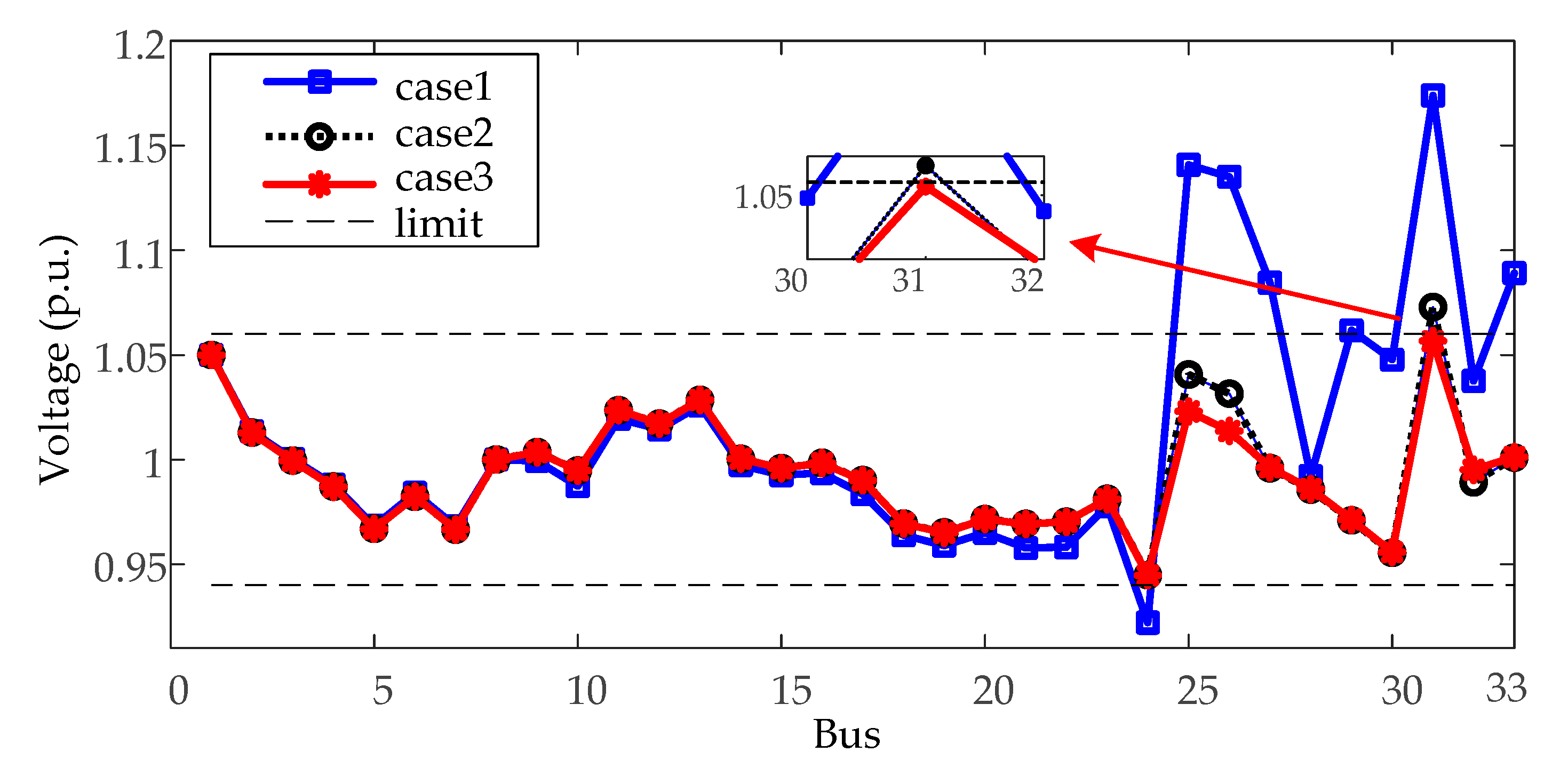
Three cases studies were conducted under the extreme overvoltage scenario. The power outputs of DGs, which are connected in the distribution network, under the extreme overvoltage scenario are listed in Table 1. In case 1, voltage management is not performed; in case 2, the reactive power adjustments of DGs and VAR compensators are used to manage voltages; in case 3, the active and reactive power adjustments of DGs and VAR compensators are used to manage voltages. The power flow results of three cases are listed in Table A1 in Appendix and illustrated in Figure 4. It can be seen that, in case 1, there are extreme overvoltage problems, e.g., bus 25, bus 26 and bus 31, and low voltage problem, e.g., bus 24. In case 2, power outputs of DGs after adjustments are listed in Table 1 and the location and size of VAR compensators are listed in Table A2 in Appendix. It can be seen that, in this case, WT31 absorbs reactive power to alleviate extreme overvoltage at bus 31; however, as shown in Figure 4, an overvoltage problem still occurs at bus 31. In such a case, an additional investment of VAR compensators is required to regulate voltages due to the limited capabilities of reactive power adjustments of DGs. However, in case 3, the active power curtailment of DGs can help alleviate overvoltage. The power outputs of DGs in case 3 are listed in Table 1, it can be seen that the active power output of WT31 is reduced and overvoltage at bus 31 is alleviated. Therefore, it can be concluded that the active power adjustments of DGs can be used to effectively improve the voltage profile under extreme overvoltage scenarios. Therefore, the active power adjustment of DG can be considered in the RPP model to deal with extreme overvoltage scenarios and obtain an optimal allocation of VAR compensators. As a result, the cost of VAR compensator investment can be reduced.

Table 1.
Power outputs of distributed generations (DGs) under the extreme voltage scenario.

Figure 4.
Bus voltages of the regional power grid.
2.3. Proposed RPP Model Based on the Active and Reactive Power Adjustments of DGs
Based on typical scenarios of active power outputs of DGs and loads, a novel RPP model considering the active and reactive power adjustments of DGs is proposed. Since the active power curtailment of DGs will reduce the profits of power generation companies, the objective of the proposed RPP model is to minimize the cost of VAR compensator investment and the lost profits of power generation companies for active power curtailment of DGs. Moreover, to accurately characterize the VAR compensator investment cost, the life cycle cost (LCC) of VAR compensator is used to represent the total cost over its entire life cycle.
Objective 1: Minimize the equivalent annual cost of VAR compensator investment.
where Li is the life cycle cost of the VAR compensator at i-th bus; if a VAR compensator is installed at i-th bus, ki = 1; otherwise, ki = 0; Nb is the number of buses in the system; r is annual discount rate; n is the number of usable years of the VAR compensator; CIi, CMi and CDi are, respectively, the initial investment cost, operating maintenance cost and the scrap cost of the VAR compensator.
Objective 2: Minimize the expected cost of active power curtailment under typical scenarios
where Ns is the number of generated typical scenarios; G is the number of DGs that are used to regulate voltages by adjusting their active power outputs; c3 is the retail tariff; T is the number of annual operating hours; is the expected power output of i-th DG under s-th scenario; is the actual power output of i-th DG under s-th scenario after the active power curtailment.
According to the objective 1 and objective 2, the objective function of the proposed RPP model can be described as follows:
Moreover, a penalty term associated with voltage magnitudes can be added in the objective Equation (12) to ensure bus voltages within the acceptable range as follows:
where the third part of the objective Equation (13) is the penalty term; is the penalty factor; is the voltage of i-th bus under s-th scenario; and are, respectively, the lower and upper limits of bus voltages.
Finally, the proposed RPP model can be described as follows:
where and are, respectively, active and reactive demands at node i under s-th scenario; is the reactive power output of i-th VAR compensators under s-th scenario; is the reactive power output of i-th DG under s-th scenario; is the bus voltage angle difference; and are, respectively, the upper and lower limits of active power output of i-th DG; and are, respectively, the upper and lower limits of reactive power output of i-th DG; and are, respectively, the upper and lower limits of reactive power output of i-th VAR compensators. Equation (16) represents active and reactive power balance constraints under s-th scenario; the Equation (17) represents the limits of active and reactive power adjustments of i-th DG under s-th scenario; the Equation (18) represents the limit of reactive power output of i-th VAR compensator under s-th scenario.
It can be found that the minimum of the sum of the second part and third part in the objective Equation (13) is zero when all bus voltages are within the acceptable range and active power adjustments of DGs are not required. In such a case, the bus voltages can be effectively managed by the installed VAR compensators and reactive power adjustments of DGs. However, when the VAR compensators and reactive power adjustments of DGs cannot meet the requirement of voltage management under extreme overvoltage scenarios, the active power adjustments of DGs are used in the proposed RPP model.
The model Equation (15)–(18) is formulated as a mixed integer nonlinear programming (MINLP) problem, the discrete variables are the location (k1, k2,…, ki), size (, ) and reactive power output () of VAR compensator that discretely provides reactive power. Continuous variables are the active and reactive power outputs of DGs, voltage magnitudes, voltage angles and reactive power output of the VAR compensator that can output reactive power continuously.
3. Proposed Primal-Dual Interior Point Based Particle Swarm Optimization Algorithm
Since the proposed RPP model is formulated as a MINLP problem, a PDIP-based PSO algorithm is developed to effectively solve the proposed model.
3.1. Primal-Dual Interior Point Method
The brief descriptions about PDIP are given in this subsection. An optimization problem can be formulated in the following compact form:
where X is the vector of decision variables; f(X) is the objective function; H(X) represents equality constraints; G(X) represents inequality constraints. The inequality constraints can be transformed into equality constraints by adding slack variable Z and a logarithmic barrier function can be added in the objective function to penalize the slack variable. The corresponding model is as follows:
where γ is the penalty coefficient. Based on Equation (20), the augmented Lagrangian function can be formulated as follows:
where λ and μ are Lagrangian multipliers of equality constraints. Corresponding first order Karush-Kuhn-Tucker (KKT) optimality conditions are as follows:
where .
Then, applying the newton method to the KKT condition Equation (22), the following newton equations can be derived:
where . In each iteration of the newton method, the variables can be updated using the following equations:
where is the step size. In addition, in each iteration, the coefficient γ can be update using the following equation:
where σ is the centering parameter between 0 and 1; n is the number of slack variables. Repeating Equations (23)–(25) until the convergence conditions are satisfied.
3.2. Proposed PDIP Based PSO Algorithm
The proposed PDIP-based PSO algorithm has similar procedures as step 1-step 5 in Section 2.1.1 with the following differences.
Step (1) Generating a population including a number (Np) of particles: and (k = 1, 2,…, Np). Here, a particle represents the location (ki) and size (, ) of a VAR compensator.
Step (2) Defining a fitness function F(), namely objective Equation (15), to represent the quality of . For a given particle (), the fitness function can be obtained by solving the model (15)–(18) with fixed variables (ki, , ) using the PDIP method. Moreover, it should be mentioned that the discrete variables () are firstly assumed to be continuous and the PDIP method is used to search the optimal solution. After obtaining the optimal solution, the derived continuous variables () are rounded and fixed. Then, the optimization model is solved again. The larger the fitness function, the better is the .
Step (3) Updating and using (3).
Step (4) Calculating the fitness functions for all particles in the j + 1 iteration and resetting and .
Step (5) Iterative process stops when the number of iterations reaches a preset maximum or other termination conditions are satisfied, and output as the result; otherwise, go to step (3) and the iteration number increases by one.
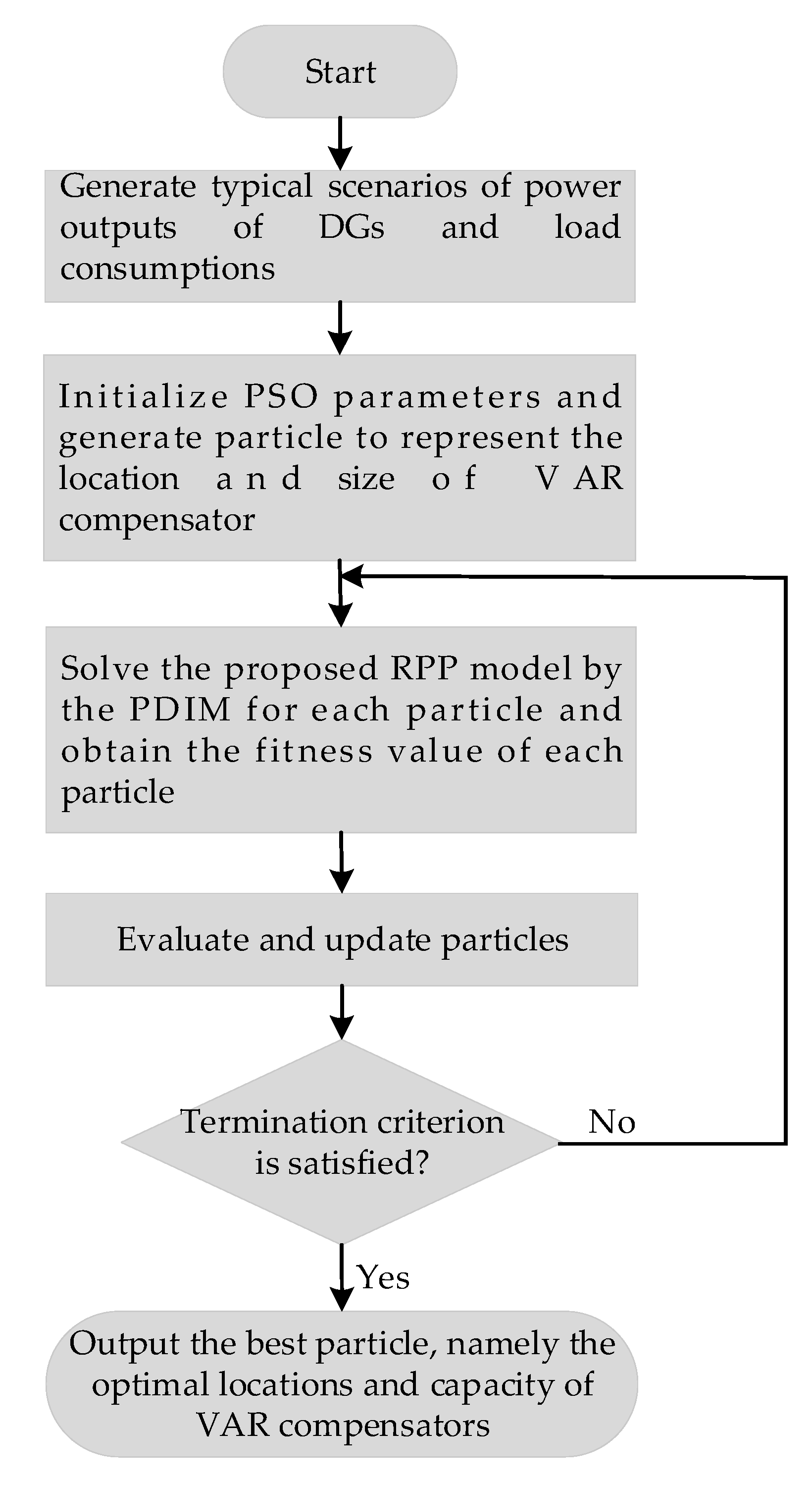
The flow chart of the proposed algorithm is illustrated in Figure 5.
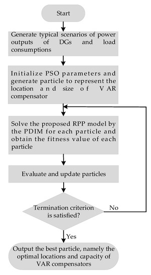
Figure 5.
The flow chart of proposed algorithm.
4. Case Studies
4.1. System Data and Simulation Parameters
The effectiveness of the proposed RPP model is verified on the modified IEEE 30-bus system shown in Figure 3. The WT2 and WT5 have a rated capacity of 50 MVA and the rest of WTs have a rated capacity of 20 MVA. The HP11 and HP13 have a rated capacity of 20 MVA. The correlation coefficients between the power outputs of WT2 and WT5, WT31 and WT33 are both 0.4, and the correlation coefficient between HP11 and HP13 is 0.5. The initial investment parameter CI for shunt capacitors and shunt reactors is 70 RMB (12 USD)/kVAR, for SVG is 300 (50 USD) RMB/kVAR. The annual operating maintenance cost parameter CM is 6% of the initial investment, and the scrap cost parameter CD is 2% of the initial investment. The discount rate r is 0.1 and the usable duration n is 10 years. The penalty factor cp is 1 × 10¹⁰. The retail tariff of wind power c3 is 0.3 RMB (0.05 USD)/kWh. The number of typical scenarios of power outputs of DGs (WTs, HPs) and load consumptions is 50. In the proposed PDIP-based PSO algorithm, the number of particles is 100, the number of iterations is 400, the weight factor e is 0.5, and the learning factors c1 and c2 are both 2. The simulations were conducted with a desktop with a 2.5-GHz Intel Core i5-3210 CPU (Intel, Santa Clara, CA, USA) and 4.00 GB of RAM (DDR3, Samsung, Seoul, South Korea).
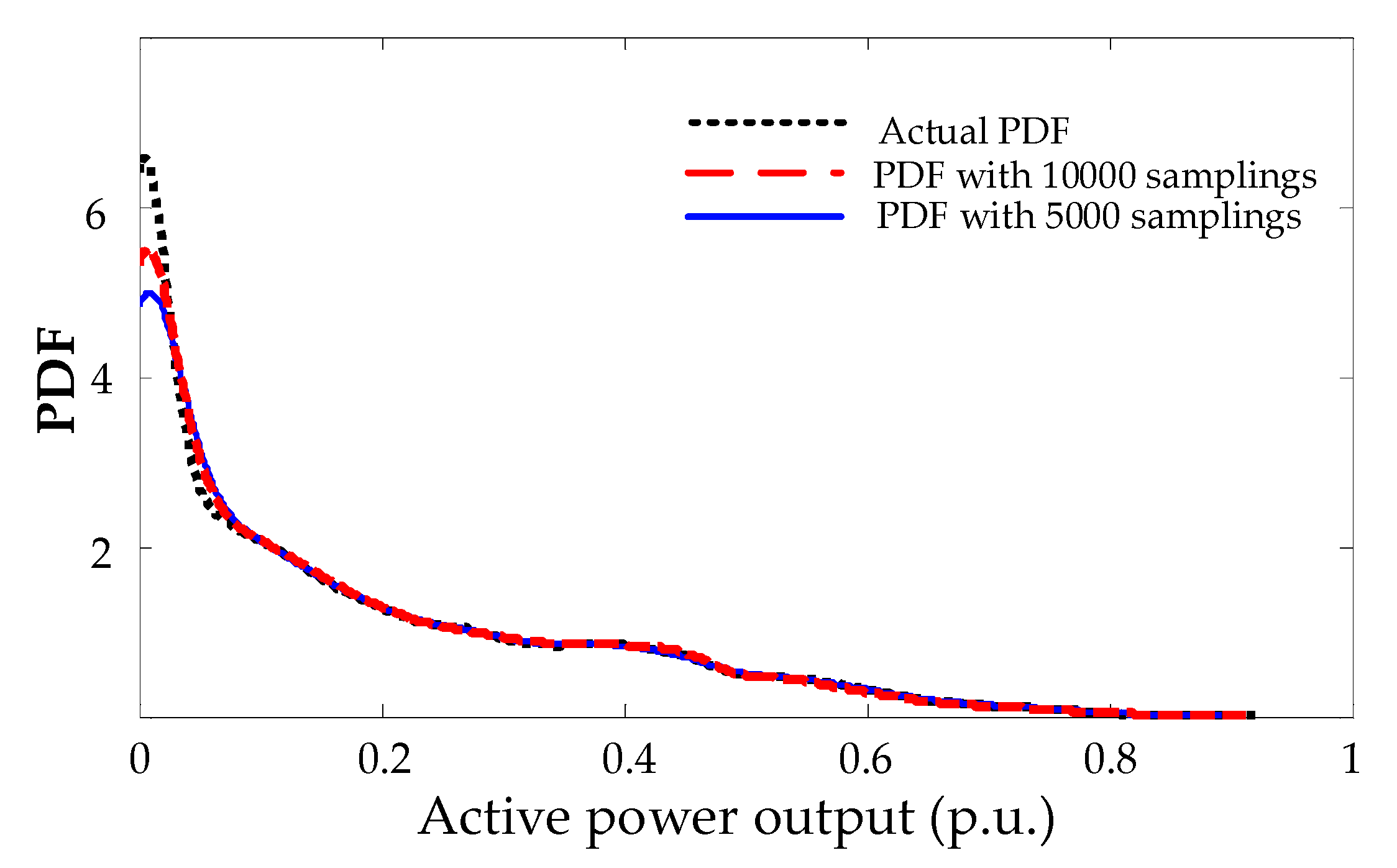
In the study, LHS method is used to obtain 5000 sampling values for each WT and HP from their historical statistic CDFs and for loads from typical load curves. Take the WT2 as an example, the effectiveness of the LHS method is validated in Figure 6. It can be seen that the PDF of sampling values of active power output of WT2 is very closer to its actual PDF. In particular, with the increasing number of samplings, the fitting effect is better. After obtaining sampling values of all the WTs and HPs, the PSO algorithm is used to derive the desired correlation coefficients by performing the permutation process. After that, the number of generated scenarios is reduced to be 50 by using the simultaneous backward reduction technique.
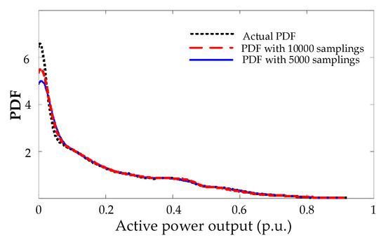
Figure 6.
PDF of sampling values.
4.2. Case Studies Results
After obtaining 50 typical scenarios, four RPP models were implemented and compared in this section. Case 1 is the RPP model proposed in this paper, in which VAR compensators, the active and reactive power adjustments of DGs are coordinated to regulate voltages under extreme overvoltage scenarios. In case 2, VAR compensators and reactive power adjustments of DGs are combined to regulate voltages under extreme overvoltage scenarios. In case 3, the active and reactive power adjustments of DGs are used to regulate voltages under extreme overvoltage scenarios. In case 4, only VAR compensators are used to regulate voltages.
To reduce the search space of the proposed algorithm, the over-limit probability analysis of bus voltages is performed to determine the candidate installation buses of VAR compensators. Power flow study is carried out for each scenario (5000 scenarios in total) and the over-limit probability of each bus is calculated according to the following equation:
where are and , respectively, the over-upper limit probability and over-lower limit probability of i-th bus; Nt is the number of total scenarios; is the number of scenarios in which overvoltage occurs at i-th bus; is the number of scenarios in which low voltage occurs at i-th bus. According to statistic results listed in Table 2, the nodes 18, 19, 20, 21, 22, 24 are candidate installation buses of shunt capacitors because they have high over-lower limit probabilities. The buses 25, 26, 27, 29, 32, 33 are candidate installation buses of shunt reactors because they have high over-upper limit probabilities. The bus 30 and bus 31 are candidate installation buses of SVGs because both the over-lower limit probability and the over-upper limit probability are high.
Table 2.
Probability of over-limit of bus voltage.
The reactive power planning results of the four RPP models are listed in Table 3. In case 4, voltages are regulated by VAR compensators only; therefore, the required installation capacity of VAR compensators is the largest. In case 2, VAR compensators and reactive power adjustments of DGs are combined to regulate voltages under extreme overvoltage scenarios such that the installation capacity of VAR compensators can be reduced. In case 1, VAR compensators, active and reactive adjustment of DGs are coordinated to regulate voltages under the extreme overvoltage scenarios; therefore, the installation capacity of VAR compensators can be further reduced. In case 3, since extreme overvoltage are only regulated by active and reactive power adjustments of the DGs, the installation capacity of VAR compensators is the lowest.
Table 3.
Results of four reactive power planning (RPP) Models.
In addition, the serial number of the scenario that requires active power adjustments of DGs under four cases are listed in Table 4. Accordingly, the required active power curtailment value under each scenario is also listed in Table 4. It can be seen the number of scenarios requiring active power curtailment in case 3 is larger than the one in case 1, because VAR compensators can help alleviate overvoltage in case 1. There is no scenario requiring active power curtailment in case 2 and case 4, because active power adjustment of DG does not participate in regulating overvoltage in the extreme overvoltage scenarios.
Table 4.
Active power curtailment value of DGs under the extreme overvoltage scenario.
The total costs (VAR compensator investment cost plus active power curtailment cost) of four cases are listed in Table 5. It can be seen that case 3 has the minimum VAR compensator investment cost while there are many scenarios that need active power curtailment of DGs (as shown in Table 4). Therefore, it requires large active power curtailment cost, resulting in the largest total cost. Although case 1 requires active power curtailment in a few scenarios when comparing with case 2, the curtailment values are small, and the VAR compensator investment cost can be significantly reduced. Therefore, case 1 has the minimum total cost, which demonstrates the cost-efficiency of the proposed RPP model.
Table 5.
Total costs of four cases.
In addition, considering case 2 as a benchmark case, the percentage of the VAR compensator investment saving at power grid side and the percentage of lost profits of power generation companies are listed in Table 5. For the proposed RPP model in case 1, the generation companies lose 0.43% of profits while the percentage of the VAR compensator investment saving reaches 29.9%. Therefore, the power grid can offer appropriate compensation to power generation companies so that generation companies can accept the proposed RPP model. In case 3, although the power gird side can save 59.7% of the VAR compensator investment cost, generation companies lose 9.6% of profits. In such a case, the lost profit is high and case 3 is unacceptable to power generation companies. Based on above analyses, the proposed RPP model can minimize to the maximum extent the VAR compensator investment cost without requiring large lost profits of power generation companies.
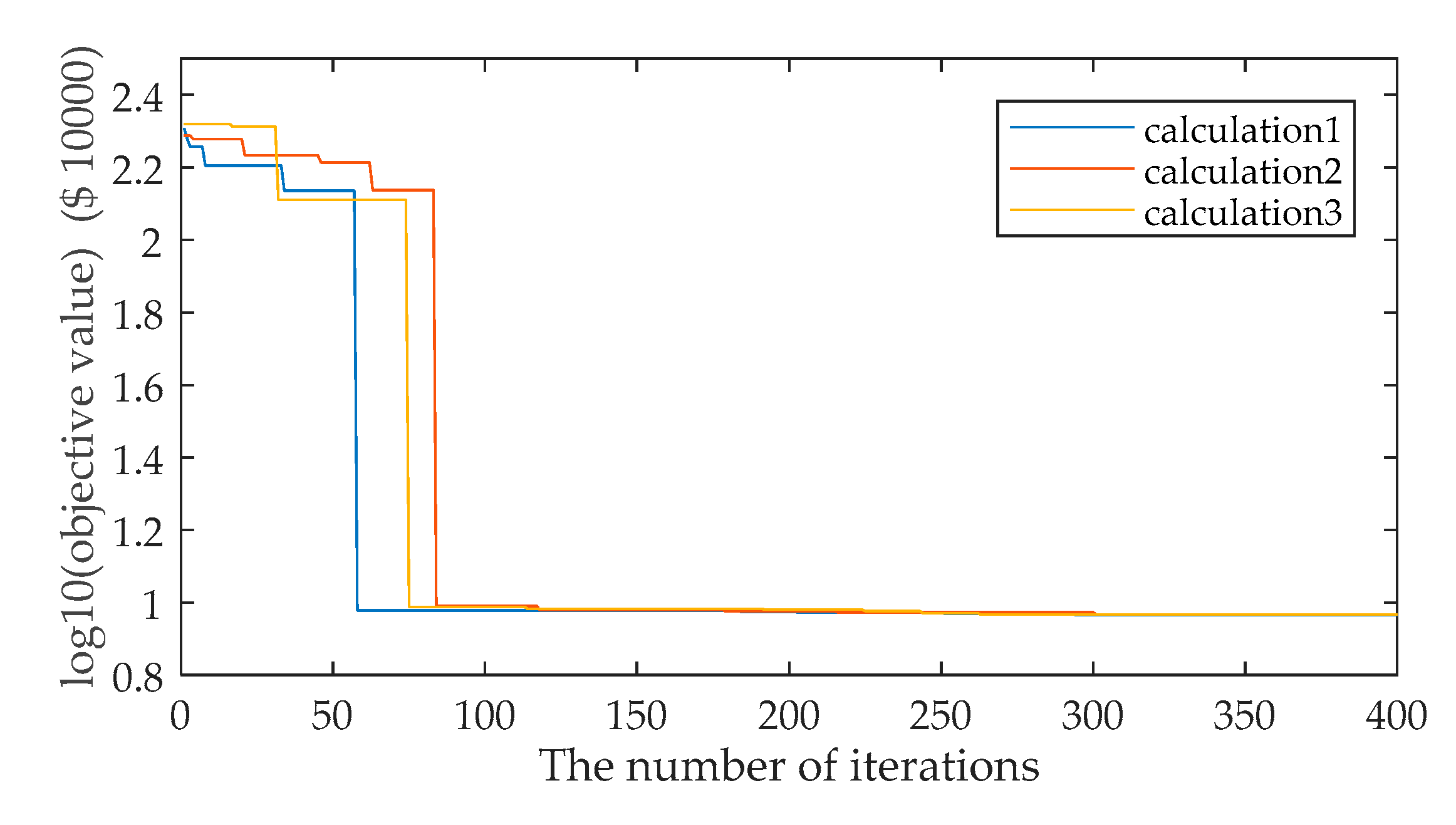
In addition, the iteration process of the proposed algorithm is illustrated in Figure 7. It can be seen that after 350 iterations, an optimal solution of the proposed RPP model can be obtained. It takes almost 90 min to reach the convergence.
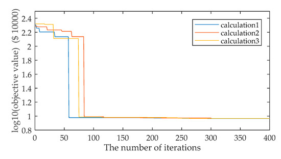
Figure 7.
Iteration process of the proposed algorithm.
5. Discussion
The comparison results of the four types of RPP models are summarized in this section.
From the perspective of the VAR compensators investment cost, case 3 has the minimum VAR compensator investment cost because overvoltage is regulated by the active power and reactive power adjustments of DGs under extreme overvoltage scenarios. Case 4 has the maximum investment cost because only VAR compensators are used to regulate overvoltage under extreme overvoltage scenarios. Compared with case 4, the VAR compensator investment cost can be reduced in case 3 because reactive power adjustment of DG can be used to help alleviate overvoltage under extreme overvoltage scenarios. In case 1, the VAR compensator investment cost can be further reduced because active power adjustment of DG can be used as the additional means to alleviate overvoltage under extreme overvoltage scenarios.
From the perspective of the active power curtailment cost of DG, there is no active power curtailment cost in case 2 and case 4 because the active power adjustment of DG is not used to regulate overvoltage under extreme overvoltage scenarios in these two cases. In case 3, the active power curtailment cost is the largest because only the active and reactive power adjustments of DGs are used to alleviate overvoltage under the extreme overvoltage scenario. However, in case 1, the VAR compensators can also be used to help alleviate overvoltage; therefore, the active power curtailment cost can be reduced.
From the perspective of the total cost, the proposed RPP model in case 1 has the minimum total cost. For case 3, although case 3 has the minimum VAR compensator investment cost, it has the largest active power curtailment cost, resulting in the largest total cost. For case 2 and case 4, although there is no active power curtailment cost, they have higher VAR compensator investment cost than case 1. Consequently, they have higher total costs than case 1.
Above analyses demonstrate the economic efficiency of the proposed RPP model. In addition, the feasibility of the proposed RPP model is also analyzed. As shown in Table 5, for the proposed RPP model in case 1, the generation companies lose 0.43% of profits while the percentage of VAR compensator investment saving at power gird side reaches 29.9%. Therefore, the power grid can offer appropriate compensation to power generation companies so that generation companies can accept the proposed RPP model.
6. Conclusions
To economically deal with extreme overvoltage problems, this paper proposes a novel RPP model based on the active and reactive power adjustments of DGs. Firstly, several typical scenarios of power outputs of DGs and load consumption are produced. Secondly, based on typical scenarios, an RPP model considering the active and reactive power adjustments of DGs is proposed to determine the optimal allocation of VAR compensators. Finally, the proposed RPP model is solved by the proposed PDIP-based PSO algorithm. The simulation results demonstrate that the proposed model can not only significantly reduce the VAR compensator investment, but also reduce the total cost of voltage management in power systems.
Author Contributions
Conceptualization, Y.S., F.S. and D.K.; Methodology, Y.S. and F.S.; Software, Y.S. and F.S.; Validation, Y.S. and F.S.; Formal Analysis, L.L. and B.Z.; Investigation, Y.C. and B.Z.; Resources, L.L. and B.Z.; Data Curation, L.L. and Y.C.; Writing-Original Draft Preparation, F.S. and Y.S.; Writing-Review & Editing, Y.C. and D.K.; Visualization, Y.C.; Supervision, D.K.; Project Administration, Y.S.; Funding Acquisition, Y.S.
Funding
This research received no external funding.
Conflicts of Interest
The authors declare no conflict of interest.
Appendix
Table A1.
Power flow results of three cases.
Table A1.
Power flow results of three cases.
| Bus | Case 1 | Case 2 | Case 3 | |||
|---|---|---|---|---|---|---|
| Cases | Voltage Mag. (p.u.) | Voltage Angle (deg.) | Voltage Mag. (p.u.) | Voltage Angle (deg.) | Voltage Mag. (p.u.) | Voltage Angle (deg.) |
| 1 | 1.050 | 0.000 | 1.050 | 0.000 | 1.050 | 0.000 |
| 2 | 1.014 | −2.493 | 1.013 | −2.485 | 1.013 | −2.582 |
| 3 | 1.000 | −3.772 | 0.999 | −3.761 | 0.999 | −3.916 |
| 4 | 0.988 | −4.597 | 0.987 | −4.584 | 0.987 | −4.777 |
| 5 | 0.968 | −6.399 | 0.967 | −6.393 | 0.967 | −6.566 |
| 6 | 0.984 | −5.101 | 0.982 | −5.081 | 0.982 | −5.336 |
| 7 | 0.968 | −6.273 | 0.967 | −6.261 | 0.967 | −6.482 |
| 8 | 1.000 | −3.720 | 1.000 | −3.739 | 1.000 | −4.159 |
| 9 | 0.999 | −8.174 | 1.004 | −8.159 | 1.004 | −8.404 |
| 10 | 0.987 | −10.872 | 0.995 | −10.833 | 0.995 | −11.073 |
| 11 | 1.019 | −6.264 | 1.024 | −6.266 | 1.024 | −6.510 |
| 12 | 1.014 | −9.581 | 1.017 | −9.510 | 1.017 | −9.722 |
| 13 | 1.026 | −8.533 | 1.029 | −8.467 | 1.028 | −8.679 |
| 14 | 0.997 | −10.621 | 1.000 | −10.543 | 1.000 | −10.757 |
| 15 | 0.993 | −10.696 | 0.996 | −10.623 | 0.996 | −10.838 |
| 16 | 0.994 | −10.421 | 0.998 | −10.371 | 0.998 | −10.595 |
| 17 | 0.984 | −11.008 | 0.990 | −10.959 | 0.990 | −11.194 |
| 18 | 0.964 | −12.142 | 0.970 | −12.072 | 0.969 | −12.300 |
| 19 | 0.959 | −12.358 | 0.965 | −12.291 | 0.965 | −12.523 |
| 20 | 0.965 | −12.059 | 0.972 | −11.998 | 0.972 | −12.232 |
| 21 | 0.958 | −12.120 | 0.969 | −12.153 | 0.969 | −12.393 |
| 22 | 0.958 | −12.125 | 0.970 | −12.176 | 0.970 | −12.416 |
| 23 | 0.978 | −11.336 | 0.981 | −11.259 | 0.981 | −11.474 |
| 24 | 0.922 | −13.623 | 0.945 | −13.992 | 0.945 | −14.233 |
| 25 | 1.141 | 1.618 | 1.041 | 5.342 | 1.023 | 2.056 |
| 26 | 1.135 | 1.558 | 1.031 | 5.431 | 1.014 | 2.148 |
| 27 | 1.084 | 1.644 | 0.996 | 3.528 | 0.996 | 0.903 |
| 28 | 0.992 | −4.407 | 0.986 | −4.312 | 0.986 | −4.737 |
| 29 | 1.062 | 0.471 | 0.971 | 2.131 | 0.971 | −0.493 |
| 30 | 1.048 | −0.354 | 0.955 | 1.142 | 0.956 | −1.481 |
| 31 | 1.174 | 4.412 | 1.073 | 8.694 | 1.057 | 4.457 |
| 32 | 1.038 | −1.142 | 0.989 | −0.903 | 0.995 | −2.325 |
| 33 | 1.089 | 2.922 | 1.000 | 5.042 | 1.001 | 2.41 |
Table A2.
Location and size of VAR compensator in Case 2.
Table A2.
Location and size of VAR compensator in Case 2.
| Shunt Capacitor | Shunt Reactor | ||||
|---|---|---|---|---|---|
| Bus | 24 | 25 | 26 | 27 | 31 |
| Size (MVAR) | 2 | 3 | 2 | 1 | 2 |
References
- Shen, Y.; Ke, D.; Sun, Y.; Kirschen, D.; Qiao, W. Advanced Auxiliary Control of an Energy Storage Device for Transient Voltage Support of a Doubly Fed Induction Generator. IEEE Trans. Sustain. Energy 2016, 7, 63–76. [Google Scholar] [CrossRef]
- Liserre, M.; Sauter, T.; Hung, J. Future energy systems, integrating renewable energy sources into the smart power grid through industrial electronics. IEEE Ind. Electron. Mag. 2010, 4, 18–37. [Google Scholar] [CrossRef]
- Shen, Y.; Liang, L.; Cui, M.; Shen, F.; Zhang, B. Advanced Control of DFIG to Enhance the Transient Voltage Support Capability. J. Energy Eng. 2018, 144, i2. [Google Scholar] [CrossRef]
- Shen, Y.; Ke, D.; Qiao, W.; Sun, Y.; Kirschen, D.; Wei, C. Transient reconfiguration and coordinated control for power converters to enhance the LVRT of a DFIG wind turbine with an energy storage device. IEEE Trans. Energy Convers. 2015, 30, 1679–1690. [Google Scholar] [CrossRef]
- Seritan, G.; Triştiu, I.; Ceaki, O.; Boboc, T. Power quality assessment for microgrid scenarios. In Proceedings of the 2016 International Conference and Exposition on Electrical and Power Engineering (EPE), Isai, Romania, 20–22 October 2016; pp. 723–727. [Google Scholar]
- Ceaki, O.; Seritan, G.; Vatu, R.; Mancasi, M. Analysis of power quality improvement in smart grids. In Proceedings of the 2017 10th International Symposium on Advanced Topics in Electrical Engineering (ATEE), Bucharest Romania, 23–25 March 2017; pp. 797–801. [Google Scholar]
- Kacejko, P.; Adamek, S.; Wydra, M. Optimal voltage control in distribution networks with dispersed generation. In Proceedings of the Innovative Smart Grid Technologies Conference Europe, Gothenberg, Sweden, 11–13 October 2010. [Google Scholar]
- Vita, V.; Alimardan, T.; Ekonomou, L. The impact of distributed generation in the distribution networks’ voltage profile and energy losses. In Proceedings of the 9th IEEE European Modeling Symposium on Mathematical Modelling and Computer Simulation, Madrid, Spain, 6–8 October 2015; pp. 260–265. [Google Scholar]
- Vita, V. Development of a decision-making algorithm for the optimum size and placement of distributed generation units in distribution networks. Energies 2017, 10, 1433. [Google Scholar] [CrossRef]
- Nieto, A.; Vita, V.; Maris, T.I. Power quality improvement in power grids with the integration of energy storage systems. Inter. J. Eng. Res. Technol. 2016, 5, 438–443. [Google Scholar]
- Sharma, N.; Ghosh, A.; Varma, R. A novel placement strategy for FACTS controllers. IEEE Trans. Power Deliv. 2003, 18, 982–987. [Google Scholar] [CrossRef]
- MÍnguez, R.; Milano, F.; Conejo, A. Optimal Network Placement of SVC Devices. IEEE Trans. Power Syst. 2007, 22, 1851–1860. [Google Scholar] [CrossRef]
- Nguyen, K.; Fujita, G.; Dieu, V. Optimal placement and sizing of Static Var Compensator using Cuckoo search algorithm. In Proceedings of the IEEE Congress on Evolutionary Computation (CEC), Sendai, Japan, 25–28 May 2015; pp. 267–274. [Google Scholar]
- Liu, X.; Liu, T.; Li, X. Optimal reactive power planning in distribution system with wind power generators. Power Syst. Prot. Control 2010, 38, 130–135. [Google Scholar]
- Liu, P.; Gu, L. Optimization of reactive power planning for power system containing wind farms. Power Syst. Technol. 2010, 7, 175–180. [Google Scholar]
- Wang, M.; Qiu, C. Chance-constrained reactive power planning of wind farm integrated distribution system considering voltage stability. In Proceedings of the 12th IEEE International Conference on Electronic Measurement and Instruments (ICEMI), Qingdao, China, 16–18 July 2015; pp. 30–35. [Google Scholar]
- Dadkhah, M.; Venkatesh, B. Cumulant based stochastic reactive power planning method for distribution systems with wind generators. IEEE Trans. Power Syst. 2012, 27, 2351–2359. [Google Scholar] [CrossRef]
- Yang, S.; Luo, N.; Han, N. Study on dynamic reactive power optimization dispatching for a local power system. Power Syst. Prot. Control 2013, 47, 122–126. [Google Scholar]
- Dukpa, A.; Venkatesh, B.; Chang, L. Fuzzy stochastic programming method: Capacitor planning in distribution systems with wind generators. IEEE Trans. Power Syst. 2011, 26, 1971–1979. [Google Scholar] [CrossRef]
- Fang, X.; Li, F.; Wei, Y.; Azim, R.; Xu, Y. Reactive power planning under high penetration of wind energy using Benders decomposition. IET Gener. Transm. Distrib. 2015, 9, 1835–1844. [Google Scholar] [CrossRef]
- Xu, Q.; Yang, Y.; Liu, Y.; Wang, X. An Improved Latin Hypercube Sampling Method to Enhance Numerical Stability Considering the Correlation of Input Variables. IEEE Access 2017, 5, 15197–15205. [Google Scholar] [CrossRef]
- Dupacova, J.; Growe, N.; Romisch, W. Scenario reduction in stochastic programming: An approach using probability metrics. Math. Program. 2003, 95, 493–511. [Google Scholar] [CrossRef]
- Chen, Q.; Zhao, X.; Gan, D. Active-reactive scheduling of active distribution system considering interactive load and battery storage. Prot. Control Mod. Power Syst. 2017, 2, 320–330. [Google Scholar] [CrossRef]
- Shen, Y.; Cui, M.; Wang, Q.; Shenm, F.; Zhang, B. Comprehensive Reactive Power Support of DFIG Adapted to Different Depth of Voltage Sags. Energies 2017, 10, 808. [Google Scholar] [CrossRef]
- Wang, L.; Gao, H.; Zou, G. Modeling methodology and fault simulation of distribution networks integrated with inverter-based DG. Prot. Control Mod. Power Syst. 2017, 2, 370–378. [Google Scholar] [CrossRef]
© 2018 by the authors. Licensee MDPI, Basel, Switzerland. This article is an open access article distributed under the terms and conditions of the Creative Commons Attribution (CC BY) license (http://creativecommons.org/licenses/by/4.0/).