Abstract
The grounding grid is a key part of substation protection, which provides safety to personnel and equipment under normal as well as fault conditions. Currently, the topology of a grounding grid is determined by assuming that its orientation is parallel to the plane of earth. However, in practical scenarios, the assumed orientation may not coincide with the actual orientation of the grounding grid. Hence, currently employed methods for topology detection fails to produce the desired results. Therefore, accurate detection of grounding grid orientation is mandatory for measuring its topology accurately. In this paper, we propose a derivative method for orientation detection of grounding grid in high voltage substations. The proposed method is applicable to both equally and unequally spaced grounding grids. Furthermore, our method can also determine the orientation of grounding grid in the challenging case when a diagonal branch is present in the mesh. The proposed method is based on the fact that the distribution of magnetic flux density is perpendicular to the surface of the earth when a current is injected into the grid through a vertical conductor. Taking the third order derivative of the magnetic flux density, the main peak coinciding with the position of underground conductor is accurately obtained. Thus, the main peak describes the orientation of buried conductor of grounding grid. Simulations are performed using Comsol Multiphysics 5.0 to demonstrate the accuracy of the proposed method. Our results demonstrate that the proposed method calculate the orientation of grounding grid with high accuracy. We also investigate the effect of varying critical parameters of our method.
1. Introduction
The grounding grid provides a low impedance path from electrical equipment to earth, ensuring protection from high lightening and short circuit current under fault conditions [1,2]. The grounding grid also maintains step and touch voltages within limit, ensuring the safety of personnel inside the premises under normal and fault conditions. A typical grounding grid comprises of bare conductors buried 0.3 m to 0.5 m (12 in to 18 in) below the earth’s surface and spaced equally or unequally from 3 m to 7 m (10 ft to 20 ft) apart. These bare conductors are placed in grid or mesh pattern and are securely bonded together at cross connections. Vertical conductors are installed at major equipment points and structures such as lightning arresters and power transformers etc. These vertical conductors are the only access points to the grounding grid. The buried mesh of bare conductors is spread over the entire area of the switch-yard and often a few meters beyond the fence [3]. Vertical grounding conductors are also connected to grounding grid, penetrating deeper into the lower resistivity soil. These vertical grounding conductors effectively dissipate fault currents into the earth, whenever a two layer or multilayer soil is encountered [3].
The buried bare conductors are subjected to corrosion under decomposing nature of earth. This phenomena effects conductivity of the grounding grid and with the passage of time, it may result in a broken grid [4]. Inefficient or broken grounding grid represents a critical fault and hidden danger to equipment, life and smooth operation of power grid.
Electromagnetic field methods [5,6,7], electric circuit analysis [4,8,9], electrochemical methods [10,11] and optimization techniques [12,13] have been extensively used for corrosion and breakpoint diagnosis. However, in the case of unknown grounding grids topology and orientation are those two distinctive parameters that must be evaluated before applying any fault diagnosis technique. The topology of a grounding grid is defined as the formation taken by the interconnections of grounding grid conductors whereas orientation is the location of grounding grid with reference to the plane of earth.
Configuration drawings providing topology and orientation references are often lost and mishandled. Excavation is not used to determine grounding grid topology and orientation because it not only requires power outage but has also proved itself as poor time and cost effective solution.
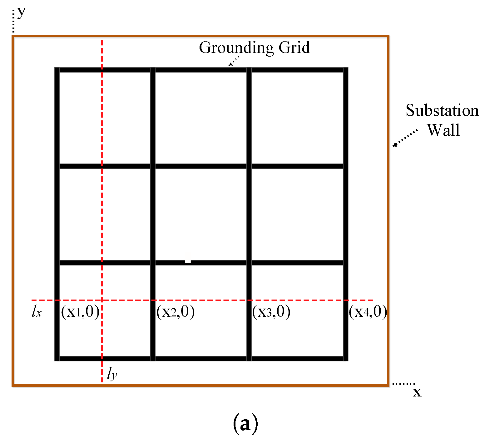
A method for topology detection is developed in [14] based on the concept of regret. This method cannot detect the complete topology of grounding grid when a broken branch is encountered. Moreover, this method requires orientation of grounding grid before it can be applied for topology detection. Reference [15] measures the grounding grid configuration by employing transient electromagnetic method (TEM). Secondary magnetic fields due to induced eddy currents in the grounding grid are recorded. Grounding conductors lie under points of minimum magnetic field intensity. The flaw in [15] is that the orientation of grounding grid is presumed to be parallel to the plane of the earth which in real scenarios is unknown. In [16], line derivative is used to configure the topology of grounding grid. The location of peaks obtained by taking the derivative of magnetic flux density represents the position of ground branches. It can be seen in Figure 1a, where the grounding grid is located parallel to the substation boundary such that the location of each ground branch is a function of either x or y. Therefore, line derivative and is used to determine the location of ground branches lying along x-axis and y-axis, respectively. Although [16] works well with the assumption that grounding grid is located parallel to the plane of the earth (substation boundary) but a major flaw arises in circumstances where grounding grid is not lying parallel to the plane of the earth as shown in Figure 1b. Here, location and thus the magnetic flux density of ground branches is described as a function of both x and y. Hence, [16] will not be able to detect grounding grid topology using line derivative approach as shown in Figure 1b. Furthermore, in light of the above discussion, [16] will also fail by taking the diagonal branch into account.

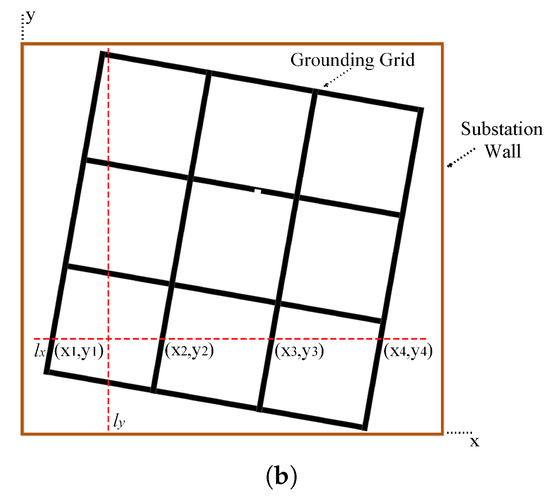
Figure 1.
Depending on substation design requirements, grounding grid can be located at any angle with reference to substation boundary. (a) Orientation of grounding grid is assumed parallel to the substation boundary. For instance, the location of ground branches below are a function of x and similarly the location of ground branches below are a function of y. Therefore, line derivative technique can be used to determine grounding grid topology. (b) Grounding grid is located at an angle with the substation boundary. Here, location of branches with respect to xy-plan are a function of both x and y. On the other hand, is only a function of x and similarly is a function of y thus line derivatives and will produce incorrect results.
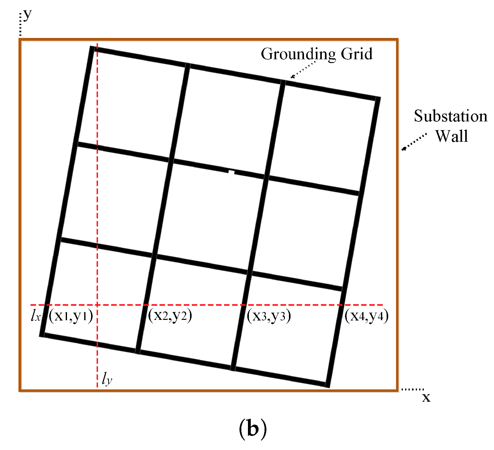
The orientation of grounding grid has first determined by [17] using circular derivative and then applied line and circle derivative to measure the complete topology. In order to generate satisfactory results from the approach used in [17], grounding grid must be equally spaced as shown in Figure 2a. In contrast, the topology of grounding grid is based on substation equipment layout and therefore it may not necessarily be equally spaced grid as depicted in Figure 2b. Topology of grounding grid may vary with time, depending on the changes in grid station layout. Modifications in grounding grid includes additional vertical conductors, varying space between adjacent branches and varying lengths or orientation of ground branches [15].
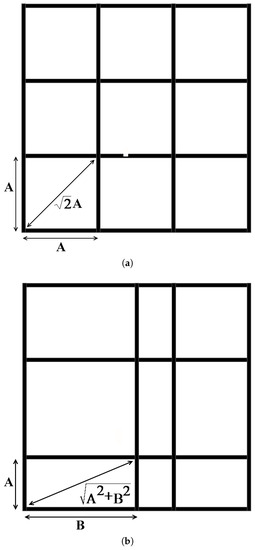
Figure 2.
Based on substation equipment layout, grounding grid can be configured as equally spaced or unequally spaced. (a) Equally spaced grounding grid configuration have all the branches of equal length. (b) Unequally spaced grounding grid have branches of unequal lengths.
The method by [17] does not take into account the challenging case of a diagonal branch present in an unequally spaced grid. The presence of a diagonal branch in an equally spaced square grid will reduce the angular displacement between ground branches from 90 to 45. Thus, the spacing between ground branch distinguishing peaks will also reduce. In conditions where a diagonal branch is connected to vertical conductor and side to side ratio of grounding grid is changed from 1:1. The angular displacement between a normal and a diagonal branch reduces below 45 and becomes so small that the derivative peaks will overlap with each other. These overlappings will produce fake peaks and as a consequence, [17] will not be able to distinguish between real and fake peaks describing the orientation of ground branches.
Contributions: In this paper, we propose the electromagnetic and derivative method to measure the orientation of grounding grid. We consider the worst conditions of unequally spaced grounding grid having 7 × 3 m mesh dimensions and a diagonal branch. In such circumstances, the angle between a normal branch and a diagonal branch reaches its minimum value i.e., . Employing [17] in such conditions will produce fake peak shown in Section 2 due to overlapping of peaks corresponding to normal and diagonal branch. This overlapping occurs due to large peak width in 1st order derivative. Therefore, our proposed method uses 3rd order derivative on circle which reduces the peak width by increasing the slope of tangent to the curve thereby nullifying the effects due to overlapping. Therefore, peaks corresponding to orientation of ground branches are clearly distinguished. Moreover, we also investigate the influence of circle radius for derivative. Due to the inverse relation between peak width and circle radius, increase in circle radius can further nullify the effects of overlapping.
The rest of the paper is organized as follows: Section 2 mainly elaborates the problem regarding the orientation of grounding grid with diagonal branch in unequally spaced configuration. Section 3 proposes an effective solution to the problem highlighted in Section 2. Section 4 consists of simulations and discussions required for the authentication of proposed solution. This section also investigates the effect of changing the radius of circle for derivative. Section 5 concludes the results and findings of simulation and discussions.
2. Orientation Detection of Grounding Grid
The grounding grid is comprised of several grounding conductors connected together in the form of grid spanning over the entire area of substation. Determining the orientation of grounding grid using electromagnetic method represents an inverse problem. In this problem, injected current I and magnetic flux density are known whereas orientation of grounding grid is to be determined.
In order to solve this problem, [17] takes 1st order derivative of magnetic flux density on a circle centering the vertical conductor. Current I is injected through vertical conductor into equally spaced grounding grid and position of peaks in 1st order derivative represents the orientation of the grounding grid as shown in Figure 3. The angular displacement between adjacent branches is and position of each peak is clearly distinguishing the orientation of corresponding ground branch. Referring to Figure 3b, first peak corresponds to 0rad, second peak corresponds to 1.57 rad and so on. In this way, orientation of grounding grid is accurately determined which is parallel in the plane of earth. Furthermore, introducing a diagonal branch in the grounding grid of Figure 3a as shown in Figure 4a. The angular displacement between adjacent branches has reduced to 45. The result obtained in Figure 4b is satisfactory showing the peak corresponding to diagonal branch. This peak is located at 0.78 rad (45). However, in the simulation results shown in Figure 3b and Figure 4b, it is observed that the inter-influence-sphere (peak width) space has reduced considerably. This shows that if a grounding grid with unequal spacing is encountered the angular displacement between adjacent branches will further reduce. This is the case where the approach used by [17] will fail that is the possibility of grounding grid branches to be unequally spaced plus diagonal branch. This scenario is depicted in Figure 5a. The effect of reduction in inter influence sphere (peak width) space will become more prominent, thereby increasing difficulties in distinguishing grounding grid branches.
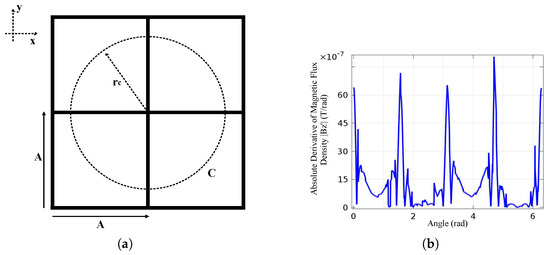
Figure 3.
(a) 3 × 3 m equally spaced square grounding grid configuration. C is the circle with radius equal to on which we take the derivative. (b) 1st order derivative of magnetic flux density on C. Peak at 0 rad corresponds to branch position at , peak at 1.57 rad corresponds to branch position at , peak at 3.14 rad corresponds to branch position at and peak at 4.71 rad corresponds to branch position at . From the location of peaks in Figure 3b, it is determined that grounding grid is lying parallel in the plane of earth as shown in Figure 3a.
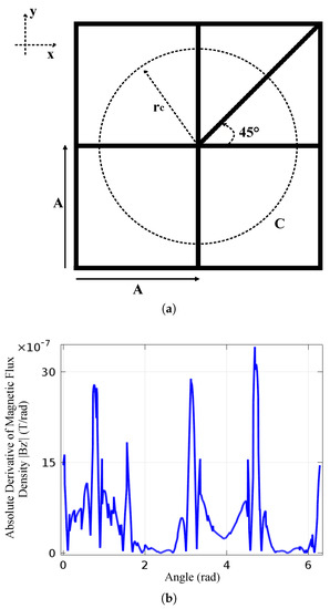
Figure 4.
(a) Equally spaced grounding grid having diagonal branch. The angular displacement between a normal branch and a diagonal branch is . (b) 1st order derivative of magnetic flux density on C. Inter influence sphere (peak width) space between peak at 0 rad, corresponding to branch position at , and peak at 0.78 rad, corresponding to branch position at , has reduced considerably.
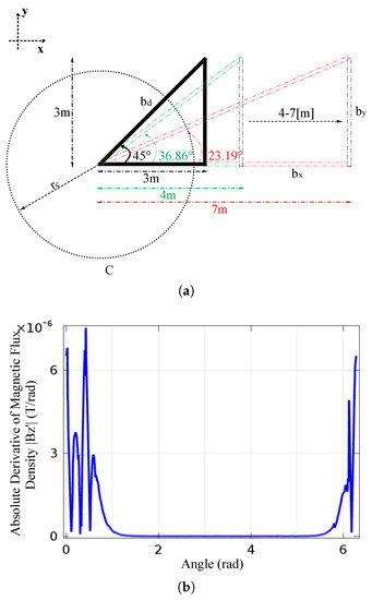
Figure 5.
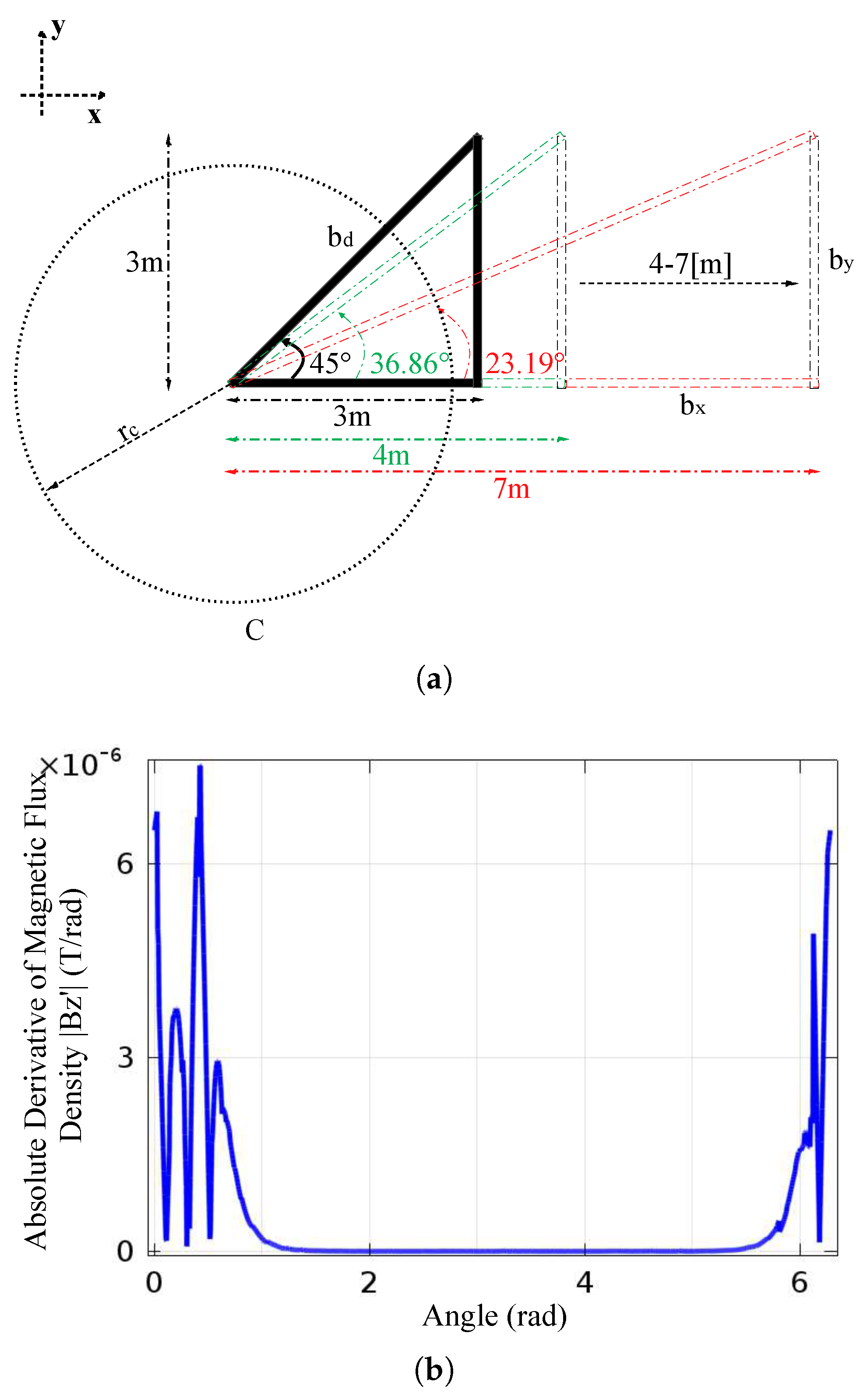
(a) Variation in mesh dimensions: Reduction in angular displacement from to between and , when length of branch is increased from 3 m to 7 m. First order derivative of magnetic flux density is taken on circle C of radius . (b) 1st order derivative on circle C for mesh dimensions 7 × 3 m. Peak at 0 rad corresponds to orientation of , peak at 0.4047 rad corresponds to orientation of , the third peak is a fake which appears due to overlapping of side peaks of and .
Figure 5a illustrates the above problem of unequally spaced grounding grid with a diagonal branch. The angular displacement between ground branches will reduce below and a minimum angular displacement of is encountered in a 7 × 3 m mesh. Our simulation results of a 7 × 3 m grounding grid mesh with a diagonal branch are shown in Figure 5b. Applying the technique in [17] results in overlapping of side peaks of a normal and a diagonal branch. As a result another peak appears, which depicts the presence of an additional ground branch between normal and diagonal branch. The method in [17] fails because there is no branch present between diagonal branch and normal branch as shown in Figure 5a. Therefore, [17] cannot be applied to solve the problem of orientation detection under such circumstances.
In this paper, 3rd order derivative is used to precisely measure the orientation of grounding grid under circumstances for which [17] fails. The reason why 3rd order derivative is used is the reduction in peak width (main peak width plus side peaks width). The main peak width is the width between zero value points of the main peak where side peak width is the width between zero value points of the side peak. This reduction in peak width is understood by analyzing that the derivative is simply the slope of the original signal, means third order derivative is the slope of second order derivative function. Therefore, higher odd derivatives increase the slope of tangent to the curve resulting in sharpening of peak (high resolution) with high peak amplitude and low peak width [18,19].
3. Derivative Method Based Analysis of Current Carrying Buried Conductor
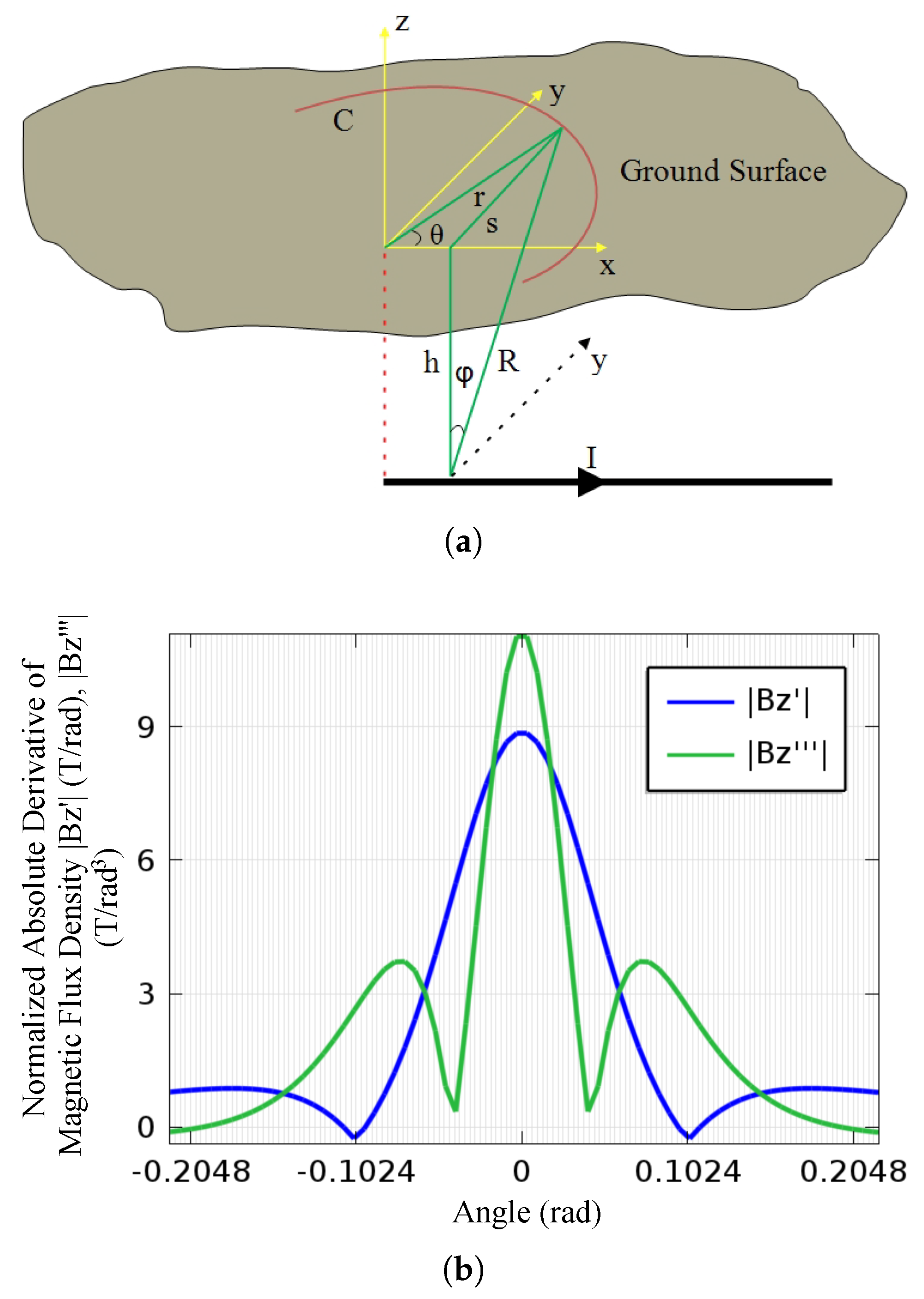
A single current carrying conductor is analysed here for demonstration of the proposed method. Figure 6a shows a conductor of finite length placed along x-axis carrying current I and buried at a depth h below the surface in a mono-layer soil of permeability .
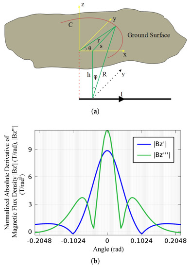
Figure 6.
(a) Single current carrying conductor model: Conductor of finite length along x-axis carrying current I and buried at a depth h below the surface in a mono-layer soil of permeability , derivative of magnetic flux density is taken at the surface of earth on the circle C. (b) 1st and 3rd order circular derivative of magnetic flux density: the position of the main peak is at 0 rad which represents the orientation of buried conductor. Main peak width of is considerably less than the main peak width of and amplitude of is greater than .
According to Ampere’s law, magnetic flux density at the surface is given as:
Putting values from (1–4) into (1), magnetic flux density in z direction is obtained:
Taking the derivative of magnetic flux density on circle C:
Plot of has one main peak and two side peaks as shown in Figure 6b. The main peak is at 0 rad which coincides precisely with orientation of buried conductor.
The width of the peak defines a crucial parameter in determining orientation of grounding grid especially in case where it is unequally spaced. Therefore, width of the peak should be reduced as much as possible. Under worst case conditions as discussed earlier in Section 2, 3rd order derivative is used to determine orientation of grounding grid. By taking 3rd order derivative of , the slope of tangent to the curve increases, resulting in narrowing of peaks as shown in Figure 6b.
The main peak width of can be determined as follows:
From Equation (7), we determine that rad.
In a similar fashion, main peak width of can be determined as follows:
Table 1 summarizes the effect of increasing the order of derivative on the peak width.

Table 1.
Comparison of simulation results between 1st and 3rd order derivative. Keeping depth constant at 0.3m and radius at 2.9 m.
The width of main peaks and side peaks narrows to an extent that it will not overlap and orientation of grounding grid can be easily determined.
4. Simulations and Discussions
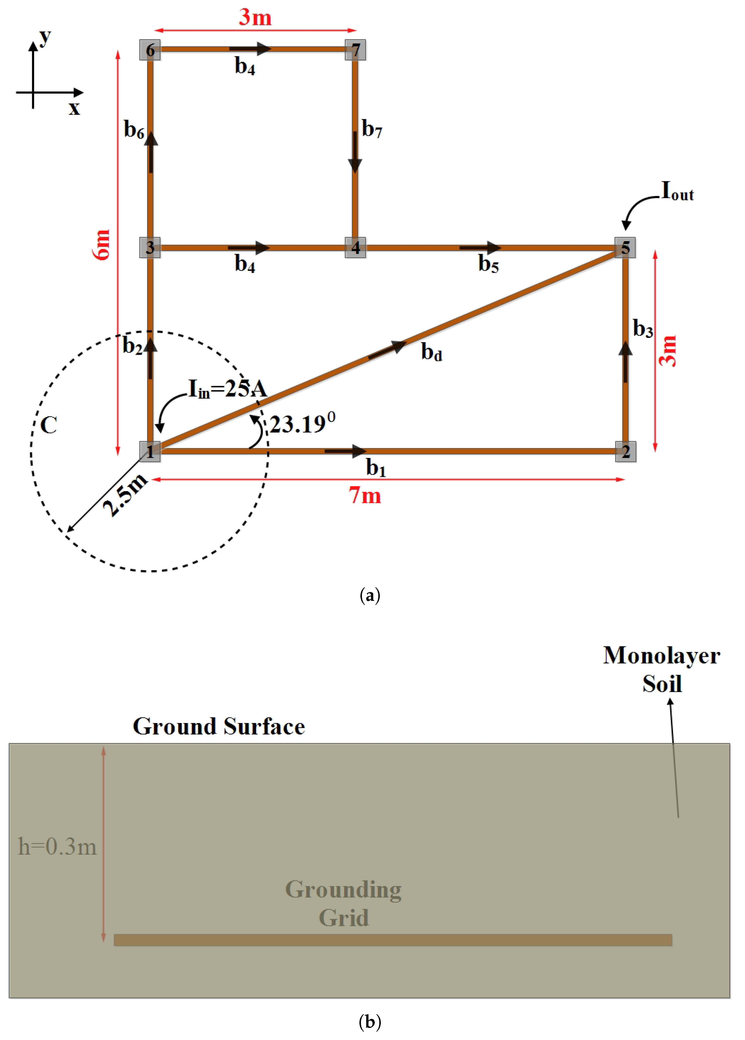
In this section, an unequally spaced grounding grid of dimensions 7 × 6 m is employed for model study. It consists of seven nodes from node 1 to 7 and branches from to made up of copper conductors of radius 0.02 m as shown in Figure 7a. A diagonal branch is also included in the mesh configuration of 7 × 3 m where minimum angular displacement of between diagonal branch and a normal branch is encountered. A dc current of 25A is injected from node 1 and returns at node 5, direction of arrows represents the distribution of current in the grid. The grid is buried in soil at depth of 0.3 m from the surface of earth in a mono-layer soil as shown in Figure 7b. All simulations in this section are carried out using COMSOL Multiphysics 5.0, employing AC/DC module [20].
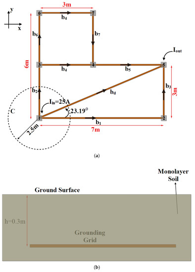
Figure 7.
(a) Simulation model top view: Unequally spaced grounding grid having seven nodes from node 1 to 7 and branches from to made up of copper conductors of radius 0.02 m. A diagonal branch is also included in the mesh configuration of 7 × 3 m where minimum angular displacement of between diagonal branch and a normal branch is encountered. 25A DC current flows into node 1 and returns at node 5 with current distribution as shown. Magnetic flux density is measured along the circle C whose radius is 2.5 m. (b) Simulation model side view: Grounding grid is buried at depth 0.3 m below the earth surface in a monolayer soil.
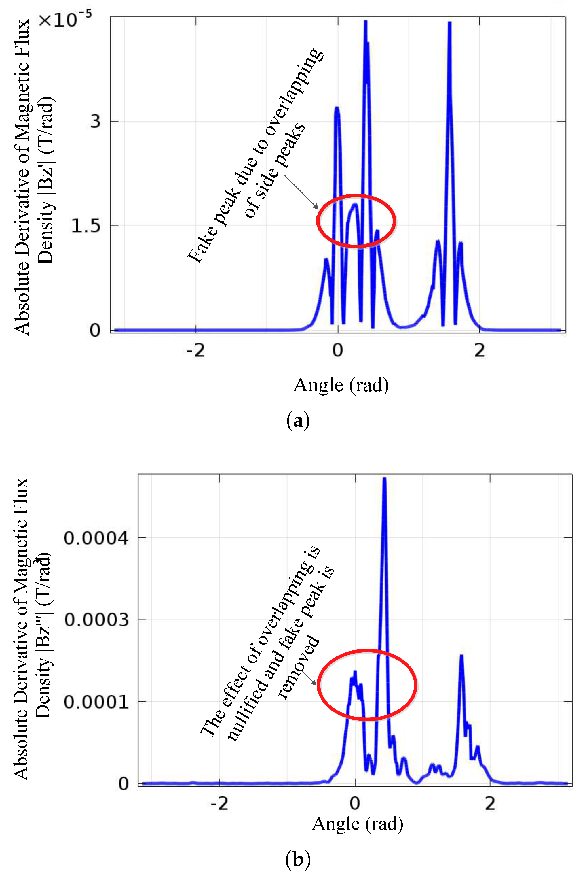
The magnetic flux density on the ground surface in z-direction is . Employing derivative method, 1st order derivative of is taken on the circle C as shown in Figure 8a. Position of peaks in the gradient of represents the orientation of grid conductors. The peak position corresponding to orientation of , and are clearly distinguished at 0 rad, 0.4047 rad and 1.57 rad respectively. A situation of severe ambiguity arises in which a fake peak apparently represents the presence of another branch between and as shown in Figure 8a. However, in contrast this branch does not exist in the grounding grid of Figure 7a. This is because side peaks corresponding to and have overlapped. Due to this overlapping of side peaks, another peak appears between main peaks of and . In order to resolve this ambiguity, 3rd order derivative of is taken where position of peaks represent the orientation of grounding grid as shown in the Figure 8b. The main peak and the side peak width is reduced to an extent that the effect of overlapping is nullified and position of individual peaks can be clearly identified. As a result, position of peaks corresponding to orientation of and are clearly distinguished at 0 rad and 0.4047 rad respectively. The orientation of grounding grid is thus accurately determined which is parallel in the plane of earth.
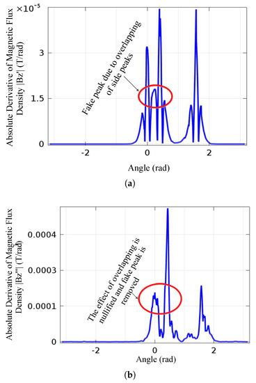
Figure 8.
(a) 1st order derivative of magnetic flux density. Side peaks corresponding to and have overlapped, fake peak appears which represents the presence of another branch between and . (b) 3rd order derivative of magnetic flux density. The main peak and side peak width is reduced to an extent that the effect of overlapping is nullified.
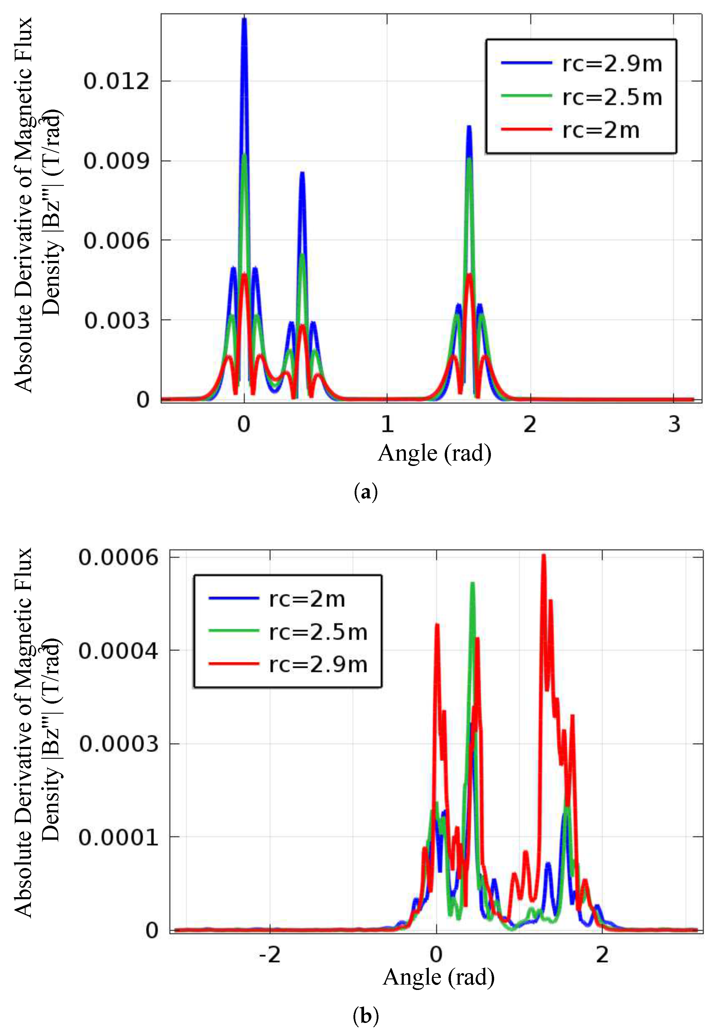
The radius of the circle has inverse relationship with the peak width which is clear from Table 2. The main peak and side peak width will increase with the decrease in radius and vice versa. According to [3] radius r can be chosen between 0 < r < 3 m. Keeping the depth h constant at 0.3 m, it is observed in Figure 9a that the peak width has increased when the radius is reduced from 2.9 m to 2.0 m. Comparing the three simulation results in Figure 9a for 2.9 m , 2.5 m and 2.0 m radius, it can be seen that r = 2.9 m yields best results. The results with r = 2.9 m, has maximum amplitude and minimum peak width among the three results. Hence, peaks obtained with r = 2.9 m are more clear and distinguishable as compared to the other two results. In certain scenarios, the peak width should be kept minimum especially while dealing with grounding grid having minimum angular displacement between adjacent branches. On the other hand, computation points at r = 2.9 m will increase as compared to r = 2.0 m. Therefore, considering the problem scenario, suitable value of radius can be chosen for generating optimised solution. Taking 3rd order derivative adds extra noise due to inherent distortion present in higher order derivatives. Moreover, FEM-based software also has added noise to the results as shown in Figure 9b. However, the noise due higher order derivative can be removed using several regularization techniques such as Total Variation Regularization [21], Tikhonov Regularization [22] and Hybrid Regularization [23].
Table 2.
Comparison of effect on peak width due to varying radius of circle.

Figure 9.
(a) Results with zero noise: Keeping the depth h constant at 0.3 m, 3rd order derivative at = 2.9 m provides best results having maximum peak amplitude and minimum peak width. (b) Results with noise from derivation: 3rd order derivative at = 2.9 m, 2.5 m and 2 m, plot has added noise due to inherent property of derivation and FEM-based software.
5. Conclusions
Practically, a grounding grid with small angular displacement between branches is often encountered. In such situations, the orientation detection technique [17], which is currently employed, fails to deliver accurate results. This is due to overlapping of side peaks corresponding to diagonal and normal branch in a mesh. The 3rd order derivative method presented in this paper effectively resolves this problem that commonly arises in unequally spaced grounding grids. The method eliminates overlapping of side peaks by reducing the peak width even when angular displacement reduces to its critical value of due to the presence of a diagonal branch in the mesh. By the virtue of this method, orientation of all types of grid configuration according to [3] can be precisely determined. Simulation results obtained in this paper illustrate that our method eliminates the overlapping between side peaks corresponding to diagonal and normal branch and peaks are clearly distinguished. The effect of varying radius of circle is also investigated in this paper, which yields fruitful outcomes used for optimizing the solution. Moreover, our proposed method is prone to strong electromagnetic (EMI) environment and therefore, may not produce accurate results under intense EMI. This issue will be addressed in our future research work.
Author Contributions
A.Q. proposed the idea, performed simulations and composed the figures. M.Umair wrote the manuscript. F.Y. did supervision, M.Uzair and Z.K. proof read this work.
Conflicts of Interest
The authors declare no conflict of interest.
Appendix A
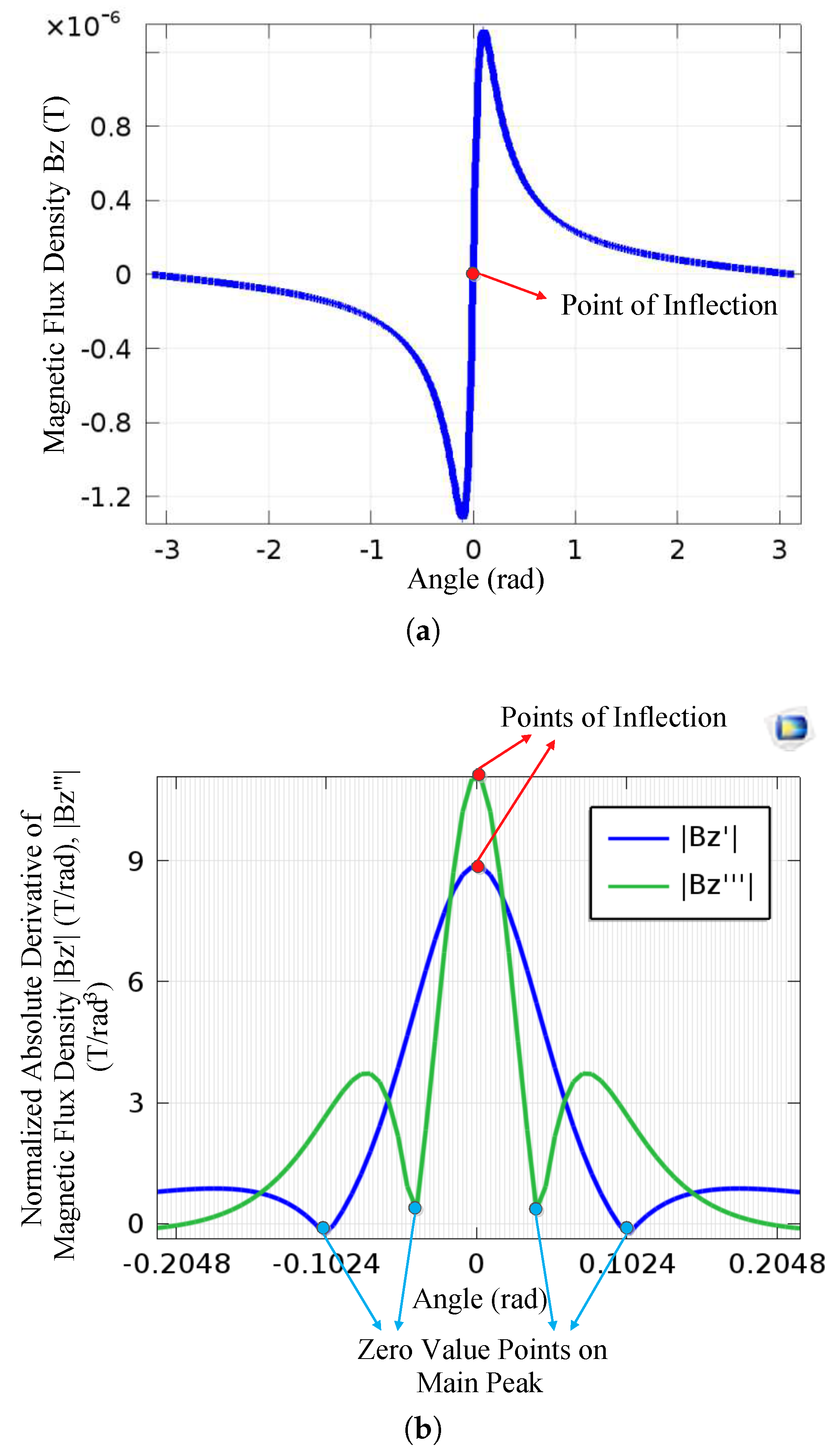
of Equations (7) and (8) demonstrates the width in radians from the point of inflection to the zero value points on the main peak of and . This is shown in the Figure A1. Furthermore, to testify the results mathematically, putting h = 0.3 m and r = 2.9 m that are the considered parameters, from Equation (7) equates 0.103 rad and −0.103 rad and from (8) equates 0.042 rad and −0.042 rad. Analyzing Figure A1b, the location of the main peak zero value points are in close accordance with the mathematical values obtained.

Figure A1.
(a) The magnetic flux density function in (5) has an inflection point at 0 rad, marked as red. (b) Absolute 1st and 3rd order derivative of the function . According to the oscillating behavior of the higher derivatives and absolute values, point of inflection marked as red has the maximum value on the main peak. The points in blue indicate the zero value points on the main peak while the angular width between the zero value points on the main peak is the main peak width.
References
- Rodrigo, A.S.; Akarawita, N.; Ambanwala, A.; Ariyapala, D.; Chaminda, W. Safety in AC substation grounding systems under transient conditions: Development of design software. In Proceedings of the International Conference on Industrial and Information Systems (ICIIS), Peradeniya, Sri Lanka, 17–20 December 2013; pp. 185–190. [Google Scholar]
- Yu, C.; Fu, Z.; Hou, X.; Tai, H.M.; Su, X. Break-point diagnosis of grounding grids using transient electromagnetic apparent resistivity imaging. IEEE Trans. Power Deliv. 2015, 30, 2485–2491. [Google Scholar] [CrossRef]
- Standard, Z.B.O. Guide for Safety in AC Substation Grounding; IEEE Standards Association: Piscataway, NJ, USA, 2006; pp. 80–2000. [Google Scholar]
- Wang, F.; Wang, C. A simulation method on fault diagnosis: Grounding grids. In Proceedings of the International Conference on Advanced Computer Control (ICACC), Shenyang, China, 27–29 March 2010; Volume 1, pp. 207–210. [Google Scholar]
- Zhang, B.; Zhao, Z.; Cui, X.; Li, L. Diagnosis of breaks in substation’s grounding grid by using the electromagnetic method. IEEE Trans. Magn. 2002, 38, 473–476. [Google Scholar] [CrossRef]
- Yu, C.; Fu, Z.; Wang, Q.; Tai, H.M.; Qin, S. A novel method for fault diagnosis of grounding grids. IEEE Trans. Ind. Appl. 2015, 51, 5182–5188. [Google Scholar] [CrossRef]
- Qamar, A.; Shah, N.; Kaleem, Z.; Uddin, Z.; Orakzai, F.A. Breakpoint diagnosis of substation grounding grid using derivative method. Prog. Electromagn. Res. M 2017, 57, 73–80. [Google Scholar] [CrossRef]
- Yang, F.; Wang, Y.; Dong, M.; Kou, X.; Yao, D.; Li, X.; Gao, B.; Ullah, I. A cycle voltage measurement method and application in grounding grids fault location. Energies 2017, 10, 1929. [Google Scholar] [CrossRef]
- Zhang, X.l.; Chen, X. The technique of the optimization applied in the grounding grid’s failure diagnosis. High Volt. Eng. 2000, 26, 64–66. [Google Scholar]
- Wan, X.; Tian, B.; Song, S. Study on the electrochemical sensing system for monitoring/detecting marine steel corrosion. J. Chin. Soc. Corros. Prot. 2009, 21, 182–187. [Google Scholar]
- Hu, X.; Xu, C.; Wang, K. Research on corrosion and protection of grounding grid. Hubei Electr. Power 2002, 26, 75–78. [Google Scholar]
- Xu, G.; Zhu, Z.; Bo, Y. Optimization algorithm of corrosion diagnosis for grounding grid. In Proceedings of the International Conference on Mechanical and Electronics Engineering (ICMEE), Kyoto, Japan, 1–3 August 2010; Volume 2, pp. 2–42. [Google Scholar]
- Qiu, Q.r.; Wang, P. A new optimization algorithm for grounding grid fault diagnosis. In Proceedings of the International Workshop on Modelling, Simulation and Optimization, Hong Kong, China, 28 December 2008; pp. 294–297. [Google Scholar]
- Liu, Y.; Xu, X.; Li, L.; Tan, S. Reconstruction of substation grounding grid based on concept of regret. In Proceedings of the International Conference on High Voltage Engineering and Application (ICHVE), Chengdu, China, 19–22 September 2016; pp. 1–4. [Google Scholar]
- Yu, C.; Fu, Z.; Wu, G.; Zhou, L.; Zhu, X.; Bao, M. Configuration detection of substation grounding grid using transient electromagnetic method. IEEE Trans. Ind. Electron. 2017, 64, 6475–6483. [Google Scholar] [CrossRef]
- Chunli, L.; Wei, H.; Degui, Y.; Fan, Y.; Xiaokuo, K.; Xiaoyu, W. Topological measurement and characterization of substation grounding grids based on derivative method. Int. J. Electr. Energy Syst. 2014, 63, 158–164. [Google Scholar] [CrossRef]
- Qamar, A.; Yang, F.; He, W.; Jadoon, A.; Khan, M.Z.; Xu, N. Topology measurement of substation’s grounding grid by using electromagnetic and derivative method. Prog. Electromagn. Res. B 2016, 67, 71–90. [Google Scholar] [CrossRef]
- Yang, F.; Liu, K.; Zhu, L.; Zhang, S.; Hu, J.; Wang, X.; Gao, B. A derivative-based method for buried depth detection of metal conductors. IEEE Trans. Magn. 2018, 54, 1–9. [Google Scholar]
- Cuellar, R.E.; Ford, G.A.; Briggs, W.R.; Thompson, W.F. Application of higher derivative techniques to analysis of high-resolution thermal denaturation profiles of reassociated repetitive DNA. Proc. Natl. Acad. Sci. USA 1978, 75, 6026–6030. [Google Scholar] [CrossRef] [PubMed]
- AC/DC Module User’s Guide, Version 5.0, COMSOL, Inc. Available online: www.comsol.com (accessed on 18 December 2017).
- Ahnert, K.; Abel, M. Numerical differentiation of experimental data: Local versus global methods. Comput. Phys. Commun. 2007, 177, 764–774. [Google Scholar] [CrossRef]
- Lubansky, A.; Yeow, Y.L.; Leong, Y.K.; Wickramasinghe, S.R.; Han, B. A general method of computing the derivative of experimental data. AIChE J. 2006, 52, 323–332. [Google Scholar] [CrossRef]
- Song, X.; Xu, Y.; Dong, F. A hybrid regularization method combining Tikhonov with total variation for electrical resistance tomography. Flow Meas. Instrum. 2015, 46, 268–275. [Google Scholar] [CrossRef]


© 2018 by the authors. Licensee MDPI, Basel, Switzerland. This article is an open access article distributed under the terms and conditions of the Creative Commons Attribution (CC BY) license (http://creativecommons.org/licenses/by/4.0/).