The above-mentioned horizontal comparison process combines the operating conditions of multiple units, which can effectively avoid the abnormal alarm caused by the active power change of the wind turbine caused by accidental reasons. For example, in the weather with high wind speed, the power generation capacity of the unit is generally higher than before. By comparing the operating parameters between the units, the cause of the alarm can be identified. However, the horizontal comparison can only roughly judge whether the current state is abnormal through Real-time data, and the fault warning needs to be implemented in combination with an effective modeling method.
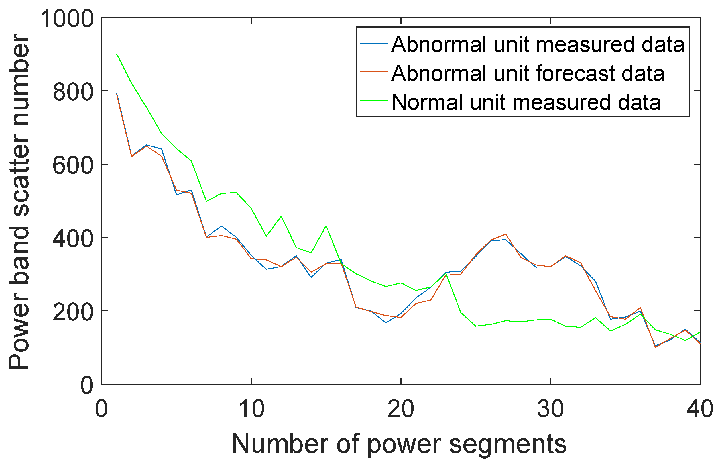
This chapter introduces the idea of deep learning into the neural network by modeling the single unit and using historical data as a training sample. Through the convolution operation to extract different levels of features from shallow to deep, the neural network training process is used to make the whole network automatically adjust the parameters of the convolution kernel, so that the most suitable classification features are generated unsupervised, and the above process is assisted in state judgment. While training the historical normal operation data and the reliable data of the relevant units, this model can predict the scatter distribution of the unit components in a short period of time, which can play a good role.
4.1. Convolutional Neural Network Structure
To establish the gearbox temperature CNN model, it is necessary to determine the modeling variables in the training sample, which are closely related to the gearbox bearing temperature. Through the analysis of 40 parameters of 1-min class recorded by the SCADA system, 5 variables of active power, wind speed, ambient temperature, cabin temperature and gearbox oil temperature closely related to bearing temperature are selected as inputs, and the gearbox bearing temperature is used as the output.
For the input of the convolutional neural network in this paper, the method of selecting variables is based on the Expert Evaluation method and Partial Least Squares (PLS) method.The wealth of experience and breadth of knowledge of experts provides a reference value for the initial selection of variables. The PLS method is an applied statistical method that integrates the basic functions of multivariate statistical regression, canonical correlation analysis and Principal Component Analysis (PCA). This method can select the combination of independent variables with the largest correlation with the dependent variable, and solve the multiple correlation of variables in the regression analysis. The extracted principal components are well interpreted and can eliminate correlation between multiple variables. As shown below:
(1) Active power (P): It is closely related to the gearbox temperature. When the output power of the unit is high, the load on the gearbox is large, resulting in high gearbox temperature.
(2) Wind speed (u): Wind is the source of energy for wind turbines. For the variable speed wind turbines studied in this paper, the speed of the transmission system is proportional to the wind speed for the purpose of achieving the best tip speed ratio for maximum wind energy tracking. The higher the wind speed, the higher the gearbox speed, which causes the gearbox temperature to rise.
(3) Ambient temperature (T): Since the ambient temperature of the unit varies greatly in the short-term (day and night) and long-term (week, month) time scales, the ambient temperature must be considered as one of the factors. Especially in the spring of March and April, due to the wind and cold, the ambient temperature difference can reach 30 C. At different times, even if the power and wind speed of the unit are the same, the temperature of the gearbox will vary greatly due to the difference in ambient temperature.
(4) Cabin temperature (T1): Due to uneven distribution of temperature field inside the wind turbine cabin, it will cause the main heat source inside the engine room (such as generator, gear box, etc.) to stop due to over temperature alarm.
(5) Gearbox oil temperature (T2): The oil temperature of the gearbox is too high, which will cause the fan to stop, and has a serious impact on the power generation.
At the same time, because the gearbox bearing temperature parameter changes have a large inertia, the gearbox temperature at the previous moment has a direct impact on the current temperature. Thus, six adjacent historical moments are selected as a set of samples.The training samples included a total of 14,000 samples from May 1 to June 30, each of which is a 6 × 6 vector. The vector contains 6 sets of data of 6 variables adjacent to each other at the historical moment. Since the convolutional neural network is a multi-level neural network, it includes a filtering level and a classification level. The filtering stage is used to extract the characteristics of the input signal, and the classification level classifies the learned features, and the two-level network parameters are jointly trained. The filtering stage consists of three basic units: a convolutional layer, a pooled layer and an active layer. The classification level is generally composed of a fully connected layer.
(1) Convolution layer
The convolutional layer uses a convolutional kernel to perform convolution on the local area of the input signal (or feature) and produces corresponding features. The most important feature is weight sharing, in which the same convolution kernel traverses input once in fixed steps. Weight sharing reduces the network parameters of the convolutional layer, and avoids overfitting due to excessive parameters, and reduces system memory requirements. In practice, correlation operations are mostly used instead of convolution operations to avoid flipping the convolution kernel when back propagation happens. The concrete convolutional layer operation is shown in Equation (
14).
—the weight of the i convolution kernel of layer l
—the jth convolved local area in layer l
w—the width of the convolution kernel
When one-dimensional convolutional layer operations are performed, each convolution kernel traverses the convolutional layer once and performs convolution operation at the same time. Take the first convolution kernel as an example. In the convolution operation, the nucleus multiplies the coefficients corresponding to the neurons in the volume area, then moves the convolution kernel in steps of 1 and repeats the previous operation until the volume. The nucleus traverses all areas of the input signal.
(2) Activation layer
After the active layer is convolved, the activation function will nonlinearly transform the logits value of each convolution output. The purpose of the activation function is to map the linearly inseparable multidimensional features to another space. Since the ReLU (Rectified Linear Unit) function always has a derivative value of 1 when the input value is greater than 0, the gradient diffusion phenomenon is easy to overcome. Therefore, ReLU is used as the activation function of the convolutional neural network. The ReLU function is as follows.
—the activation value of the convolutional output
(3) Pooling layer
The pooling operation downsamples the width and depth of the original feature to the output by adjusting the size and step size. The downsampling operation used in this paper is a maximum pooling. It takes the maximum value in the sensing domain as an output, and the advantage of that is it can obtain position-independent features that are critical for periodic time-domain signals.
—the activation value of the t neuron in the i layer of the l layer
—the width of the pooled area
(4) Fully connected layer
The fully connected layer classifies the features extracted by the filter stage. The specific approach is to first spread the output of the last pooling layer into a one-dimensional feature vector as the input of the full-connected layer; then to fully connect the input and output, in which ReLU is used as the activation function of hidden layer. The last output layer’s activation function is Softmax.
—the weight between the i neuron in the l layer and the j neuron in the layer
—the bias value of the j neuron in the layer for all neurons in the l layer
(5) Objective function
The output of the segment input signal in the neural network should be consistent with its target value. The function to evaluate this consistency is called the objective function of the neural network. The commonly used objective function has a squared error function and a cross entropy loss function. The actual output of the convolutional neural network has a Softmax value of
q, and its target distribution
p is a one-hot type vector. That is, when the target category is
j,
, otherwise 0.
Compared with the squared error function, the cross entropy function measures the consistency of the two probability distributions. The cross entropy function is often regarded as the negative log likelihood of the Softmax distribution in machine learning, so the cross entropy function is used as the objective function in this paper. The network consists of two convolutional layers, two pooling layers, a fully connected hidden layer, and a Softmax layer.
4.2. Convolutional Neural Network Error Back Propagation
Error backpropagation is a key step in weight optimization for neural networks. The main method is to solve the derivative function of the objective function with respect to the last layer of neurons. Through the chain rule, the derivative value of the objective function with respect to the ownership value is calculated layer by layer from the back to the front.
(1) Full connection layer reverse derivation
First, calculate the derivative of the objective function
L about the last level of the logits value
.
Then calculate the derivative
of the objective function
L of the fully connected layer and the derivative of the offset
.
Finally, the objective function
L is calculated. The activation value
of the fully connected hidden layer whose activation function is ReLU and the derivative of the logits value
.
(2) Pooled layer reverse derivation
After the value is calculated by the above formula, the objective function L is continuously solved for the derivative of the weight of the fully connected hidden layer and the bias term . When the objective function L is solved for the logits value of the fully connected layer and the derivative of the weight, then the derivative of each parameter of the pooling layer is calculated. Since the pooling layer has no weight, it is only necessary to calculate the derivative of the input neurons of the pooling layer.
The specific practice for pooling the maximum value is: record the maximum position of the pooled area during forward propagation. When
t=
,
. In the case of backpropagation, the derivative value is passed to the
neuron, and the other neurons do not participate in the transmission, which the derivative is zero.
(3) Convolutional layer reverse derivation
First, calculate the derivative of
L’s logits value for each convolutional layer, since the convolutional layer uses the ReLU activation function.
Next, calculate the derivative of
L about the input value
of the convolutional layer.
Finally, calculate the derivative of
L on the convolution kernel
.
(4) Adam optimization algorithm
After calculating the derivative of each weight of the objective function by using the error back propagation algorithm, the next step is to use the optimization algorithm to update the weight. Solve the optimal weight, so that the value of the objective function is minimized. This process is described by the following formula:
,—objective function value and output value
—all parameters of the convolutional neural network
—the optimal parameter of the convolutional neural network
—input of the convolutional neural network
For shallow neural networks, the use of stochastic gradient-decreasing (SGD), which is widely used in BP neural networks, can converge to the global. However, for the deep convolutional neural network proposed in this chapter, due to the large number of parameters and hyperparameters, if the superparameter selection is not good, the use of SGD training tends to fall into the local best. Therefore, the Adam algorithm is used in this paper. Adam is a learning rate adaptive optimization algorithm that dynamically adjusts the learning rate of each parameter by using the first moment estimation and the second moment estimation of the gradient. Adam’s advantage lies in the correction of the first moment and non-central second moment of the initialization from the origin after offset correction, so that each iteration learning rate has a certain range. Adam is generally robust to the selection of multiple parameters and therefore helps in parameter adjustment of the neural network.


