Abstract
Utility harmonic impedance is an important parameter for harmonic mitigation. In this paper, a method for utility harmonic impedance estimation method based on constrained independent component analysis is proposed. The conventional impedance estimation method based on ComplexICA has two major problems: the algorithm is not suitable for separating weak and strong source mixed signals, and lots of sample data should be provided to avoid converging on a local optimum. To solve the two problems, the prior information of the utility harmonic source is added to the objective function of ComplexICA; in this paper, the measurement data at PCC when the load is shutdown are chosen as the prior information. Then the utility harmonic source signal can be recovered and the separated matrix can be obtained effectively. The connection between the utility harmonic source, utility harmonic impedance and the data at PCC are established using Norton equivalent circuit, and then the separation matrix is used to calculate utility harmonic impedance. The performance and feasibility of the proposed method are verified by the computer simulation and field test. Compared with the current ComplexICA method, the proposed method is more adaptive to changes in the background harmonic and the calculation result is more stable.
1. Introduction
With the proliferation of power systems, more and more non-linear loads are connected to the grid, which results in harmonic distortion and increases the harmonic voltage and current levels. Limiting harmonic emissions from customer facilities has become a common industry practice. IEEE Std.519 [1] and IEC61000-3-6 [2] have governed the harmonic voltage and current a customer facility can inject into the supply power system. The standards are used during both the facility planning stage and the operation stage, and the harmonic emission level of customer facility should be calculated to check whether it is exceeding the planning level [3]. However, it is difficult because the harmonic distortion measured at PCC (the point of common coupling, PCC) is caused by both the customer facility and the supply system. Unfortunately, there is still no effective method to determine a customer’s contribution to the harmonic distortions measured at PCC.
Many studies have been conducted to determine customers’ harmonic contribution; the Norton equivalent circuit is usually adopted, and the key parameter in the equivalent circuit to estimate harmonic contribution is the utility harmonic impedance [4]. Therefore, in recent years, many studies have been focused on the estimation of utility harmonic impedance, which can be divided into invasive methods [5,6,7,8,9,10] and non-invasive methods [11,12,13,14,15,16,17,18,19,20,21,22]. Invasive methods intend to create a disturbance in power system, and then measure the responses of harmonic voltage and current at PCC. The results of invasive methods are often more reliable than those of non-invasive methods [17]. However, the disturbance has a large impact on the network so that the supply side may not permit such an experiment. Furthermore, invasive methods are often difficult to perform due to the cost of the equipment used to make the disturbance [17,22].
The non-invasive methods, in contrast, obtain utility harmonic impedance information using the natural variations of the harmonic current and voltage at PCC [21,22], and the proper data for non-invasive methods are easy to obtain from the power quality monitor. Several non-invasive methods for utility harmonic impedance estimation have been proposed. For example, in fluctuation methods [11,12], the utility harmonic impedance is quantified using the ratio of harmonic voltage fluctuation and harmonic current fluctuation. The selection of fluctuation data only caused by the customer side is the key to this method, but in practice, utility side and customer side often fluctuate simultaneously.
In the linear regressive method [13,14,15], the utility harmonic impedance is calculated by solving the coefficients of the equivalent circuit equation using the regression algorithm. In [16], based on the covariance characteristic of the random vector, i.e., when the covariance between independent vectors is 0, a method is proposed to calculate the utility harmonic impedance. These methods are sensitive to the background harmonic voltage fluctuation: when there is a large fluctuation in the background harmonic voltage, neither the regressive method nor the covariance method are effective.
In the method based on data selection [12,17,18,19], the critical point of these methods is selecting the harmonic voltage and current fluctuation only caused by the customer side. However, utility side and customer side usually fluctuate at the same time, so it is difficult to select the proper data used for utility harmonic impedance estimation when the background harmonic fluctuates wildly.
In [23], the author indicated that harmonic loads fluctuation can be divided into slow-varying components and fast-varying components using a linear filter, and the fast-varying components of loads are statistically independent and have non-Gaussian distribution. Based on these principles, in [21,22], utility harmonic impedance estimation methods based on independent component analysis have been proposed. These methods are more robust to the fluctuation of background harmonic voltage. However, there are two problems with the independent component analysis. The first is that the basic theory of the independent component analysis is Central Limit Theorem [24], when the mean and variance of the source signals are not of the same order of magnitude; in other words, the source signal dominates the mixed signal, so the source signals do not satisfy this theorem and the independent component analysis is not suitable for signal separation. In a power system, this occurs when the utility harmonic source is much smaller than the customer harmonic source; in this situation, the ICA method will be invalid. The second problem is that the traditional independent component analysis can easily fall into a local optimum, so that long-term data should be provided to obtain reliable calculation results, which means the calculation amount of the algorithm is large and it is difficult to obtain real-time harmonic impedance information.
In this paper, based on complex constrained independent component analysis (ComplexCICA), a method is proposed to estimate the utility harmonic impedance, which can solve the two existing problems with the ICA method. The main steps of the proposed method are as follows. First, the prior information of the utility harmonic source is added to the objective function of classical complex independent component analysis, and the PCC data are applied in the proposed algorithm to obtain the separated matrix. Secondly, the relationship matrix between the PCC harmonic data and the utility harmonic source are built based on the Norton equivalent circuit. Finally, when we compare the relationship matrix and the separated matrix, the utility harmonic impedance is then calculated out. This paper is organized as follows. Section 2 describes the basic principles of the utility harmonic impedance estimation, the weakness of the ComplexICA algorithm, and the principle of the constrained ICA algorithm. The proposed utility harmonic impedance estimation method is explained in Section 3. The performance of the proposed method is certified with the computer simulation and the field test in Section 4. In Section 5, some conclusions about the proposed method are summarized.
2. Basic Principles
A common case for utility harmonic impedance estimation is shown in Figure 1. The interface point between the utility and customer facilities is called PCC. The revenue meters or power quality monitors are usually connected at the interface, so the data for non-invasive utility harmonic impedance estimation can be recorded in the meter.
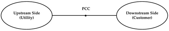
Figure 1.
Equivalent interpretation of distribution system at the PCC.
2.1. Equivalent Model for Utility Harmonic Impedance Estimation
In this paper, the utility side and customer side are modeled using a Norton equivalent circuit as shown in Figure 2:
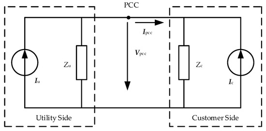
Figure 2.
Norton equivalent circuit.
where Iu and Ic are the harmonic current sources of utility and customer, respectively; Zu and Zc are the harmonic impedances of utility and customer, respectively; Vpcc and Ipcc are the recorded harmonic voltage and current data at PCC, respectively. The equivalent circuit is suitable for different frequencies, where the parameters in the circuit will be different.
According to the equivalent circuit and superposition theorem, the equation of the circuit can be established as follows:
Because the variations of Iu are related to the harmonic loads connected to the utility side, and the variations of Ic are related to the harmonic loads connected to the customer side, the features of the harmonic source are same as the harmonic loads. The Iu and Ic can be divided into a fast-varying component and a slow-varying component by utilizing a linear filter [23]. The fast-varying components are considered statistically independent and have non-Gaussian distribution. The measurement harmonic voltage Vpcc and current Ipcc data at PCC are the linear combination of the harmonic source, which can be divided into a fast-varying component and a slow-varying component by utilizing a linear filter too. Therefore, the independent component analysis algorithm can be applied to the fast-varying component of the data at the PCC. Equation (1) can be expressed as:
where “Δ” represents the fast-varying component of the harmonic signal.
2.2. The Weakness of the ComplexICA Algorithm for Separating Weak Signal
According to the Lindeberg–Feller Central Limit Theorem [25], suppose that are the random series that the mean is and the variance is , and the partial sum of the series is defined as:
For each , if the sequence satisfies Equation (4), and , based on the Lindeberg–Feller condition, the sequences that accord with the condition have normal distribution, expressed as . In fact, the Lindeberg–Feller condition is the necessary and sufficient condition for sequences that have normal distribution.
The essence of the theorem is that the mean and the variance of the source signal that compose the mixed signal should be on the same order of magnitude, which requires that every source signal should not dominate the mixed signal. In other words, mixed signals, which are composed of weak and strong source signals, will not accord with the Central Limit Theorem. However, the ComplexICA algorithm is based on the Central Limit Theorem [24], which indicates that the algorithm is not suitable for extracting the weak signal from a mixed signal that is composed of a weak and strong source signal.
To verify the viewpoint, a simple experiment is carried out using Matlab. Three source signals with different magnitude are generated in Matlab. As shown in Figure 3(a1,b1,c1), the first source signal is a Laplace distribution random variable, Lap (0, 50). The second source signal is an equal amplitude triangle signal. The third source signal is a sinusoidal signal. As shown in Figure 3(a1,b1, c1), the magnitude of the three source signals is different. In this experiment, the first signal is generated as the strong signal, and the second and third signals represent weak signals. Then the three source signals are mixed using a random matrix; the mixed signals are shown in Figure 3(a2, b2,c2). Finally, the separated signals or recovered signals are obtained by applying the ComplexICA algorithm to the mixed signals; the separated signals are shown in Figure 3(a3,b3,c3).
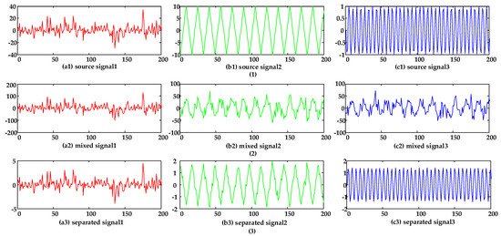
Figure 3.
(a1) The waveform of the first source signals; (b1) The waveform of the second source signals; (c1) The waveform of the third source signals; (a2) The waveform of the first mixed signals; (b2) The waveform of the second mixed signals; (c2) The waveform of the third mixed signals; (a3) The waveform of the first separated signals; (b3) The waveform of the second separated signals; (c3) The waveform of the third separated signals.
Comparing Figure 3(a1) and Figure 3(a2,b2,c2), the waveforms of the mixed signals are similar to the first source signal, which means that the strong signal is dominant to the mixed signal. From the waveforms of the source signals and the separated signals in Figure 3(a1,a3), it can be seen that the first separated signal is the same as the first source signal except for the shrinking of the scale. However, comparing Figure 3(b1) with Figure 3(b3), the magnitudes of the second separated signal are not equal to each other and there are some waveform distortions in the second separated signal, which are different to the second source signal. The results of the experiment indicate that the ComplexICA algorithm is not suitable for separating mixed signals whose magnitudes are not of the same order. In this condition, the statistical characteristics of the weak signal are masked by the strong signal, so the strong signal plays a dominant role in the mixed signals, which is not in accordance with the Lindeberg–Feller Central Limit Theorem. Therefore, the ComplexICA algorithm based on the Central Limit Theorem is not suitable for separating the weak signal from a mixed signal.
2.3. The Constrained Complex Independent Component Analysis
First, the basic principle of independent component analysis is presented. ICA is a main algorithm in the blind separation problem. The source signal can be recovered from the mixed signal or observed signal by applying the ICA without the information of the mixed matrix [22]. The ICA model is expressed as follows:
where X is the observed signal, in this paper, which represents the measurement data at PCC; A is the mixed matrix; and S is the source signal, which represents the utility and utility harmonic source. In the ICA model, X and A are unknown; the goal of the algorithm is obtained from the separated matrix and then we estimate the source signal by Equation (6):
where is the estimated source signal and W is the separated matrix. The model of the constrained independent component analysis is the same as for the ICA.
The constrained independent component analysis was first proposed in [26], in this paper, the author solved the indeterminacy problems in traditional ICA algorithm. The principle of CICA (constrained independent component analysis) is adding the additional requirement or the available prior information of the target signal into the classical ICA contrast function in the form of equality or inequality constraints, so the target signal is separated firstly. In this paper, the CICA algorithm is realized by Non-Gaussian Maximization; the entropy is usually used to measure the non-Gaussian according to the information theory. The approach of the CICA algorithm in this paper can be expressed as follows:
First, define the negative entropy approximation function:
where y is the subject separated signal; is a constant value, which is used to adjust the step of the algorithm, in this paper, the value is 1; represents the mean of ‘’, v is a Gaussian variable whose mean is 0 and variance is 1; and is a non-quadratic function, e.g., , , in this paper, the second function is chosen.
Next, define the similarity measure : when the separated signal approximates the target signal, the measure has the minimum value. The measure is usually represented by mean square error norm, as follows:
where r is the reference vector of the target signal, which includes the prior information of the source signal.
Then, the CICA algorithm can be expressed as:
where w is the row of the separated matrix W and is the threshold used to distinguish the specific source signal; in this paper, the value is 0.5.
By applying the Lagrange multiplier method, the objective function can be solved. First, convert the inequality constraints into equality constraints by employing the relaxation factor “Z”, then Equation (7) can be expressed as:
where is the Lagrangian multiplier; is the scalar processing function—in this paper, the value is 1; and Z is the relaxation factor.
Then, is calculated by applying the quasi-Newton iteration method:
where k is iteration; is the learning efficiency; is the first derivation of the Lagrange function versus the w; and are the first derivation and second derivation of versus y, respectively; and and are the first derivation and second derivation of versus y, respectively.
The principle diagram of the CICA is shown in Figure 4. In the CICA algorithm, the independence of the separated signals is measured by the negative entropy, which is similar to the classical ComplexICA algorithm. However, there are still some differences between the two algorithms; for example, in the ComplexICA algorithm, the signal that has the largest entropy is extracted first. However, in the CICA algorithm, the target separated signal will have the largest negative entropy due to introducing the reference vector that includes the information of the target signal, so that the target signal can be separated first. At the same time, compared with the classical algorithm, the algorithm can obtain the global optimum, rather than the local optimum, so a more stable calculation result can be obtained. However, the proposed algorithm can reduce the iteration times by introducing the reference vector, so the calculation speed and performance of the algorithm can be improved.
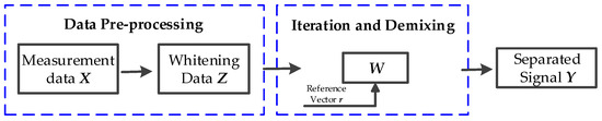
Figure 4.
Principle diagram of the constrained independent component analysis algorithm.
3. Proposed Method
In a power system, the utility harmonic source fluctuation is usually smaller than the customer side. In Section 2.2, the classical ComplexICA algorithm indicated is not suitable for extracting the weak signal in the measurement data; therefore, the utility harmonic impedance estimation method based on ComplexICA is not correct in some cases. What is more, because there is no prior information used in the traditional algorithm, there is some indeterminacy in the separation results. Finally, with the classical algorithm it is easy to final the local optimum, but a large amount of measurement data is required to get a more reliable result, which means the real-time harmonic impedance data cannot be obtained effectively.
In this paper, a utility harmonic impedance estimation method based on the ComplexCICA is proposed. The measurement harmonic voltage and current data when the load is shutdown are selected as the prior information of the utility harmonic source, which is the reference vector of the ComplexCICA. Then the ComplexCICA algorithm is applied to the measurement harmonic voltage and current data, and the utility harmonic source and the separated matrix are separated. The relationship between the utility harmonic source and harmonic voltage and current at PCC is deduced through the Norton equivalent circuit in Figure 2. Finally, the utility harmonic impedance is calculated by comparing the separated matrix and the relationship matrix.
According to the Norton equivalent circuit, Equation (2) can be expressed as a matrix:
Then extract the inverse matrix of Equation (12):
The relationship between the utility harmonic signal and the harmonic voltage and current data at PCC is as shown in Equation (11), and the scale indetermination problem of classical ICA can be solved utilizing Equation (13), too. Assume that the separated signal is k times the real utility harmonic source signal, as follows:
where is the separated signal by using the ComplexCICA algorithm and is the real utility harmonic signal.
The separated matrix of utility side is as follows:
where U is the separated matrix by using the ComplexCICA algorithm; is k times to the ; is equal to k in value.
Based on Equations (13), (14), and (16), the relationship between , and can be expressed as follows:
Comparing Equations (13) and (17), the utility harmonic impedance can be calculated by:
Then the proposed utility harmonic impedance estimation method based on the ComplexCICA method is completed. The flow diagram of the proposed method is shown in Figure 5.
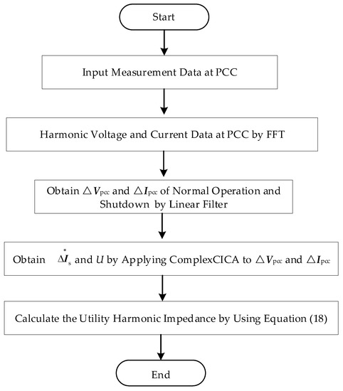
Figure 5.
Flow diagram of the proposed method.
With the development of the power system and power electronic technology, lots of distributed generators are connected to the power system, like solar and wind power; therefore, the hybrid AC/DC microgrids have become a trend in future power systems. These microgrids have two subgrids linked to each other where the AC subgrid can connect to the utility grid [27,28] and the loads obtain power from both utility and customer. One of the technical challenges regarding power quality in hybrid AC/DC microgrids is the difficulty of harmonic analysis. These grids are not the same as the traditional power system; because of the effect of the filters that connect the distributed generators and power system, the customer harmonic impedance will not be considerably larger than the utility side. Therefore, the traditional harmonic impedance estimation methods based on this assumption will be invalid. The proposed method is not based on this assumption, which may be useful for harmonic analysis in these microgrids.
4. Simulation
The performance of the proposed method is verified by computer simulation and field testing in this section.
4.1. Computer Simulation
In this part, the circuit model presented in Figure 2 is simulated in Matlab/Simulink. The slow-varying component of the utility and customer harmonic source are modeled with the typical load curve in [22], and the fast-varying component of the customer harmonic source is modeled with the Laplace distribution random variable Lap (a, b) with expectation a and variance b. The fast-varying component of the utility side is k times that of the customer side. The customer harmonic impedance is p times that of the utility side. The specific parameters of source and impedance are shown in Table 1.

Table 1.
Parameters for simulation model.
In the simulation, k represents the fluctuation degree of Iu relative to Ic, and p represents the different magnitude of Zc relative to Zu. In an entire day, there are 1440 samples (one point per minute) at PCC; the sample data are separated to obtain the fast-varying component of Ipcc and Vpcc by utilizing a linear filter. In this paper, two utility harmonic impedance estimation methods are compared. Method 1 is the method based on ComplexICA [22] and Method 2 is the method proposed in this paper. Figure 6 shows the magnitude of harmonic current and voltage at PCC when k = 0.2, p = 10.
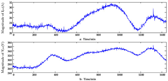
Figure 6.
(a) The waveform of the harmonic current at PCC (k = 0.2, p = 10); (b) The waveform of the harmonic voltage at PCC (k = 0.2, p = 10).
When p = 10, for different k, which represent different fluctuations of Iu, the two different methods are used to calculate the utility harmonic impedance. The errors of the imaginary parts and the real parts of the calculated Zu are shown in Table 2. According to the results, with the fluctuation of the background harmonic, the accuracy of Method 1 is changing constantly, and the estimation errors are changing for different k. In contrast, the estimation error of the proposed method is smaller than in Method 1, although the error also fluctuates with k, which means that the proposed method is more robust to the fluctuation of the background harmonic.
Table 2.
Errors of two methods for different k.
The adaptability of the proposed method for different p is illustrated in the next simulation. When k = 0.2, and p varies from 1 to 15, the utility harmonic impedance is calculated by utilizing the two methods. The errors of the imaginary and real parts of the impedance are shown in Table 3. Based on Table 3, when the fluctuation of the background harmonic is constant, the estimation errors of the two methods are nearly invariant for different p. Even though the estimation errors are nearly constant, the errors of the proposed method are smaller than for Method 1. In other words, the proposed method is more adaptable to changes in the magnitude ratio of Zu relative to Zc.
Table 3.
Errors of two methods for different p.
The estimation errors of the two methods for different k and different p are shown in Figure 7, where the adaptability of the two methods can be observed more intuitively. Based on Figure 7, we see that when p is constant, k varies from 0.1 to 1.5; the estimation errors of Method 1 fluctuate with the variation of k, and the estimation errors are smaller when k is in the range of 0.5 to 1, which accords with the conclusion that the classical ICA method is only suitable for separating mixed signals with similar amplitude. For the proposed method, except for a few points, the estimation error is smaller in most cases. When k is constant, p varies from 1 to 15; the estimation errors of each method are nearly constant, which means that the estimation results are not sensitive to the different magnitude of Zu relative to Zc, and the errors of the proposed method are smaller than in Method 1. In conclusion, the proposed method is more robust to the fluctuation of the background and the different magnitude ratio of impedance.
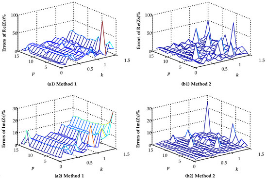
Figure 7.
(a1) Errors of impedance-real part for method 1; (a2) Errors of impedance-imaginary part for method 1; (b1) Errors of impedance-real part for method 2; (b2) Errors of impedance-imaginary part for method 2.
The simulation results indicate that the calculation stability of the method based on ComplexICA is not better than that of the proposed method; the results will fluctuate with the background harmonic and impedance, but the proposed method performs well in different cases. Because there is no prior information added into the classical ICA algorithm, it is easy to come across the local optimum, and the calculation results always fluctuate with each operation. The method proposed in this paper adds the prior information of the background harmonic into the objective function, which can reduce the amount of calculation and increase the stability of calculation. The simulation results prove it.
4.2. Field Test
In this part, the practical engineering feasibility of the proposed method is verified by using the field data. The field data are recorded on the 150 kV busbar feeder of a 100 MVA DC arc furnace in a steel plant in North China, and the sampling frequency is 6.4 kHz. The harmonic voltage and current data are obtained by utilizing fast Fourier transform on the sample data per minute. The measurement arc furnace was shut down around 1 h after 10 h of continuous work. In this paper, the 11th harmonic data are used to test the performance of the proposed method. In Figure 8, the magnitude and phase of 11th harmonic voltage and current data at PCC are shown. There are 660 sample points at the PCC included: sliding analysis is performed at 600 subintervals, with 60 sample points for each subinterval (i.e., 1–60, 2–61, …, 601–660).
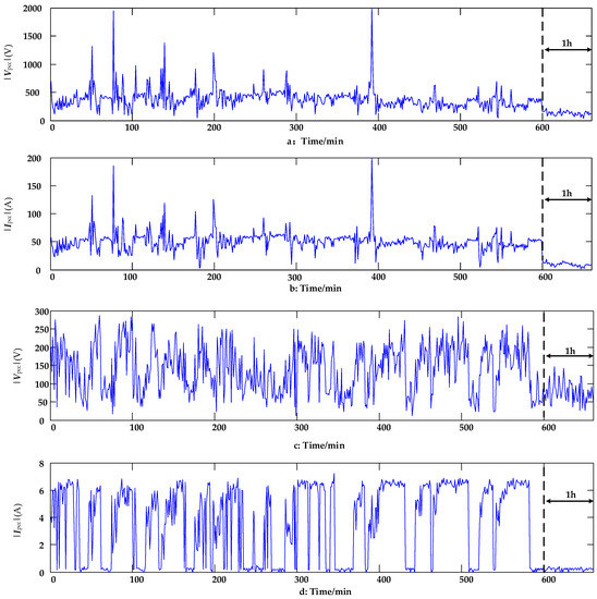
Figure 8.
Waveforms harmonic current and voltage amplitude at PCC: (a) Magnitude of 3rd harmonic voltage; (b) magnitude of 3rd harmonic current; (c) magnitude of 11th harmonic voltage; (d) magnitude of 11th harmonic current.
According to the field data shown in Figure 8, the utility 3rd and 11th harmonic impedances are calculated using Method 1 and the proposed method. The calculation results of the magnitude and the angle of the utility harmonic impedance are shown in Figure 9.
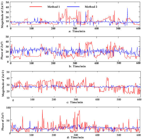
Figure 9.
The magnitude and phase of utility harmonic impedance: (a) Magnitude of 3rd harmonic impedance; (b) phase of 3rd harmonic impedance; (c) magnitude of 11th harmonic impedance; (d) phase of 11th harmonic impedance.
During the stable operation period of the power system, the operation mode does not change in most cases, and the fluctuation in the impedance of the utility side is small, which means that the magnitude and angle of the impedance are nearly constant. As can be seen from Figure 9, the calculation results of the two methods fluctuated. Moreover, even though there is some fluctuation in the results of the two methods, the fluctuation of calculation results obtained by utilizing the proposed method is smaller than with Method 1. This is because there are only 60 sample points involved in each computation, which is insufficient for the classical ICA algorithm. For the classical ICA algorithm, a reliable and stable result can be obtained only when there are lots of sample data involved in the computation; therefore, the calculation results of Method 1 show a large fluctuation. The proposed method can avoid the local optimum by adding the prior information of the utility side, which can reduce the amount of recorded data involved in each calculation. From Figure 9, it is clear that the calculation results of the proposed method are more stable than those of Method 1.
5. Conclusions
(1) Utility harmonic impedance is an important parameter for harmonic contribution estimation and harmonic mitigation. In this paper, a utility harmonic impedance estimation method based on the constrained independent component analysis is proposed to solve the problems in the classical ICA method by adding the prior information of the utility harmonic source into the objective function of the ICA algorithm. Compared with the classical method, the proposed method can obtain the global optimum and reduce the iteration times; therefore, the performance of the proposed method is better than that of the classical method. The performance of the proposed method is verified by simulations and field testing.
(2) The computer simulation and field test results showed that the proposed method is more robust to the fluctuation of background harmonic compared with the method based on ComplexICA. Also, the estimation error is smaller than with the classical ICA method and a more stable estimation result can be obtained even when there are fewer recorded data. Therefore, the proposed method is more effective when real-time impedance data are needed and can reduce the amount of the calculation because of fewer recorded data, so the proposed method is more suitable for engineering applications.
(3) Prior information of the utility side is a critical parameter in the proposed method. In this paper, the data recorded when the loads are shut down are chosen as the prior information. In order to extend the use of the proposed method, more suitable prior information of the utility side harmonic source should be selected. With more and more distributed generation and energy storage devices connected into the power system, a more effective utility harmonic impedance estimation method should be proposed in further research.
Author Contributions
X.X. proposed the original idea; X.Z. carried out the main research tasks and wrote the full manuscript; Y.W. double-checked the results and the whole manuscript; S.X. supported the writing and summarizing of the proposed ideas; Z.Z. contributed to the English translation.
Funding
This work was supported by the project “Economic Loss and Energy Efficiency of Power Quality Evaluation [SGRI-DL-71-15-006]” by the State Grid Corporation of China.
Conflicts of Interest
The authors declare no conflict of interest.
Abbreviations
| PCC | the point of common coupling |
| ICA | independent component analysis |
| ComplexICA | complex independent component analysis |
| CICA | constrained independent component analysis |
| ComplexCICA | complex constrained independent component analysis |
| FFT | fast Fourier transform |
| Lap (a, b) | Laplace distribution random variable with the expectation a and variance b |
References
- IEEE Recommended Practice and Requirements for Harmonic Control in Electric Power Systems; IEEE Std 519–2014; IEEE: New York, NY, USA, 2014.
- Electromagnetic Compatibility (EMC)—Part 3–6: Limits—Assessment of Emission Limits for the Connection of Distorting Installations to MV, HV and EHV Power Systems; IEC 61000-3-6; International Electrotechnical Commission (IEC): Geneva, Switzerland, 2008.
- Dolara, A.; Leva, S. Power Quality and Harmonic Analysis of End User Devices. Energies 2012, 5, 5453–5466. [Google Scholar] [CrossRef]
- Zang, T.L.; He, Z.Y.; Wang, Y. A Piecewise Bound Constrained Optimization for Harmonic Responsibilities Assessment under Utility Harmonic Impedance Changes. Energies 2017, 10, 936. [Google Scholar] [CrossRef]
- Girgis, A.A.; Mcmanis, R.B. Frequency domain techniques for modeling distribution or transmission networks using capacitor switching induced transients. IEEE Trans. Power Deliv. 1989, 4, 1882–1890. [Google Scholar] [CrossRef]
- Nagpal, M.; Xu, W.; Sawada, J. Harmonic impedance measurement using three-phase transients. IEEE Trans. Power Deliv. 1998, 13, 272–277. [Google Scholar] [CrossRef]
- Gretsch, R.; Neubauer, M. System impedances and background noise in the frequency range 2 kHz to 9 kHz. Eur. Trans. Electr. Power 1998, 8, 369–374. [Google Scholar] [CrossRef]
- Sumner, M.; Palethorpe, B.; Thomas, D.W.P. A technique for power supply harmonic impedance estimation using a controlled voltage disturbance. IEEE Trans. Power Electron. 2002, 17, 207–215. [Google Scholar] [CrossRef]
- Xu, W.; Ahmed, E.E.; Zhang, X. Measurement of network harmonic impedances: Practical implementation issues and their solutions. IEEE Trans. Power Deliv. 2002, 17, 210–216. [Google Scholar]
- Sumner, M.; Palethorpe, B.; Thomas, D.W.P. Impedance measurement for improved power quality—Part 1: The measurement technique. IEEE Trans. Power Deliv. 2004, 19, 1442–1448. [Google Scholar] [CrossRef]
- Yang, H.G.; Pirotte, P.; Robert, A. Harmonic emission levels of industrial loads statistical assessment. CIGRE 1996, 96, 1936–1996. [Google Scholar]
- Huang, X.; Nie, P.; Gong, H. A new assessment method of customer harmonic emission level. In Proceedings of the Asia-Pacific Power and Energy Engineering Conference (APPEEC 2010), Chengdu, China, 28–31 March 2010; pp. 1–5. [Google Scholar]
- Xiao, X.Y.; Yang, H.G. The method of estimating customers harmonic emission level based on bilinear regression. In Proceedings of the IEEE International Conference on Electric Utility Deregulation, Restructuring and Power Technologies, Hong Kong, China, 5–8 April 2004; pp. 662–665. [Google Scholar]
- Langella, R.; Testa, A. A New Method for Statistical Assessment of the System Harmonic Impedance and of the Background Voltage Distortion. In Proceedings of the International Conference on Probabilistic Methods Applied to Power Systems, Stockholm, Sweden, 11–15 June 2006; pp. 1–7. [Google Scholar]
- Mazin, H.E.; Xu, W.; Huang, B. Determining the Harmonic Impacts of Multiple Harmonic—Producing Loads. IEEE Trans. Power Deliv. 2011, 26, 1187–1195. [Google Scholar] [CrossRef]
- Hui, J.; Yang, H.G. Assessing utility harmonic impedance based on the covariance characteristic of random vectors. IEEE Trans. Power Deliv. 2010, 25, 1778–1786. [Google Scholar] [CrossRef]
- Hui, J.; Freitas, W.; Vieira, J.C.M. Utility harmonic impedance measurement based on data selection. IEEE Trans. Power Deliv. 2012, 27, 2193–2202. [Google Scholar] [CrossRef]
- Tang, B.; Ma, S.; Lin, S.F.; Chen, G.; Fu, Y. Harmonic current emission level assessment of residential loads based on impedance-gathering trend. Int. Trans. Electr. Energy Syst. 2017, 27, e2337. [Google Scholar] [CrossRef]
- Borkowski, D. A new method for noninvasive measurement of grid harmonic impedance with data selection. Int. Trans. Electr. Energy Syst. 2015, 25, 3772–3791. [Google Scholar] [CrossRef]
- Borkowski, D.; Wetula, A.; Bień, A. New method for noninvasive measurement of utility harmonic impedance. In Proceedings of the Power and Energy Society General Meeting, San Diego, CA, USA, 22–26 July 2012; pp. 1–8. [Google Scholar]
- Zhao, X.; Yang, H.G. A New Method to Calculate the Utility Harmonic Impedance Based on FastICA. IEEE Trans. Power Deliv. 2016, 31, 381–388. [Google Scholar] [CrossRef]
- Karimzadeh, F.; Esmaeili, S.; Hossein, H.S. Method for determining utility and consumer harmonic contributions based on complex independent component analysis. IET Gener. Transm. Distrib. 2016, 10, 526–534. [Google Scholar] [CrossRef]
- Liao, H.W.; Niebur, D. Load profile estimation in electric transmission networks using independent component analysis. IEEE Trans. Power Syst. 2003, 18, 707–715. [Google Scholar] [CrossRef]
- Yu, X.C.; Hu, D. Independent component analysis. In Book Blind Source Separation Theory and Application, 1st ed.; Zhang, Y.F., Ed.; Science Press: Beijing, China, 2011; pp. 65–67. [Google Scholar]
- Berckmoes, B.; Molenberghs, G. Approximate Central Limit Theorems. J. Theor. Probab. 2018, 31, 1–16. [Google Scholar] [CrossRef]
- Wei, L.; Rajapakse, J.C. Constrained Independent Component Analysis. Adv. Neural Inf. Process. Syst. 2001, 13, 570–576. [Google Scholar]
- Wang, P.; Goel, L.; Liu, X. Harmonizing AC and DC: A Hybrid AC/DC Future Grid Solution. IEEE Power Energy Mag. 2013, 11, 76–83. [Google Scholar] [CrossRef]
- Hosseinzadeh, M.; Salmasi, F.R. Robust Optimal Power Management System for a Hybrid AC/DC Micro–Grid. IEEE Trans. Sustain. Energy 2015, 6, 675–687. [Google Scholar] [CrossRef]


© 2018 by the authors. Licensee MDPI, Basel, Switzerland. This article is an open access article distributed under the terms and conditions of the Creative Commons Attribution (CC BY) license (http://creativecommons.org/licenses/by/4.0/).