A New Transient Frequency Acceptability Margin Based on the Frequency Trajectory

Abstract

When the electric power system is disturbed, the transient frequency deviation may be large and harmful to its stable operation, especially in some small power systems. However, there is a lack of transient frequency acceptability margin (TFAM) which could be directly used by dispatchers. In this paper, a new TFAM is proposed based on the transient frequency acceptability index (TFAI). First, based on the frequency trajectory and the philosophy of “different weights to the different frequency offset levels”, a new TFAI is proposed combined with frequency thresholds and time duration limits. The effectiveness of the TFAI is verified, and the critical acceptable disturbance is determined by using the TFAI. Then, a new TFAM is proposed based on the critical acceptability disturbance. The proposed TFAM can quantitatively describe the distance of the operation point from the critical frequency acceptability point, and distinguish the transient frequency acceptability of different disturbances. Finally, with different simulations, the effectiveness and applicability of the proposed TFAM are verified. The TFAM can be used for disturbances with single-parameter and multiple parameters.

1. Introduction

Frequency reflects the active power balance of generator output and load in the power system. Frequency deviation that is overly large will lead to serious consequences for the safe operation of generators and systems as well as users. For example, equipment such as generators and auxiliary machines will deviate from working conditions, thus reducing their efficiency, affecting the economic operation of power plants and also of the entire power grid. If the frequency is too low, it will also endanger the safe operation of the whole system. Therefore, it is necessary to evaluate the transient frequency characteristics of a power system under different disturbances to determine whether the frequency can remain stable [1,2,3,4]. At present, more and more photovoltaic and wind power sources are being connected to power systems, which brings more frequency instability problems. Research by [5,6] relates to this problem.

Compared with large-scale power grids, frequency instability has a greater impact on distributed systems. For frequency stability evaluation and control of distributed systems, scholars have conducted significant research. Ref. [7] modeled inverter-based distributed generators to research the stability of a microgrid. Ref. [8] suggested that the impacts of different penetration levels and distributed generation (DG) technologies on frequency stability are different. To determine frequency stability, Ref. [9] compared two stability indexes used for load shedding of the islanded distribution network and proposed an under-frequency load shedding (UFLS) algorithm. Similarly, Ref. [10] proposed a novel load shedding strategy by considering power stability with economy in load shedding for a distribution system with distributed generation. Ref. [11] introduced a hierarchical frequency control strategy to ensure the power balance and frequency stability in multiple time scales for medium-voltage (MV) isolated microgrids.

In addition to distributed systems, transient frequency problems of large-scale power systems have also been studied. In general, the work in the assessment for the transient frequency characteristics can be divided into two categories. One is transient frequency stability assessment [2,3,4,5,6,7,8,9,10], which determines the stability of the transient frequency. The other is frequency acceptability assessment [11,12,13,14,15,16,17,18], which assesses whether the duration of frequency offset exceeding a specified value exceeds the regulation requirements after the power system suffers disturbances.

In the aspect of transient frequency stability, the traditional time domain simulation method [3,4] is more accurate, but takes longer and requires a large amount of computation, which is not conducive to rapid application.

With the advent of phasor measurement unit (PMU) and wide area measurement system (WAMS) [12,13,14], scholars have put forward online quantitative evaluation methods of steady-state frequency stability based on PMU data [15,16,17]. Ref. [15] estimated the system active vacancy by using the pre-disturbance PMU data to realize the steady-state frequency prediction. Based on Ref. [15], according to the PMU information, Ref. [16] considers the variation of load and transmission loss between the instantaneous after disturbance and the steady-state after disturbance. Ref. [17] used PMU data to predict the steady frequency and then determine the stability. It is worth noting that the above frequency stability determination methods ignore the transient process and cannot describe the impact of the transient process. Ref. [18] proposed a new approach to dynamic stability assessment of a power system. This approach applied the supervised concept to a clustering neural network, and directly used the frequencies of buses. Based on a complete-linkage clustering, Ref. [19] presented a methodology for selecting a set of critical operating points suitable for frequency stability assessments. In order to analyze the impact of rapid changes in the measurements on instability detection, a frequency trend vector is considered in Refs. [20,21] calculates interference power by using the real-time initial rate of change of frequency (ROCOF) from the WAMS, and then compares this power with the power mismatch threshold derived from the low-order system frequency response (SFR) model to judge the severity of the interference. Similarly, [22] used the ROCOF and maximum frequency deviation to determine the frequency stability.

To describe the impact of the transient process in transient frequency acceptability assessment, Ref. [23] proposed to use a fixed frequency drop threshold and time duration when frequency is abnormal to form a number of two-element tables to quantitatively assess the acceptability of transient frequency offset. On this basis, three transient frequency offset margin indices were proposed by [24,25,26], and the quantitative analysis of security of transient frequency offset was realized. The two indices of [24,25] can be applied to the optimization of under-frequency load shedding (UFLS). Ref. [27] proposed that these margins should be based on the center of inertia frequency. Further, Ref. [28] considered the influence of frequency offset and proposed a transient frequency acceptability index based on the cumulative effect. On this basis, Ref. [29] proposed a frequency margin index which can evaluate the severity of faults.

In recognizing that the above proposed indices take the same weights for different frequency drops and cannot distinguish the influence of different drop degrees, Ref. [30] proposed a transient frequency acceptability evaluation index which uses different weighting factors for different drop degrees, and applied it to the transient frequency acceptability evaluation and security control of a power grid connected by large-scale thermal power units. Further, Ref. [31] expanded this index to the frequency acceptability assessment of a large-scale power grid with wind farms. Ref. [32] improved the index to analyze the transient frequency acceptability when the frequency drops.

It is worth noting that the index proposed by [30,31,32] is difficult to be used to compare frequency deviation acceptability directly under different faults. Hence, this index is not suitable for a dispatcher to directly judge frequency deviation acceptability.

In recognizing the above problems, based on [30,32], this paper proposes an improved transient frequency acceptability index (TFAI) and, furthermore, proposes a new transient frequency acceptability margin (TFAM) referring to the philosophy of security domain [33,34]. This margin can determine the distance between the current running point of the system and the frequency collapse point, so as to analyze the degree of transient frequency deviation and make it convenient for the dispatcher to determine the degree of transient frequency deviation acceptability. The main contributions of this paper are as follows:

(1)

The TFAI proposed in this paper can use frequency deviation information to quantitatively evaluate frequency acceptability.

(2)

By comparing real-time parameters and the parameters obtained by off-line simulation, the TFAM proposed in this paper directly provides the distance between the current operating point and the critical boundary. This facilitates the dispatcher to judge the frequency acceptability and take measures.

(3)

The TFAM proposed in this paper is expressed in power space and considers the power mismatch. Compared with other frequency margins, the TFAM is more convenient to formulate security control measures.

(4)

The TFAM proposed in this paper can be used to compare the transient frequency deviation acceptability under different faults.

The organization of the remainder of this paper is as follows. Section 2 introduces the construction of TFAI and TFAM. In Section 3, the relevant parameters of TFAI are determined according to the specific situation of small power grid Z, and the validity of TFAI is verified. Section 4 verifies the effectiveness of TFAM in many cases, focusing on the power grid Z. Finally, Section 5 draws conclusions and provides discussion.

2. The Construction of the TFAM

This section first presents a new transient frequency acceptability index (TFAI) and, then, proposes a new transient frequency acceptability margin (TFAM).

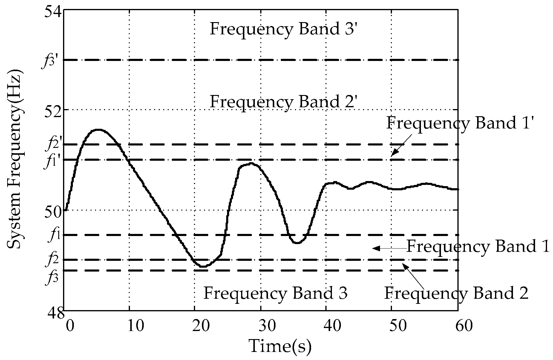
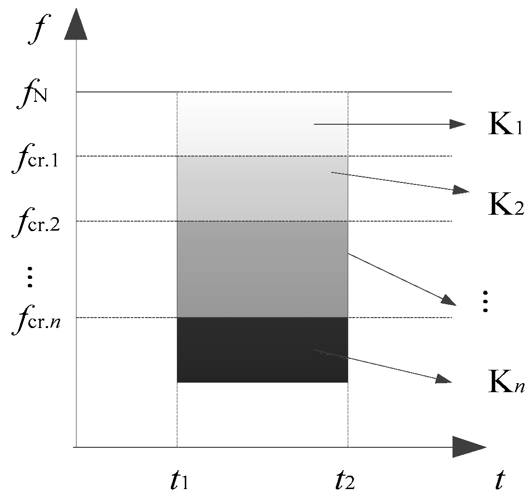
2.1. Transient Frequency Acceptability Index

The philosophy of the TFAI lies in assigning different weights to the accumulation of frequency deviation; that is, as shown in Figure 1, by dividing the frequency deviation into different bands (f₁-f₂, f₂-f₃, lower than f₃ and f_1′-f_2′, f_2′-f_3′, higher than f_3′), and applying different weights while integrating the frequency in the different bands.

Mathematically, the TFAI F can be expressed as follows:

$$F={\displaystyle \sum _{i=0}^n[{\displaystyle \sum _{j=1}^m{\mathrm{K}}_j}}{g}_j(f[t_i])\left|f[t_i]-f_{\mathrm{N}}\right|\mathsf{\Delta }{t}_i+{\displaystyle \sum _{k=1}^p{\mathrm{H}}_k{h}_k(f[t_i])\left|f[t_i]-f_{\mathrm{N}}\right|\mathsf{\Delta }{t}_i}]$$

(1)

where

$$g_j(f[t_i])=\{\begin{array}{c}\begin{array}{cc}1& \left(f_{j+1}\le f[t_i]\le f_j\right)\end{array}\\ \begin{array}{cc}0& \left(f[t_i]<f_{j+1}\mathrm{or}f[t_i]>f_j\right)\end{array}\end{array}$$

$$h_k(f[t_i])=\{\begin{array}{c}\begin{array}{cc}1& \left(f_k^{\prime }\le f[t_i]\le f_{k+1}^{\prime }\right)\end{array}\\ \begin{array}{cc}0& \left(f[t_i]<f_k^{\prime }\mathrm{or}f[t_i]>f_{k+1}^{\prime }\right)\end{array}\end{array}$$

and f[t_i] is the frequency at time t_i on the frequency trajectory; f_N is the rated frequency; f_k’ is the lower frequency of the frequency band k’ that is higher than the rated frequency; f_j is the upper frequency of the frequency band j that is below the rated frequency; Δt_i is the time step of the frequency response calculation; K_j is the weight factor of different frequency band j that is below the rated frequency; H_k is the weight factor of different frequency band k’ that is higher than the rated frequency; n is the number of sampling points; m is the number of frequency bands that are below the rated frequency; p is the number of frequency bands that are higher than the rated frequency.

The TFAI (Equation (1)) reflects frequency acceptability under a certain disturbance. At the same time, the weight factors of the TFAI can be adjusted according to the requirements of the frequency acceptability.

The presented TFAI first judges whether the frequency enters a certain frequency band, and then assigns different weights to the frequency in its vertical direction (fall depth or rising height). Thus, the TFAI can reflect the influence of different frequency offsets and improve the accuracy of the frequency acceptability evaluation.

Compared to [30,31], the improvement of this paper is that for a certain sampling point, the proposed TFAI first judges the frequency band of the sampling point. Then, the TFAI only considers the weight of this frequency band, and avoids the interference of weights of other frequency bands. For example, as shown in Figure 2, the proposed TFAI is K_n × (f_N − f), while in [30,31], the acceptability index is K_n × (f_N − f) + K_n−1 × (f_N − f_cr.n−1) +⋯ + K₂ × (f_N − f_cr.2) + K₁ × (f_N − f_cr.1). This index is influenced by weights of other bands, such as K_n−1, …, K₂, K₁.

In addition, compared with [32], the proposed TFAI can analyze the frequency acceptability when the frequency rises and falls.

2.2. Transient Frequency Acceptability Margin

This section proposes a transient frequency acceptability margin from the viewpoint of the dispatchers/operators based on the TFAI presented in Section 2.1.

As shown in Section 2.1, the TFAI can evaluate the acceptability of the transient frequency. However, the degree of frequency acceptability cannot be displayed directly in the power space, and the distance between the current operating point of the system and the acceptable margin is implicitly contained. Therefore, it is necessary to construct a transient frequency acceptability margin in the power space, i.e., from the viewpoint of the dispatchers/operators.

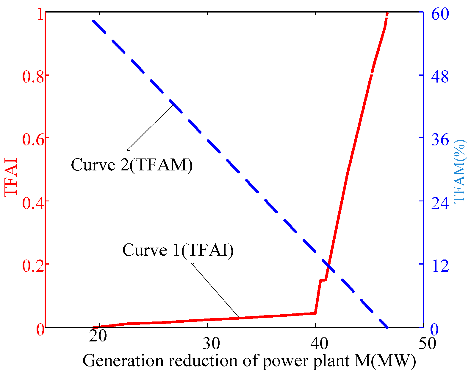
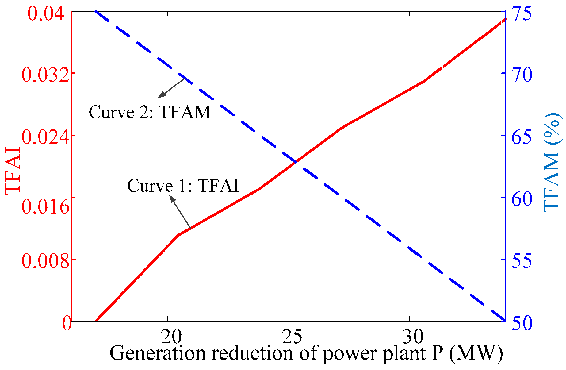
2.2.1. Power Disturbance with Single Parameter

For a specific active disturbance with parameter ΔP_dist, the TFAI F(ΔP_dist) can be obtained. If there is a value ΔP_dist = ΔP_cr, which satisfies F(ΔP_cr) = 1, then the disturbance ΔP_cr is the disturbance which may lead to transient frequency critical unacceptability under such disturbance.

The relationship between ΔP_cr and the actual disturbance ΔP_dist can reflect the frequency acceptability under the disturbance, that is, if ΔP_cr > ΔP_dist, then the transient frequency is acceptable; otherwise, the transient frequency is not acceptable. Therefore, the TFAM can be described by the difference between ΔP_cr and ΔP_dist, i.e.,

$${\eta }^{\prime }=\mathsf{\Delta }{P}_{\mathrm{cr}}-\mathsf{\Delta }{P}_{\mathrm{dist}}$$

(2)

In order to compare the frequency acceptability of different disturbances, the normalized TFAM under disturbance i could be defined as follows:

$${\eta }_i=\frac{\mathsf{\Delta }{P}_{\mathrm{cr}i}-\mathsf{\Delta }{P}_{\mathrm{dist}i}}{\mathsf{\Delta }{P}_{\mathrm{cr}i}}\times 100\%$$

(3)

where ΔP_disti is the parameter under the disturbance i; ΔP_cri is the critical value corresponding to the transient frequency acceptability of system under the disturbance i.

With normalization, the TFAM of the disturbance i decreases linearly with the increase of the value of the parameter of the actual disturbance. If there is no disturbance, then ΔP_disti = 0, and the margin is 100%. If ΔP_disti = ΔP_cri, the transient frequency is critical acceptable and the margin is 0.

In particular, under a single fault, when ΔP_cri is greater than the maximum disturbance quantity ΔP_max, e.g., the maximum generator tripping quantity and load shedding quantity, it is impossible to obtain ΔP_cri by simulation. In this case, with experience, the critical value could be set as ΔP_cri = 2ΔP_max for the sake of unified consideration.

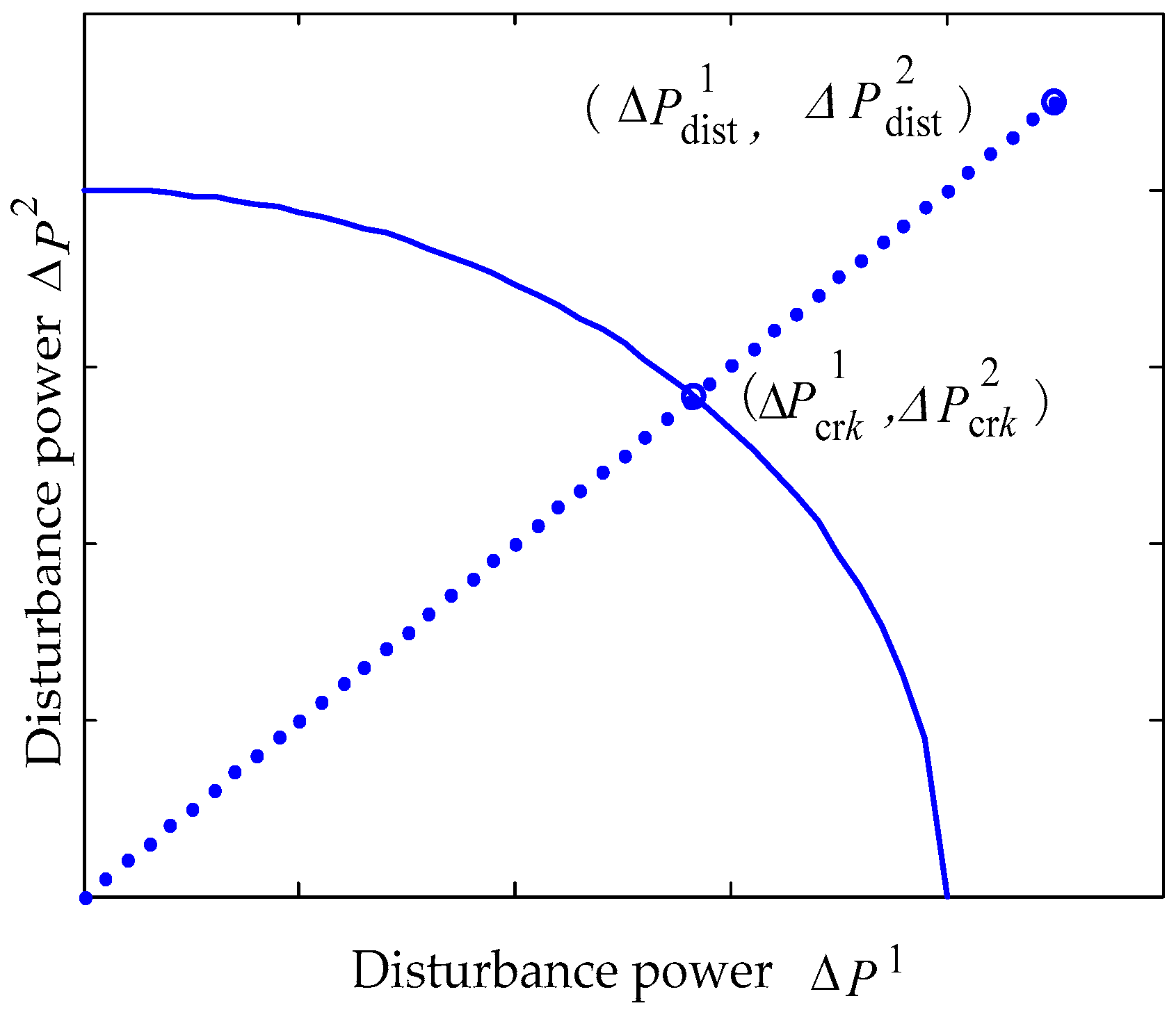
2.2.2. Power Disturbance with Multiple Parameters

When a disturbance involves changes of multiple parameters, the multiple n parameters can form an n-dimensional vector (ΔP_dist¹, ΔP_dist², …, ΔP_distⁿ).

The normalized distance of the current disturbance point from any critical point k (ΔP_crk¹, ΔP_crk², …, ΔP_crkⁿ) on the critical acceptability boundary can be defined as:

$${\epsilon }^{(k)}=\frac{\sqrt{{\displaystyle \sum _{i=1}^n{\left(\mathsf{\Delta }{P}_{\mathrm{cr}k}^i-\mathsf{\Delta }{P}_{\mathrm{dist}}^i\right)}^2}}}{\sqrt{{\displaystyle \sum _{i=1}^n{(\mathsf{\Delta }{P}_{\mathrm{cr}k}^i)}^2}}}$$

(4)

If the transient frequency under the disturbance is unacceptable, then the TFAM under the disturbance can be defined as:

$$\eta =\underset{k}{-\min }\left|{\epsilon }^{(k)}\right|$$

(5)

If the transient frequency under the disturbance is acceptable, the TFAM under the disturbance can be defined as:

$$\eta =\underset{k}{\min }{\epsilon }^{(k)}$$

(6)

In the case of n = 2, the parameter of the disturbance is two-dimensional, i.e., (ΔP_dist¹, ΔP_dist²). This vector and the critical point k (ΔP_crk¹, ΔP_crk²) on the critical acceptability boundary are shown in Figure 3.

Equation (4) can then be expressed as:

$${\epsilon }^{(k)}=\frac{\sqrt{{\left(\mathsf{\Delta }{P}_{\mathrm{cr}k}^1-\mathsf{\Delta }{P}_{\mathrm{dist}}^1\right)}^2+{\left(\mathsf{\Delta }{P}_{\mathrm{cr}k}^2-\mathsf{\Delta }{P}_{\mathrm{dist}}^2\right)}^2}}{\sqrt{{(\mathsf{\Delta }{P}_{\mathrm{cr}k}^1)}^2+{(\mathsf{\Delta }{P}_{\mathrm{cr}k}^2)}^2}}$$

(7)

2.2.3. Increase of the Disturbance Parameters in the Fixed Direction

If the disturbance parameters increase in the fixed direction (assuming n parameters), the direction of the disturbance is fixed. Assuming the direction is λ ∈ Rⁿ and ‖λ‖= 1, the critical frequency acceptability point in this direction could be described as follows:

$$(\mathsf{\Delta }{P}_{\mathrm{cr}k}^1,\mathsf{\Delta }{P}_{\mathrm{cr}k}^2,\dots ,\mathsf{\Delta }{P}_{\mathrm{cr}k}^n)=l_{\mathrm{cr}}\cdot \lambda$$

(8)

where l_cr is a real number equal to $\sqrt{{\sum }_{i=1}^n{\left(\mathsf{\Delta }{P}_{\mathrm{cr}k}^i\right)}^2}$ in Equation (4).

Because the direction of the disturbance is fixed, any disturbance point can be described as follows:

$$(\mathsf{\Delta }{P}_{\mathrm{dist}}^1,\mathsf{\Delta }{P}_{\mathrm{dist}}^2,\dots ,\mathsf{\Delta }{P}_{\mathrm{dist}}^n)=l\cdot \lambda$$

(9)

where l is a real number.

Here, the TFAM can be defined as:

$$\eta =\frac{l_{\mathrm{cr}}-l}{l_{\mathrm{cr}}}$$

(10)

where l_cr − l equals $\sqrt{{\sum }_{i=1}^n{\left(\mathsf{\Delta }{P}_{\mathrm{cr}k}^i-\mathsf{\Delta }{P}_{\mathrm{dist}}^i\right)}^2}$ in Equation (4).

In particular, when n = 2, λ ∈ R², l_cr equals $\sqrt{{\left(\mathsf{\Delta }{P}_{\mathrm{cr}k}^1\right)}^2+{\left(\mathsf{\Delta }{P}_{\mathrm{cr}k}^2\right)}^2}$ in Equation (7), and l_cr − l equals $\sqrt{{\left(\mathsf{\Delta }{P}_{\mathrm{cr}k}^1-\mathsf{\Delta }{P}_{\mathrm{dist}}^1\right)}^2+{\left(\mathsf{\Delta }{P}_{\mathrm{cr}k}^2-\mathsf{\Delta }{P}_{\mathrm{dist}}^2\right)}^2}$ in Equation (7).

When the disturbance power point is on the unacceptable side of the critical acceptability boundary, l > l_cr, and η < 0. The greater is l, the smaller is η, and the further the disturbance power point from the critical stability point. Here, it can be judged by the TFAM η that the degree of frequency unacceptability increases gradually.

When the disturbance power point is on the acceptable side of the critical acceptability boundary, l < l_cr, and η > 0. The greater is l, the smaller is η, and the closer the disturbance power point to the critical stability point. Here, it can be judged by the TFAM η that the degree of frequency acceptability decreases gradually.

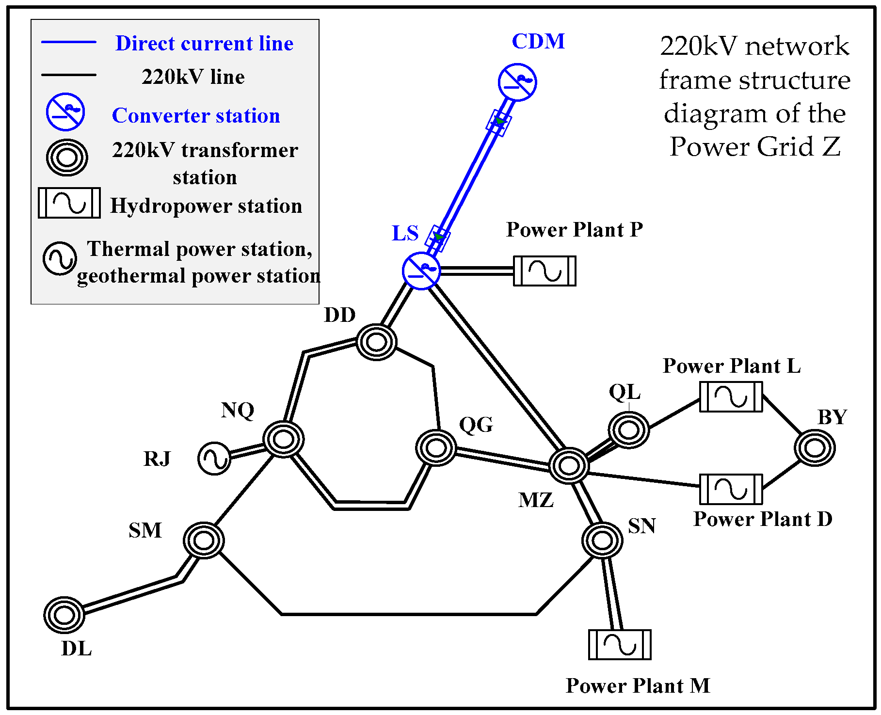
3. TFAI for the Small Power Grid Z

This section derives the TFAI for the small power grid Z, as shown in Figure 4, which is modeled in the software PSD-BPA. The total load of Z is about 700 MW. The hydraulic power plant M has the largest proportion among all the power plants, i.e., 195 MW (three generators with 65 MW), which is 28.1% of the load. The measurement of the frequency is located at power plant M.

3.1. Frequency Bands and Time Duration Limits

For the small power grid Z, the normal frequency fluctuation range (or acceptable frequency range) is 50 ± 0.5 Hz, so there is no weight factor in the 50 ± 0.5 Hz band (i.e., the weight is 0).

The setting of the under frequency load shedding (UFLS) is: first round operation frequency is 48.8 Hz, and delay time is 0.3 s; the special round operation frequency is 49.0 Hz, and the delay time is 10 s. Furthermore, the action of UFLS should be avoided as far as possible to maintain frequency acceptability. Thus, the first acceptable frequency sag is that the duration when the frequency is below 48.8 Hz does not exceed 0.3 s. The second acceptable frequency sag is that the duration when the frequency is below 49.0 Hz does not exceed 10 s.

Moreover, Chinese standard “DLT 1234-2013 Technique specification of power system security and stability calculation” [35] demands that the frequency should recover to more than 49.5 Hz after the UFLS devices operate. Consequently, the time duration when the transient frequency is below 49.5 Hz should not exceed 10 min.

Therefore, for the low frequency section in Figure 1, according to the system safety requirements, the frequency trajectory can be divided into three bands. From low to high, the three bands are below 48.8 Hz, 48.8–49.0 Hz, and 49.0–49.5 Hz, and the corresponding weight factors are K₃, K₂, and K₁, respectively.

In the high frequency case, the first round operation frequency of the high frequency generator tripping of the small power grid Z is 53 Hz, and the delay time is 0.3 s. To avoid the interference of high frequency generator tripping on frequency acceptability, the time duration when the frequency is beyond 53 Hz should not exceed 0.3 s. Moreover, the operation frequency of over-speed protection control (OPC) of the power grid Z is 51.3 Hz, and the delay time is 10 s. This requires that the time duration when the transient frequency is higher than 51.3 Hz should not exceed 10 s. Chinese standard “DLT 1234-2013 Technique specification of power system security and stability calculation” [35] demands that the frequency cannot be more than 51 Hz for a long period. Consequently, the time duration when the frequency is beyond 51 Hz should not exceed 180 s.

Therefore, for the high frequency section in Figure 1, the frequency trajectory can be divided into three bands. From high to low, the three bands are above 53 Hz, 51.3–53 Hz and 51–51.3 Hz, and the corresponding weight factors are H₃, H₂, and H₁, respectively.

3.2. Determination of Weight Factors

The setting of the weight factors makes the result of the TFAI F more than or equal to 1 when the requirements are not satisfied. Thus, the weight factors K₁, K₂, and K₃ for the low frequency section, corresponding to different frequency bands, should satisfy the following equations:

$$\{\begin{array}{c}F={\mathrm{K}}_3\times \left(50-48.8\right)\times 0.3=1\\ F={\mathrm{K}}_2\times \left(50-49.0\right)\times 10=1\\ F={\mathrm{K}}_1\times \left(50-49.5\right)\times 600=1\end{array}$$

(11)

where the first equation in Equation (11) means that if the time duration when the frequency is lower than 48.8 Hz exceeds 0.3 s, the TFAI F = 1. The equation corresponds to the requirement of avoiding action of the first round of UFLS. Similarly, the second equation means that if the time duration when the frequency is lower than 49.0 Hz exceeds 10 s, F = 1. The equation corresponds to the requirement of avoiding action of the special round of UFLS. The third equation means that if the time duration when the frequency is lower than 49.5 Hz exceeds 600 s, F = 1. The equation corresponds to the requirement of frequency acceptability. The threshold-delay parameters and weight factors for the low frequency band can be summarized as shown in

Table 1. Low frequency threshold-delay parameters and weight factors.

Threshold-delay parameter	(49.5, 600)	(49, 10)	(48.8, 0.3)
Weight factor	K1	K2	K3
Value of weight factor	0.0033	0.1000	2.7778

.

For the high frequency section, the weight factors H₁, H₂, and H₃ should satisfy the following equations:

$$\{\begin{array}{c}F={\mathrm{H}}_3\times (53-50)\times 0.3=1\\ F={\mathrm{H}}_2\times (51.3-50)\times 10=1\\ F={\mathrm{H}}_1\times (51-50)\times 180=1\end{array}$$

(12)

where the first equation in Equation (12) means that if the time duration when the frequency is higher than 53 Hz exceeds 0.3 s, the TFAI F = 1. The second equation means that if the time duration when the frequency is higher than 51.3 Hz exceeds 10 s, F = 1. The third equation means that if the time duration when the frequency is higher than 51 Hz exceeds 180 s, F = 1. The threshold-delay parameters and weight factors for the high frequency bands can be summarized as shown in

Table 2. High frequency threshold-delay parameters and weight factors.

Threshold-delay parameter	(51, 180)	(51. 3,10)	(53, 0.3)
Weight factor	H1	H2	H3
Value of weight factor	0.0056	0.0769	1.1111

.

In general, the TFAI including the high and the low frequency sections can be expressed as follows.

$$\begin{array}{ll}F=& {\displaystyle \sum _{i=0}^n[0.0033\times g_1(f[t_i])\left|f[t_i]-f_{\mathrm{N}}\right|\mathsf{\Delta }{t}_i}+0.1000\times g_2(f[t_i])\left|f[t_i]-f_{\mathrm{N}}\right|\mathsf{\Delta }{t}_i\\ & +2.7778\times g_3(f[t_i])\left|f[t_i]-f_{\mathrm{N}}\right|\mathsf{\Delta }{t}_i+0.0056\times h_1(f[t_i])\left|f[t_i]-f_{\mathrm{N}}\right|\mathsf{\Delta }{t}_i\\ & +0.0769\times h_2(f[t_i])\left|f[t_i]-f_{\mathrm{N}}\right|\mathsf{\Delta }{t}_i+1.1111\times h_3(f[t_i])\left|f[t_i]-f_{\mathrm{N}}\right|\mathsf{\Delta }{t}_i]\end{array}$$

(13)

where

$$g_j(f[t_i])=\{\begin{array}{c}\begin{array}{cc}1& \left(f_{j+1}\le f[t_i]\le f_j\right)\end{array}\\ \begin{array}{cc}0& \left(f[t_i]<f_{j+1}\mathrm{or}f[t_i]>f_j\right)\end{array}\end{array}$$

$$h_k(f[t_i])=\{\begin{array}{c}\begin{array}{cc}1& \left(f_k^{\prime }\le f[t_i]\le f_{k+1}^{\prime }\right)\end{array}\\ \begin{array}{cc}0& \left(f[t_i]>f_{k+1}^{\prime }\mathrm{or}f[t_i]<f_k^{\prime }\right)\end{array}\end{array}$$

and f[t_i] is the frequency at time t_i; f_N is the system rated frequency; f_k’ is the lower frequency of the frequency band k’ which is higher than the rated frequency; f_j is the upper frequency of the frequency band j which is below the rated frequency; Δt_i is the time step of the frequency response calculation.

When F ≥ 1, the frequency deviation is unacceptable, and measures need to be taken. When F < 1, the frequency deviation is acceptable.

In calculation of the proposed TFAI, only the weights of the frequency bands in which the sampling points are located are used, and the weights of other frequency bands are not included. In [30,31], the calculation required the weights of other frequency bands between the frequency sampling point and the rated frequency.

3.3. Determination of Sampling Interval

This subsection analyzes the impact of time interval on the result of TFAI and determines the suitable time interval.

If disturbance A is set as the load at bus ZD of the small power grid Z increasing 50 MW, then the frequency trajectory under disturbance A can be obtained as shown in Figure 5.

Figure 5 shows that the frequency satisfies the three requirements of frequency acceptability, thus the system is transient frequency acceptable under disturbance A. Furthermore, the TFAI with different sampling intervals can be obtained as shown in

Table 3. TFAI with different sampling intervals.

Sampling interval/s	0.02	0.04	0.1
TFAI	0.9616	6.0280	126.1728

.

As shown in Table 3, when the sampling interval is 0.02 s, the TFAI is less than 1, however, when the sampling interval is 0.04 s and 0.1 s, the TFAI is greater than 1, which is not consistent with the conclusion that the transient frequency under disturbance A is acceptable.

Clearly, with the increase of sampling interval, some useful information will be lost, and the result may have a larger error. The smaller the sampling interval, the closer the value to the true value (integration). Moreover, the time interval of PMU data could be set to 0.02 s, 0.04 s or 0.1 s. Therefore, in the application of the proposed index, the time interval of 0.02 s is recommended.

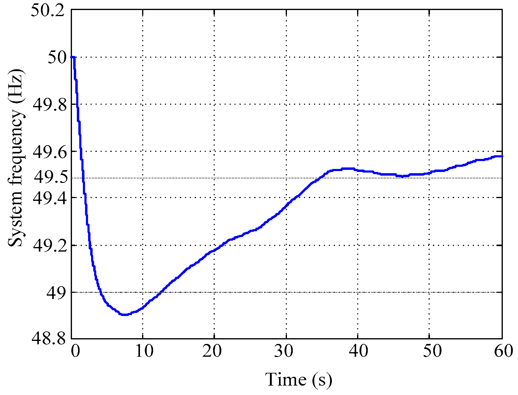
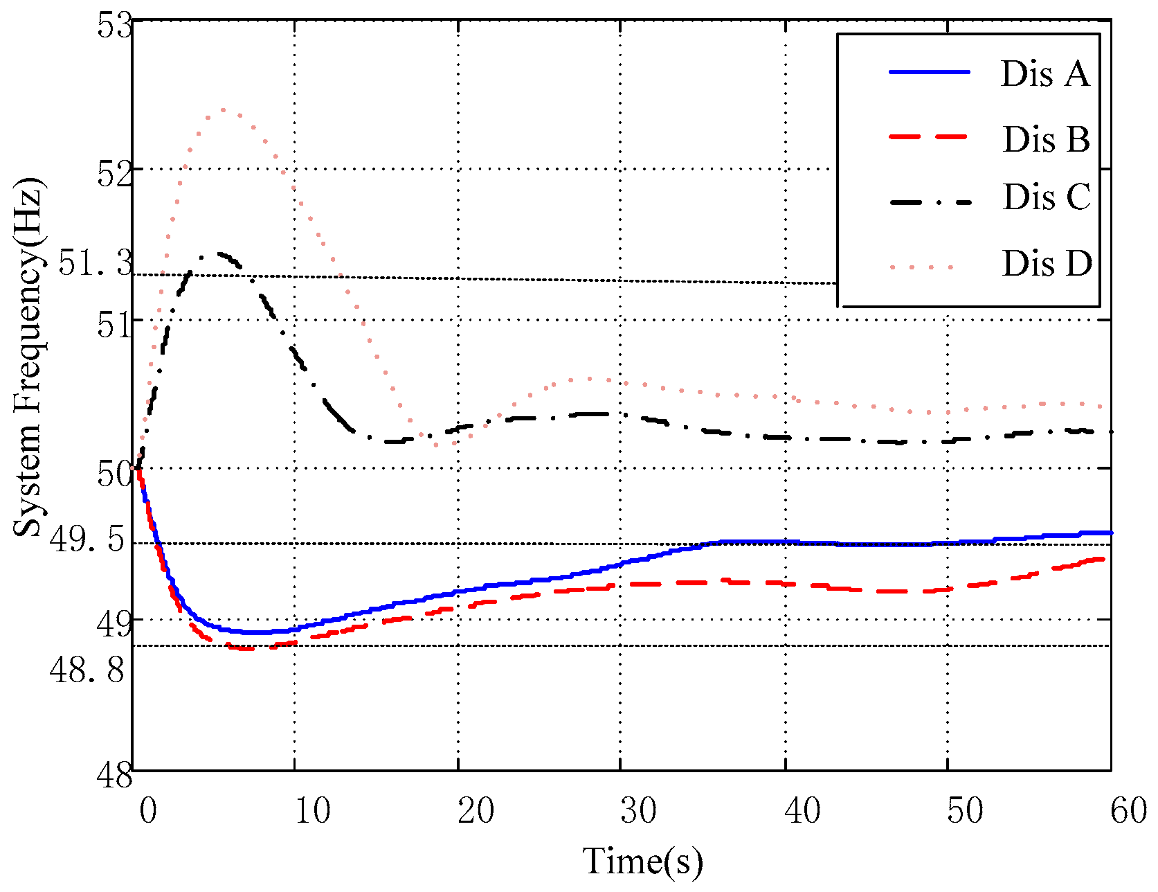
3.4. Effectiveness of the Proposed TFAI

This subsection verifies the effectiveness of the proposed TFAI with different disturbances.

The different disturbances are listed as follows.

(1)

Dis A: the load at bus ZD increases 50 MW.

(2)

Dis B: the load at bus ZD increases 55 MW.

(3)

Dis C: the load at bus H decreases 60 MW.

(4)

Dis D: the load at bus H decreases 130 MW, the load at bus DG decreases 15 MW.

The frequency trajectories under the above four disturbances are shown in Figure 6 and the corresponding TFAI and evaluation results are shown in

Table 4. The TFAI under four disturbances and transient frequency acceptability.

Disturbance	TFAI	Transient Frequency Acceptability
Dis A	0.9616	Acceptable
Dis B	1.5620	Unacceptable (The time duration of the frequency lower than 49 Hz is 13.01 s, more than 10 s)
Dis C	0.4025	Acceptable
Dis D	1.6752	Unacceptable (The time duration of the frequency higher than 51.3 Hz is 11.3 s, more than 10 s)

.

Figure 6 shows that the system is transient frequency acceptable under Dis A and C. Table 4 shows that TFAI for Dis A and C are 0.9616 and 0.4025 respectively, which are both less than 1 and indicate that the frequency deviation is acceptable.

Furthermore, Figure 6 shows that for Dis B, the time duration when the system frequency is below 49 Hz is 13.01 s, greater than the permissible time of 10 s, thus the frequency deviation is unacceptable. Table 4 shows that TFAI for Dis B is 1.5620, larger than 1, which indicates that the system frequency deviation is unacceptable.

The results for Dis D are similar to those for Dis B.

Thus, the above simulation results show that the proposed TFAI in Equation (13) could effectively quantitatively analyze the frequency acceptability.

4. Validation for the TFAM

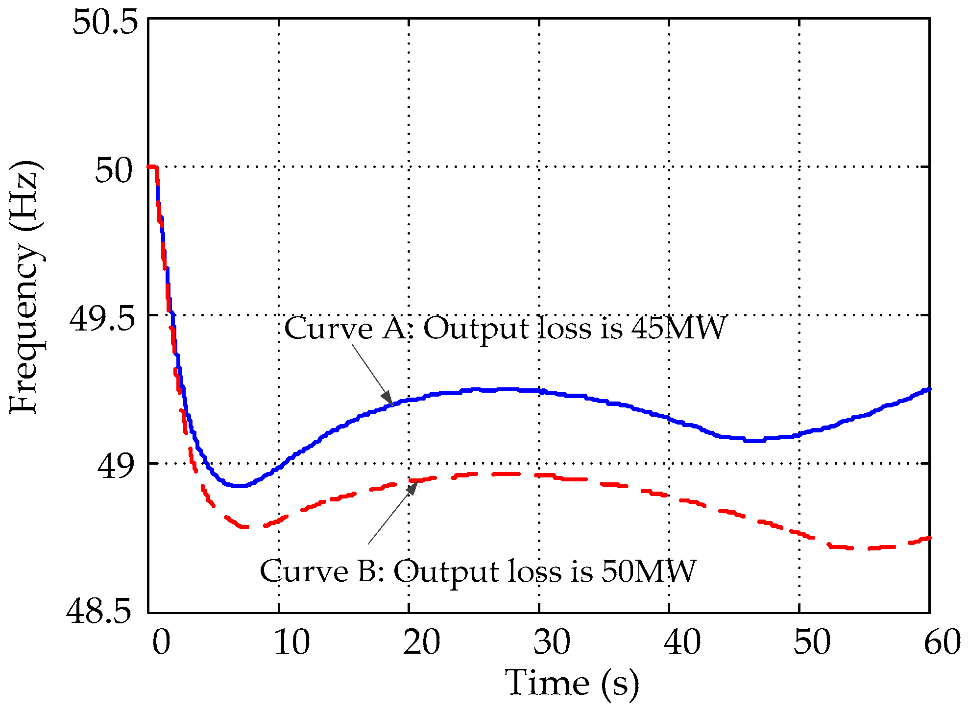
4.1. Disturbance with Single Parameter

4.1.1. Case 1: Generation Reduction in Power Plant M

Considering generation reduction in power plant M, then the TFAI under different amounts of generation can be obtained, which is shown as Curve 1 in Figure 7. Curve 1 shows that if the generation reduction is 46.70 MW, then the TFAI is 1, and the system frequency is critical acceptable, i.e., ΔP_cr = 46.70 MW. Furthermore, the TFAM η according to Equation (3) can be obtained as shown in Curve 2 of Figure 7.

Curve 2 in Figure 7 shows that, compared to TFAI, the proposed TFAM can show the degree of frequency acceptability more directly, and provide a more intuitive measure of the distance from the current operation point to the frequency collapse point. It is more convenient for the dispatcher.

4.1.2. Case 2: Load Shedding at Bus H

Considering load shedding at bus H, the TFAI under different amounts of load shedding can be obtained, which is shown as Curve 1 in Figure 8. Curve 1 shows that if the amount of load shedding is 100 MW, then the TFAI is about 1, and the system frequency is critical acceptable. That is, ΔP_cr = 100 MW. Furthermore, the TFAM according to Equation (3) can be obtained as shown in Curve 2 of Figure 8.

As shown in Figure 8, similarly to Figure 7, the TFAM can show the degree of the frequency acceptability more intuitively, and provide a more intuitive measure of the distance from the current operation point to the frequency collapse point. Hence, it is more convenient for dispatchers.

4.1.3. Case 3: Generation Reduction in Power Plant P

Considering generation reduction in power plant P, then the TFAI under different amounts of generation reduction can be obtained, which is shown as Curve 1 in Figure 9.

Curve 1 shows that when the generation reduction is 34 MW, which is the maximum generation reduction, the TFAI is about 0.039, and the system frequency deviation is still acceptable. According to Section 2.2.1, the critical disturbance power can be set as ΔP_cr = 2ΔP_max = 68 MW.

Furthermore, the TFAM η according to Equation (3) can be obtained as shown as Curve 2 of Figure 9.

Figure 9 shows that, similarly to Figure 7 and Figure 8, the proposed TFAM is more linear, can provide a more intuitive measure of the distance from the current operation point to the frequency collapse point, and is more convenient for the dispatchers.

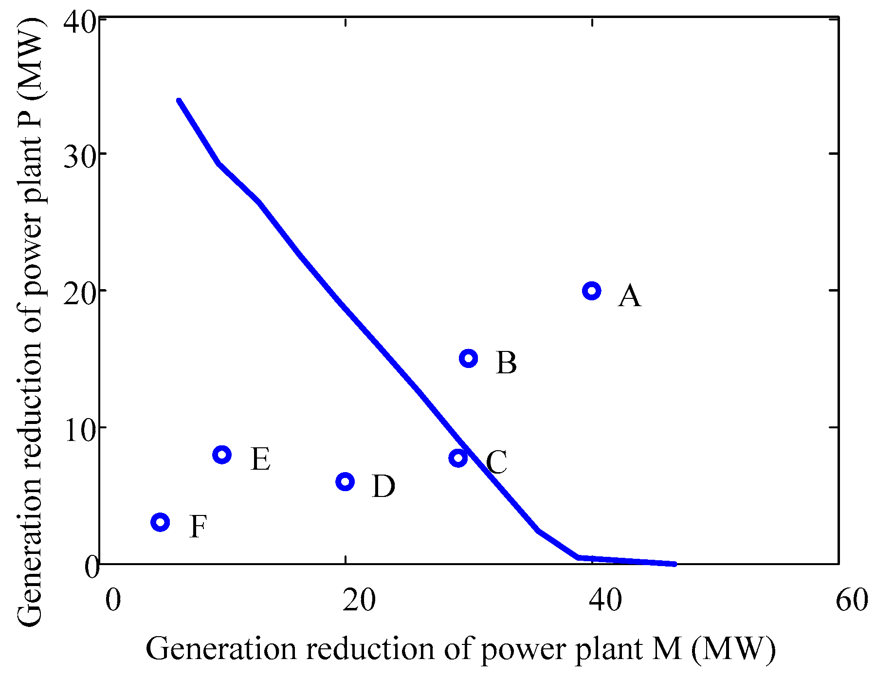
4.2. Disturbance with Multiple Parameters

Consider the disturbance involving simultaneous generation reductions at power plants M and P. With different simulations, the critical disturbances corresponding to the critical transient frequency acceptability (when F = 1) can be obtained, as shown by the solid line in Figure 10. In Figure 10, the area to the lower left of the solid line is the region where the transient frequency is acceptable, while the upper right is the region where the transient frequency is unacceptable.

Further, ΔP_dist^M and ΔP_dist^P indicate the generation reduction of the power plants M and P, respectively. If the direction of the disturbance power is fixed (ΔP_dist^M/ΔP_dist^P = const), the TFAM of the arbitrary disturbance power point can be determined by the method of Section 2.2.3. If the direction of the disturbance power is not fixed, the TFAM of any disturbance power point can be determined by the method of Section 2.2.2.

As shown in Figure 10, six disturbance power points are selected randomly, and the TFAM of these points can be obtained. The results for the random disturbances A–F are shown in Figure 10 and

Table 5. Generation reduction of two power plants and corresponding TFAM

Point Nomenclature	Generation Reduction of Power Plant M ΔPdistM/MW	Generation Reduction of Power Plant P ΔPdistP/MW	TFAM η/%
A	40	20	−46.59
B	30	15	−14.34
C	29.25	7.718	4.56
D	20	6	31.18
E	10	8	53.75
F	5	3	79.21

.

As shown in Figure 10, for the acceptable cases, the distances of the points to the critical acceptable boundary are ranked C < D < E < F. Meanwhile, the TFAM shows that C < D < E < F. Consequently, for the acceptable case, the farther the point is from the boundary, the greater the TFAM. In particular, C is close to the boundary, so the TFAM of C is close to 0.

As shown in Figure 10, for the unacceptable cases, the distances of the points to the critical acceptable boundary are ranked B < A. Meanwhile, the TFAM shows that A < B. Consequently, for the unacceptable case, the farther the point is from the boundary, the smaller the TFAM.

The above situations indicate the consistency of the TFAM and Figure 10. Similarly to Section 3.1, the TFAM can directly show the degree of the frequency acceptability, indicating the distance from the current operation point to the frequency collapse point, and is more convenient for the dispatchers.

4.3. Comparison of TFAM and Other Indexes

To determine the transient frequency stability, a transient frequency deviation index (TFDI) is proposed in [27]. The TFDI only considers the case of a frequency drop. The expression of TFDI is as follows:

$$\epsilon =\frac{S_{\mathrm{d}}}{(f_{\mathrm{N}}-f_{\mathrm{cr}})t_{\mathrm{cr}}}$$

(14)

where

$$S_{\mathrm{d}}=\min {\displaystyle {\int }_{t_{\mathrm{s}}}^{t_{\mathrm{s}}+t_{\mathrm{cr}}}(f-f_{\mathrm{cr}})dt}$$

and: f_N is the nominal frequency of the system; f_cr is the limit of frequency deviation; t_cr is the maximum acceptable duration for frequency deviation forgoing beyond f_cr; t_s is the observing window starting time; f is the frequency response.

When ε > 0, the frequency is stable; when ε < 0, the frequency is unstable; and, when ε = 0, the frequency is critical stable.

Ref. [26] also proposed a new index for frequency deviation security assessment. This index also only considers the case of a frequency drop. According to whether the frequency response curve intersects with f_cr, this index can be divided into two cases. One is if the frequency response curve intersects with f_cr. The expression is as follows:

$$\gamma =\frac{t_{\mathrm{cr}}-t_{\mathrm{b}}}{t_{\mathrm{cr}}}$$

(15)

where t_b is the continuous duration time when frequency is less than f_cr.

For Equation (15), when 0 ≤ γ≤ 1, t_b ≤ t_cr, the frequency deviation is secure. When γ < 0, t_b > t_cr, and the frequency deviation is unsecure.

The other case is that the frequency response curve does not intersect with f_cr. The expression is as follows:

$$\gamma =\frac{f_{\min }-f_{\mathrm{cr}}}{f_{\mathrm{N}}-f_{\mathrm{cr}}}+1$$

(16)

where f_min is the lowest point of the frequency response curve.

For Equation (16), γ > 1 is confirmed, and the frequency deviation must be secure.

Since both indexes ε and γ are based on a frequency threshold, we need to specify a threshold for these two indexes, and then compare them with the TFAM.

Firstly, the frequency threshold of ε is set to 48.8 Hz, and the maximum time allowed to be below the threshold is set to 0.3 s. By changing the output loss of power plant M, the TFAM and ε corresponding to each output loss can be measured. These results are shown in Figure 11. The frequency response curves when the output loss of power plant M is 45 MW and 50 MW are shown in Figure 12.

When the output loss of power plant M is 45 MW, the frequency response curve is shown as Curve A of Figure 12. At this time, the frequency meets the requirements of three thresholds, so the frequency deviation is acceptable. According to Curve 1 and Curve 2 in Figure 11, when the output loss of power plant M is 45 MW, both ε and TFAM are greater than 0, and the judgment of these two indexes is correct.

Similarly, when the output loss of power plant M is 50 MW, the frequency response curve is shown as Curve B in Figure 12. The duration when the frequency is lower than 48.8 Hz is greater than 0.3 s, so the frequency deviation is unacceptable. According to Curve 1 and Curve 2 in Figure 11, when the output loss of power plant M is 50MW, both ε and TFAM are less than 0, and the judgment of these two indexes is correct.

In addition, because ε only focuses on the threshold of 48.8 Hz, and TFAM needs to consider three thresholds, the zero-crossing positions of the two curves in Figure 11 are different.

From the above analysis, it can be seen that both ε and TFAM can correctly determine the acceptability of frequency deviation.

Second, the frequency threshold of γ is set to 49 Hz, and the maximum time allowed to be below the threshold is set to 10 s. By changing the output loss of power plant M, the TFAM and γ corresponding to each output loss can be measured. These results are shown in Figure 13.

When the output loss of power plant M is 45 MW, the frequency response curve is shown as Curve A of Figure 12. At this time, the frequency meets the requirements of three thresholds, so the frequency deviation is acceptable. According to Curve 1 and Curve 2 in Figure 13, when the output loss of power plant M is 45 MW, both γ and TFAM are greater than 0, and the judgment of these two indexes is correct.

Similarly, when the output loss of power plant M is 50 MW, the frequency response curve is shown as Curve B in Figure 12. The duration when the frequency is lower than 49 Hz is greater than 10 s, so the frequency deviation is unacceptable. According to Curve 1 and Curve 2 in Figure 13, when the output loss of power plant M is 50 MW, both γ and TFAM are less than 0, and the judgment of these two indexes is correct.

In addition, because γ only focuses on the threshold of 49 Hz, and TFAM needs to consider three thresholds, the zero-crossing positions of the two curves in Figure 13 are different.

From the above analysis, it can be seen that both γ and TFAM can correctly determine the acceptability of frequency deviation.

Compared with γ, ε and the TFAM have better linearity, and can provide a more intuitive measure of the distance from the current operation point to the frequency collapse point. It is more convenient for dispatchers to control the frequency by using these two indexes. Compared with ε, the TFAM proposed in this paper can meet the requirements of multiple frequency thresholds and have a wider range of applications.

5. Conclusions and Discussions

This paper proposes a new transient frequency acceptability margin (TFAM) based on TFAI. First, a TFAI is proposed based on the frequency trajectory and the principle that different weights correspond to different frequency deviations. The TFAI considers the frequency thresholds and time duration limits. Then, the effectiveness of the TFAI is verified by simulation. Further, the critical disturbance power is determined by using the TFAI. The TFAM is proposed to measure the distance of the actual disturbance power to the critical disturbance power. It must be noticed that the TFAM is expressed in power space and considers the power mismatch. Consequently, compared with other frequency margins, the TFAM is more convenient to formulate security control measures. The TFAM can also be used to compare the transient frequency deviation acceptability under different faults. The TFAM is convenient for dispatchers to judge the transient frequency acceptability and implement security measures in time.

There are still some problems in the TFAI and TFAM proposed in this paper. When the frequency oscillates violently, the area of integration is very small, so the TFAI is likely to fail to determine the frequency acceptability. Moreover, the critical boundary for TFAM needs to be obtained by off-line calculation. For large-scale systems, off-line calculation of the critical boundary under different operation modes and faults is time consuming. Therefore, the calculation method of the TFAI and TFAM needs further study.

References

1. Chan, M.L.; Dunlop, R.D.; Schweppe, F. Dynamic equivalents for average system frequency behavior following major disturbances. IEEE Trans. Power Appar. Syst. 1972, 91, 1637–1642. [Google Scholar] [CrossRef]
2. Kundur, P.; Paserba, J.; Ajjarapu, V.; Andersson, G.; Bose, A.; Canizares, C.; Hatziargyriou, N.; Hill, D.; Stankovic, A.; Taylor, C.; et al. Definition and classification of power system stability IEEE/CIGRE joint task force on stability terms and definitions. IEEE Trans. Power Syst. 2004, 19, 1387–1401. [Google Scholar] [CrossRef]
3. Han, Y.D.; Min, Y.; Hong, S.B. Analysis of power-frequency dynamics in large scale multi-machine power systems. Autom. Electr. Power Syst. 1992, 1, 28–33. [Google Scholar]
4. Brazil, T.J. Accurate and efficient incorporation of frequency-domain data within linear and non-linear time-domain transient simulations. In Proceedings of the IEEE MTT-S International Microwave Symposium Digest, Long Beach, CA, USA, 17 June 2005; pp. 797–800. [Google Scholar]
5. Tavakkoli, M.; Arabi, J.; Zabihi, S.; Godina, R.; Pouresmaeil, E. Reserve Allocation of Photovoltaic Systems to Improve Frequency Stability in Hybrid Power Systems. Energies 2018, 11, 2583. [Google Scholar] [CrossRef]
6. Tavakkoli, M.; Pouresmaeil, E.; Arabi, J.; Godina, R.; Catalao, J.P.S. Load-frequency control in a multi-source power system connected to wind farms through multi terminal HVDC systems. Comput. Oper. Res. 2018, 96, 305–315. [Google Scholar] [CrossRef]
7. Shehadeh, H.; Favuzza, S.; Sanseverino, E.R. Electrostatic synchronous generator model of an inverter-based distributed generators. In Proceedings of the 2015 International Conference on Renewable Energy Research and Applications (ICRERA), Palermo, Italy, 22–25 November 2015. [Google Scholar]
8. Thong, V.V.; Driesen, J.; Belmans, R. Transmission system operation concerns with high penetration level of distributed generation. In Proceedings of the 2007 42nd International Universities Power Engineering Conference, Brighton, UK, 4–6 September 2007. [Google Scholar]
9. Sapari, N.M.; Mokhlis, H.; Bakar, A.H.A.; Dahalan, M.R.M. Online stability index monitoring for load shedding scheme in islanded distribution network. In Proceedings of the 2014 IEEE 8th International Power Engineering and Optimization Conference (PEOCO2014), Langkawi, Malaysia, 24–25 March 2014; pp. 445–449. [Google Scholar]
10. Zhang, H.T.; Lai, C.S.; Lai, L.L. A novel load shedding strategy for distribution systems with distributed generations. In Proceedings of the IEEE PES Innovative Smart Grid Technologies, Europe, Istanbul, Turkey, 12–15 October 2014; pp. 1–6. [Google Scholar]
11. Zhao, Z.L.; Yang, P.; Guerrero, J.M.; Xu, Z.R.; Green, T.C. Multiple-Time-Scales Hierarchical Frequency Stability Control Strategy of Medium-Voltage Isolated Microgrid. IEEE Trans. Power Electron. 2015, 31, 5974–5991. [Google Scholar] [CrossRef]
12. Velez, F.G.; Centeno, V.A.; Phadke, A.G. Multiple swing transient stability assessment with phasor measurements. In Proceedings of the IEEE Manchester Power Tech, Manchester, UK, 18–22 June 2017. [Google Scholar]
13. Wu, Z.Y.; Zora, L.T.; Phadke, A.G. Simultaneous transmission line parameter and PMU measurement calibration. In Proceedings of the IEEE Power & Energy Society General Meeting, Denver, CO, USA, 26–30 July 2015. [Google Scholar]
14. Abdal-Rahman, K.; Mill, L.; Phadke, A.G.; De La Ree, J.; Liu, Y.L. Internet based wide area information sharing and its roles in power system state estimation. In Proceedings of the IEEE Power Engineering Society Winter Meeting, Columbus, OH, USA, 28 January–1 February 2001. [Google Scholar]
15. Larsson, M.; Christian, R. Predictive frequency stability control based on wide-area phase measurements. In Proceedings of the IEEE Power Engineering Society Summer Meeting, Chicago, IL, USA, 21–25 July 2002; Volume 1, pp. 233–238. [Google Scholar]
16. Thorp, J.S.; Wang, X.R.; Hopkinson, K.M. Agent technology applied to the protection of power systems. In Autonomous Systems and Intelligent Agents in Power System Control and Operation; Springer: Berlin, Germany, 2003; pp. 115–154. ISBN 978-3540402022. [Google Scholar]
17. Zhang, W.; Wang, X.R.; Liao, G.D. Automatic load shedding emergency control algorithm of power system based on wide-area measurement data. Power Syst. Technol. 2009, 33, 69–73. [Google Scholar] [CrossRef]
18. Chen, C.R.; Liu, C.C. Dynamic stability assessment of power system using a new supervised clustering algorithm. In Proceedings of the 2000 Power Engineering Society Summer Meeting, Seattle, WA, USA, 16–20 July 2000; pp. 1851–1854. [Google Scholar]
19. Rahmann, C.; Ortiz-Villalba, D.; Alvarez, R.; Salles, M. Methodology for selecting operating points and contingencies for frequency stability studies. In Proceedings of the 2017 IEEE Power and Energy Society General Meeting, Chicago, IL, USA, 16–20 July 2017; pp. 1–5. [Google Scholar]
20. YatendraBabu, G.V.N.; Naguru, N.R.; Sarkar, V. Real-Time Transient Instability Detection Using Frequency Trend Vector in Wide Area Monitoring System. In Proceedings of the 2016 IEEE 6th International Conference on Power Systems (ICPS), New Delhi, India, 4–6 March 2016; pp. 1–4. [Google Scholar]
21. Seethalekshmi, K.; Singh, S.N.; Srivastava, S.C. WAMS assisted frequency and voltage stability based adaptive load shedding scheme. In Proceedings of the 2009 IEEE Power and Energy Society General Meeting, Calgary, AB, Canada, 26–30 July 2009; pp. 1–8. [Google Scholar]
22. Ye, H.; Qi, Z.P.; Pei, W. Modeling and evaluation of short-term frequency control for participation of wind farms and energy storage in power systems. In Proceedings of the 2014 International Conference on Power System Technology, Chengdu, China, 20–22 October 2014; pp. 2647–2654. [Google Scholar]
23. Xu, T.S.; Xue, Y.S. Quantitative analysis of acceptability of transient frequency offset. Autom. Electr. Power Syst. 2002, 19, 7–10. [Google Scholar]
24. Xu, T.S.; Li, B.J.; Bao, Y.H. Global optimization of UFLS and UVLS quantity considering transient safety. Autom. Electr. Power Syst. 2003, 22, 12–15. [Google Scholar]
25. Liu, H.T.; Zeng, Y.G.; Li, J.S. UFLS scheme based on frequency security quantitative analysis for China Southern Power Grid. Electr. Power 2007, 40, 28–32. [Google Scholar]
26. Zhang, H.X.; Liu, Y.T. New index for frequency deviation security assessment. In Proceedings of the 2010 Conference Proceedings IPEC, Singapore, 27–29 October 2010; pp. 1031–1034. [Google Scholar]
27. Iessa, A.; Wahab, N.I.A.; Mariun, N.; Hizam, H. Method of estimating the maximum penetration level of wind power using transient frequency deviation index based on COI frequency. In Proceedings of the 2016 IEEE International Conference on Power and Energy (PECon), Melaka, Malaysia, 28–29 November 2016; pp. 274–279. [Google Scholar]
28. Zhang, H.X.; Hou, Z.Y.; Liu, Y.T. Online Security Assessment of Power System Frequency Deviation. In Proceedings of the 2012 Asia-Pacific Power and Energy Engineering Conference, Shanghai, China, 27–29 March 2012; pp. 1–4. [Google Scholar]
29. Liu, Y.T.; Li, C.G. Impact of large-scale wind penetration on transient frequency stability. In Proceedings of the 2012 IEEE Power and Energy Society General Meeting, San Diego, CA, USA, 22–26 July 2012; pp. 1–5. [Google Scholar]
30. Sun, Y.K. Study on the Third Line Defense of Frequency Stability Coordinating Control for Sending-End Power System. Master’s Dissertation, North China Electrical Power University, Beijing, China, 11 March 2014. [Google Scholar]
31. Tan, F. Study on Frequency Stability Coordinating Control for Sending-End Power System with the Integration of Large-Scale Wind Power. Master’s Dissertation, North China Electrical Power University, Beijing, China, 11 March 2014. [Google Scholar]
32. Yue, L.; Xue, A.C.; Cui, J.H. Study on the influence of transient frequency Evaluation Index and governor parameter of small power grid. Power Syst. Technol. 2018, 42, 4031–4036. [Google Scholar] [CrossRef]
33. Xue, A.C.; Wu, F.F.; Lu, Q.; Mei, S.W. Power system dynamic security region and its approximation. IEEE Trans. Circuits Syst. I Regul. Papers 2006, 53, 2849–2859. [Google Scholar] [CrossRef]
34. Kaye, R.J.; Wu, F.F. Dynamic security regions of power systems. IEEE Trans. Circuits Syst. 1982, 29, 612–623. [Google Scholar] [CrossRef]
35. Chinese National Energy Administration. DL/T 1234-2013 Technique Specification of Power System Security and Stability Calculation; China Electric Power Press: Beijing, China, 2013; pp. 15–16.
Figure 1. Frequency band division of transient frequency acceptability index (TFAI).
Energies 12 00012 g001
Figure 2. Weighted quantitative analysis of frequency.
Energies 12 00012 g002
Figure 3. The case that a disturbance involves two parameters.
Energies 12 00012 g003
Figure 4. The topology of small grid Z.
Energies 12 00012 g004
Figure 5. Frequency trajectories under the disturbance A.
Energies 12 00012 g005
Figure 6. Frequency trajectories under different disturbances.
Energies 12 00012 g006
Figure 7. TFAI and transient frequency acceptability margin (TFAM) corresponding to different generation reductions.
Energies 12 00012 g007
Figure 8. TFAI and TFAM corresponding to different load shedding quantities.
Energies 12 00012 g008
Figure 9. TFAI and TFAM corresponding to different generation reduction of power plant P.
Energies 12 00012 g009
Figure 10. Critical acceptable boundary with respect to generation reduction of two power plants.
Energies 12 00012 g010
Figure 11. Generation reduction of power plant M and the corresponding TFAM and ε.
Energies 12 00012 g011
Figure 12. Frequency response curves when the output loss of power plant M is 45 MW and 50 MW.
Energies 12 00012 g012
Figure 13. Generation reduction of power plant M and corresponding TFAM and γ.
Energies 12 00012 g013