Formal Asymptotic Analysis of Online Scheduling Algorithms for Plug-In Electric Vehicles’ Charging

Abstract

A large-scale integration of plug-in electric vehicles (PEVs) into the power grid system has necessitated the design of online scheduling algorithms to accommodate the after-effects of this new type of load, i.e., PEVs, on the overall efficiency of the power system. In online settings, the low computational complexity of the corresponding scheduling algorithms is of paramount importance for the reliable, secure, and efficient operation of the grid system. Generally, the computational complexity of an algorithm is computed using asymptotic analysis. Traditionally, the analysis is performed using the paper-pencil proof method, which is error-prone and thus not suitable for analyzing the mission-critical online scheduling algorithms for PEV charging. To overcome these issues, this paper presents a formal asymptotic analysis approach for online scheduling algorithms for PEV charging using higher-order-logic theorem proving, which is a sound computer-based verification approach. For illustration purposes, we present the complexity analysis of two state-of-the-art online algorithms: the Online cooRdinated CHARging Decision (ORCHARD) algorithm and online Expected Load Flattening (ELF) algorithm.

1. Introduction

Electric road technologies are envisaged as alternatives to traditional fossil-fuel-based transportation due to their low greenhouse gas emissions, energy security, and noise mitigation. These advantages have led to a rapid increase in their volume, e.g., more than 1 million electric vehicles were sold worldwide in the year 2017 alone [1]. This enormous increase has also resulted in a new billion-dollar industry for the development and deployment of electric vehicle (EV) units and their operations [2].

Plug-in electric vehicles (PEVs) are a type of electric vehicle and are characterized by a comparatively larger battery, a charging plug, and an internal combustion engine for powering the vehicle and battery [3]. This technology, in conjunction with the smart grid concept, enables the bidirectional flow of power, i.e., from the grid to the vehicle and from the vehicle to the grid [4]. The use of electric vehicles as a load that can be scheduled in the electricity system, offering storage capability and bidirectional power flow, is anticipated to be effectively used as part of the integration of renewable energy sources, load flattening, peak shaving, and frequency fluctuation mitigation [5]. Therefore, the optimal scheduling of PEV charging/discharging results in an optimized bidirectional flow of power between PEVs and power grid [6], and thus, a reduced capital cost of electricity generation and minimization of the operational cost of the grid.

Mathematically, the PEV scheduling problem for charging/discharging is posed as an optimization problem subject to the constraints imposed by the infrastructure and physical properties of the grid and EVs. The optimization problem is then solved using linear programming [7], nonlinear programming [8], model predictive control (MPC) [9], and queuing theory [10], among many other methods. These scheduling algorithms are further classified as online and offline algorithms, which provide scheduling based on causal and non-causal information, respectively.

In an offline setting, a PEV’s charging profile is assumed to be known to the charging station for scheduling purposes, prior to the arrival of the PEV [11,12]. However, in real-world settings, the assumption of prior knowledge is not realistic. Moreover, the PEV charging problem is prone to the uncertainties introduced by the random arrival and departure of PEVs, intermittent power generation from renewable energy sources, and fluctuation in demand and prices of the electricity in the system [5]. In this context, online algorithms cater to the uncertainties associated with the PEV charging problem. In an online setting, the arrival and departure times and charging demand of a PEV are only available to the controller for purposes of scheduling when a PEV is plugged into the charging facility. The scheduler then schedules all the plugged-in PEVs and also allocates the charging rate to each PEV so that the objectives, such as power consumption, are minimized, as shown in Figure 1.

Generally, an online algorithm incorporates information based on the history, knowledge, and statistics available for the future data, in addition to the currently available data, to improve the overall efficiency of the algorithm [13]. Although the use of an online scheduling algorithm for PEV charging facilitates the account of uncertainties, the efficiency of these algorithms is highly sensitive to the size of the PEV population. A large population of PEVs results in exponential growth of the computational complexity of these algorithms which, in turn, can jeopardize the reliability, efficiency, and security of the grid operation. To address this issue, recent online scheduling algorithms have alleviated the unbearable computational cost of the online algorithms by devising various low-complexity routines for the optimal scheduling of PEVs [9,14,15].

The computational complexity of an algorithm refers to the number of primitive operations or steps required to solve a given task using some method or an algorithm [16]. These primitive operations include basic arithmetic operations, such as addition, subtraction, multiplication, and division. In the study of algorithm analysis, a pseudocode is usually used to describe the working of an algorithm using control structures adopted from different conventional programming languages and mathematical notations. The computational complexity for a given algorithm can be judged based on the number of steps from the pseudocode of the given algorithm and also the cost associated with each step. Mathematically, the computational complexity utilizes asymptotic theory, which, by definition, characterizes the limiting behavior of a function [17], with respect to the input size, to describe the notions of the best, worst, and average case computational complexity of an algorithm [16]. Asymptotic notations, such as Big-Oh (Big-O), Big-Omega (Big-$\mathrm{\Omega }$), Big-Theta (Big-$\mathrm{\Theta }$), little-oh (little-o), and little-omega (little-$\omega$), are used to express the asymptotic bounds for the complexity function of a given algorithm, and thus allows us to characterize the efficiency of an algorithm and also compare relative performance of alternative algorithms [16].

Table 1. Asymptotic Notations.

Notation	Limit Definition	Set Definition
$f=O\left(g\right)$	$\underset{n\to \infty }{lim}\frac{f\left(n\right)}{g\left(n\right)}\ne \infty$	$\left\{f\left(n\right)\right|(\exists c{n}_o.(\forall n_o<n\wedge 0<c\Rightarrow \left|f\left(n\right)\right|\le cg\left(n\right)\left)\right)\}$
$f=\mathrm{\Omega }\left(g\right)$	$\underset{n\to \infty }{lim}\frac{f\left(n\right)}{g\left(n\right)}\ne 0$	$\left\{f\left(n\right)\right|(\exists c{n}_o.(\forall n_o<n\wedge 0<c\Rightarrow cg\left(n\right)\le \left|f\left(n\right)\right|\left)\right)\}$
$f=\mathrm{\Theta }\left(g\right)$	$\underset{n\to \infty }{lim}\frac{f\left(n\right)}{g\left(n\right)}\ne 0,\infty$	$\left\{f\left(n\right)\right|\exists c_1{c}_2{n}_o.(\forall n_o<n\wedge 0<c_1\wedge 0<c_2\Rightarrow c_{1}g\left(n\right)\le \left|f\left(n\right)\right|\le c_{2}g\left(n\right)\left)\right)\}$
$f=o\left(g\right)$	$\underset{n\to \infty }{lim}\frac{f\left(n\right)}{g\left(n\right)}=0$	$\left\{f\left(n\right)\right|(\exists c{n}_o.(\forall n_o<n\wedge 0<c\Rightarrow \left|f\left(n\right)\right|<cg\left(n\right)\left)\right)\}$
$f=\omega \left(g\right)$	$\underset{n\to \infty }{lim}\frac{f\left(n\right)}{g\left(n\right)}=\infty$	$\left\{f\left(n\right)\right|(\exists c{n}_o.(\forall n_o<n\wedge 0<c\Rightarrow cg\left(n\right)<\left|f\left(n\right)\right|\left)\right)\}$

presents the asymptotic notions in terms of limits and set theory.

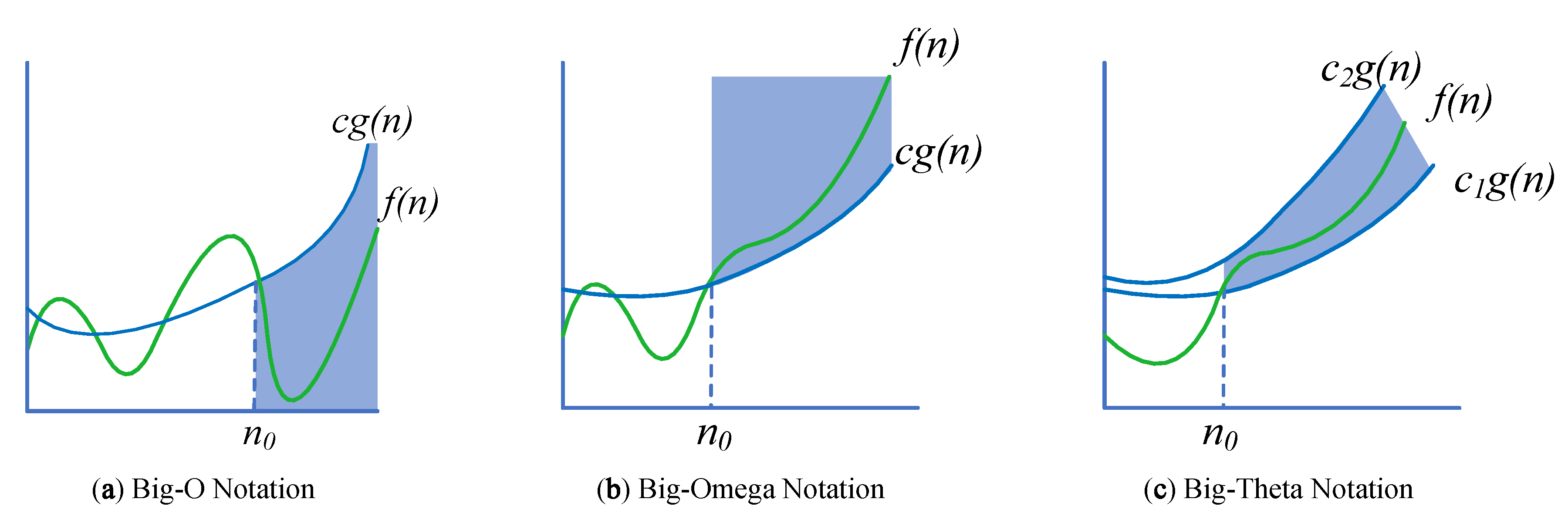
Big-O is a set that contains all functions, $f\left(n\right)$, for which there always exist constants $n_o$ and c, such that the magnitude of $f\left(n\right)$ is less than and equal to the constant multiplier of function $g\left(n\right)$, i.e., $f\left(n\right)\le cg\left(n\right)$, for some $n_o<n$, as shown in Figure 2a. Big-O allows for describing the upper bound of a function and, therefore, it is used to abstract the worst-case running time or space complexity of an algorithm.

Big-$\mathrm{\Omega }$ is a set that contains all functions $f\left(n\right)$, for which there always exist constants $n_o$ and c, such that the magnitude of $f\left(n\right)$ is greater than and equal to the constant multiplier of the function $g\left(n\right)$, i.e., $cg\left(n\right)\le f\left(n\right)$, for some $n_o<n$, as shown in Figure 2b. Big-$\mathrm{\Theta }$ is a set that contains all functions $f\left(n\right)$, for which there always exist constants $n_o$, $c_1$, and $c_2$, such that the magnitude of $f\left(n\right)$ is bounded by the constant multiplier of function $g\left(n\right)$, i.e., $c_{1}g\left(n\right)\le f\left(n\right)\le c_{2}g\left(n\right)$, for some $n_o<n$, as shown in Figure 2c. This notation is used for describing the situation when an algorithm has the same best- or worst-case computational or space complexity. To the contrary, little-o and little-$\omega$ are used to describe weak asymptotic lower and upper bounds by not incorporating the equality condition used in the definitions of the Big-O and Big-$\mathrm{\Omega }$, respectively.

Traditional analysis techniques, such as simulations and computer algebra systems, cannot be used to conduct a complete asymptotic analysis of algorithms due to their inability to deal with the limiting behavior, as shown in Table 1, in a true manner. Therefore, in practice, the asymptotic analysis is carried out using the paper-pencil method. However, it is also error-prone due to the involvement of humans in the analysis. Moreover, this analysis method is not scalable, as the large-sized models cannot be handled very efficiently on paper. To address these issues, we propose to use a formal asymptotic analysis technique for the online scheduling algorithms for PEV charging schedules.

Formal methods [18] are computer-based mathematical techniques, which are being widely adopted for the specification, analysis, and verification of hardware and software systems. These techniques use logic to formally express and reason with regard to the mathematical models of systems and, therefore, they provide a mechanized platform which is characterized as highly expressive and sound [19]. A suitable logic, such as temporal logic, first-order, predicate, and second- or higher-order logic, with the help of its well-defined syntax, semantics, and proof theory, allows for expressing a discrete or continuous model of the given system and formally reasoning and verifying the correctness of the intended behavior of the system based upon a few axioms of the corresponding logic. A combination of logic and modeling technique, such as finite state machine (FSM) and automaton, leads to a variety of formal method-based solutions [20] for the formal verification of systems, such as sequential or concurrent systems.

Formal methods can be mainly categorized into two mainstream techniques, i.e., model checking and theorem proving techniques. Model checking [21] employs the finite state machine notion to model the system for the purpose of exhaustive state-space verification of systems in a model checker—a piece of software. Model checking allows automatic verification and thus is easy to use, but it can be subject to state-space explosion for the systems—a situation when the state-space of the corresponding model grows extremely large. Moreover, model checking cannot be used to verify generic mathematical expressions and, therefore, it is not suitable to formally model and verify properties regarding asymptotic notations, which are based upon the limits concept. On the other hand, theorem proving is a formal methods technique that allows for describing any mathematical model by choosing an appropriate logic and then using mathematical reasoning to verify its corresponding properties in a theorem prover—a piece of software. Higher-order logic is quite expressive and allows reasoning about continuous aspects as well. Therefore, we employed theorem proving for the formal asymptotic analysis of online scheduling algorithms for PEV charging.

The primary objective of this paper is to develop a framework for the formal asymptotic analysis using theorem proving for online charging scheduling algorithms for plug-in electric vehicles. A rigorous formal verification of the computational complexity of algorithms results in the explicit specification of assumptions under which results will be valid. These assumptions are about the system parameters, such as number of vehicles, etc., and, therefore, are helpful in providing valuable insights before the implementation phase. Moreover, due to the generic formalization of asymptotic notations, the formalization can be utilized readily for the applications of asymptotic analysis in many other fields, such as applied mathematics and probability theory. The O-notation has been formalized in the Isabelle/HOL (higher-order-logic) theorem prover [22] using the ring theory. However, to the best of our knowledge, this formalization of asymptotic notations has not been used to analyze any practical problem. Moreover, to the best of our knowledge, the other asymptotic notations, i.e., Big-$\mathrm{\Omega }$, Big-$\mathrm{\Theta }$, little-o, and little-$\omega$, have not been formalized in higher-order logic. In this paper, we propose a real theory-based formalization of all asymptotic notations using the HOL-Light theorem prover and utilize them to analyze the computational complexity of online scheduling algorithms for PEV charging.

Keeping in view the uncertainties coupled to the electric vehicle charging scheduling problem, various online algorithms are available in the literature to alleviate negative effects and harvest potential benefits from the integration of this new type of load into the grid system. For example, an online auction protocol to increase the allocation efficiency of a charging facility in comparison to a fixed price strategy, given the requirements of electric vehicle owners, is described in [15]. Similarly, a decentralized [6,11] approach is used for optimally allocating a charging or discharging schedule to plugged-in electric vehicles for the purpose of using the electricity stored in the mounted batteries with a low computational burden on the central utility. However, the aforementioned approaches require beforehand knowledge of electric vehicle charging demands, which may not be always available. The nonlinear online maximum sensitivity selection-based charging algorithm (NOL-MSSCA) [23] is used to cater to the current harmonic effects caused by the injection of variable speed drives (VSDs), variable frequency drives (VFDs), energy-efficient lights, switching converters, smart appliances, and plug-in electric vehicles (PEVs) in the grid system. NOL-MSSCA considers the random arrival of PEVs into the system over the span of 24 h and uses a priority-based criterion for allocating resources for charging electric vehicles to minimize the effects of current harmonics caused by nonlinear loads. However, this work does not address the computational complexity issue explicitly. The Online cooRdinated CHARging Decision (ORCHARD) algorithm [9] models an online scenario by considering random arrivals or departures of electric vehicles and their charging demands. Moreover, a low computational complexity routine is devised to avoid computational burden for solving the scheduling problem of PEVs for every arrival or departure. There is another class of load scheduling algorithms which rely on the model predictive control (MPC) approach to utilize future information of the load to enhance the grid operation and achieve various desirable objectives, like energy cost and uncertainty regulation [14,24,25,26]. In particular, Expected Load Flattening (ELF) [14] is based on the assumption of random arrivals or departures of PEVs along with additional future information, incorporated using a model predictive approach, for an optimal online scheduling of PEV charging.

The algorithms, i.e., ORCHARD and ELF, besides being state-of-the-art, claim to reduce the worst-case computational complexity of the scheduling algorithms for PEV charging. However, the existing computational complexity analysis of these algorithms is based on the traditional paper-and-pencil proof method and is quite informal in its presentation, as well. On the other hand, the computational complexity of online algorithms is usually a foremost consideration for the appropriate and efficient functioning of the real-time systems [27], as a high computational complexity can lead to an unbearable monetary loss in a PEV integrated grid system. Therefore, in this paper, we present the formal verification of the computational complexity of the aforementioned algorithms using the formalization of asymptotic notations in HOL-Light. Besides the formal verification of asymptotic properties in the sound core of HOL-Light, the main challenge involved in the proposed work is the formulation of the mathematical problem—related to the complexity of the given algorithms—for conducting their formal analysis in the HOL-Light theorem prover.

1.1. Contribution of the Paper

The main contributions of this paper are:

• A higher-order-logic framework is proposed to conduct formal asymptotic analysis using the HOL-Light theorem prover.
• Formal verification of low computational complexity results are reported for state-of-the-art online scheduling algorithms for PEV charging, i.e., ORCHARD and ELF.
• The formally verified low computational complexity results are then used to compare the effect of the cost of operation of a scheduler and PEV load for ORCHARD and ELF algorithms in MATLAB R2016a [28].

1.2. Organization of the Paper

The rest of the paper is organized as follows: Section 2 describes some preliminaries essential for the understanding of the rest of the paper. Section 3 provides the methodology adopted to formally analyze the online scheduling algorithms for PEV charging. Section 4 describes the formalization of asymptotic notations in HOL-Light. Section 5 describes the formal analysis of the chosen algorithms in HOL-Light. Finally, Section 6 concludes the paper.

2. Preliminaries

This section provides a brief introduction to theorem proving and HOL-Light theorem prover to facilitate the understanding of the rest of the paper.

2.1. Theorem Proving

Theorem proving is a widely used formal method [18] for describing and verifying the mathematical model of a system using formal logic, such as propositional, first-order, and second- or higher-order logic. A well-defined proof theory, semantics, and syntax of the formal logic allows the rigorous reasoning of the system’s design, properties, and correctness [29]. Various theorem provers, e.g., HOL-Light [30], HOL [31], Coq [32], and PVS [33], have been used for the mechanization of the formal proofs.

Theorem proving is mainly categorized as automated and interactive theorem proving. In automated theorem proving, a decidable logic is employed to model the system, and, therefore, it is possible to develop automatic procedures for the verification of the model. However, the limited expressiveness of the decidable logic does not allow for modeling complex mathematical notions, such as limits, which are commonly employed to analyze the system’s behavior. Therefore, a more expressive formal logic, such as higher-order logic, is used to model such behaviors. These logical frameworks, however, require interaction between humans and machines to accomplish the verification task of the system. Generally, this type of theorem proving is referred to as interactive theorem proving. The ability to use a wide range of logic in the verification process makes theorem proving a highly expressive and flexible technique for formal verification.

Theorem proving provides a very flexible platform for the abstraction, formal verification, and specification of mathematical concepts, such as the limiting behavior of functions, and, therefore, we chose this technique for the formal asymptotic analysis of the online scheduling algorithms for PEV charging.

2.2. HOL-Light Theorem Prover

HOL-Light [30] is an interactive higher-order-logic theorem prover that belongs to the HOL family of theorem provers. The higher-order logic is implemented using Objective CAML (OCaml) language [34]—which is a variant of the strongly typed functional programming language—in HOL-Light to express and apply proof strategies and develop logical theories. HOL-Light provides formal reasoning support for many mathematical theories, including sets, natural numbers, real analysis, complex analysis, and vector calculus, and has been particularly successful in verifying many software and hardware systems [18,30,35].

HOL-Light provides a platform for the secure and sound formal verification and specification of systems under verification. Secure theorem proving is ensured because of its small core, which consists of 1500 lines, including a core set of 10 primitive inference rules, such as modus ponens and reflexivity. These primitive inferences are realized as OCaml language, and every new theorem is proved using these rules. These verified theorems can be stored for future use as an HOL-Light theory, which is a computer file. These theories can be loaded by the HOL-Light users in their running sessions, and, therefore, they can be utilized for the verification of new theorems. HOL-Light supports both backward and forward proof methods. The former consists of using inference rules to deduce the proof of the desired theorem, whereas the latter consists of breaking the main goal into subgoals using HOL-Light tactics, which are special ML functions for generating subgoals from a main goal.

We selected the HOL-Light theorem prover for the proposed work as it is equipped with a rich library of mathematical theories of set, natural numbers, and real numbers.

Table 2. Higher-order-logic (HOL) symbols and functions.

HOL Symbol	Standard Symbol	Meaning
∧	$and$	Logical $and$
∨	$or$	Logical $or$
¬	$not$	Logical $negation$
$\lambda \mathtt{x}.\mathtt{t}$	$\lambda x.t$	Function that maps x to $t\left(x\right)$
$\mathtt{num}$	$\{0,1,2,\dots \}$	Positive integers data type
$\mathtt{real}$	All real numbers	Real data type
$\mathtt{SUC}\mathtt{n}$	$n+1$	Successor of a $num$
$\mathtt{rpow}\mathtt{x}\mathtt{y}$	$x^y$	Power with real exponent
$\mathtt{max}\left(\mathtt{f}\right(\mathtt{x}),\mathtt{g}(\mathtt{x}\left)\right)$	$max\left(g\right(x),f(x\left)\right)$	Maximum among $f\left(x\right)$ and $g\left(x\right)$

presents some frequently used HOL-Light functions and symbols to facilitate the understanding of the formalization and verification in this paper.

3. Proposed Methodology

In this section, we present the main steps of the proposed methodology, depicted in Figure 3, for conducting the formal asymptotic analysis of online scheduling algorithms for PEV charging.

• As a first step, we formalize asymptotic notations in higher-order logic to be able to formally verify the properties of asymptotic notations in the sound core of the HOL-Light theorem prover. The formalization is based on the formalized mathematical theories of set, real, and natural number theories available in the library of HOL-Light. This formalization allows the formal verification of the properties of asymptotic notations, which play a pivotal role in the formal verification of the results related to the online scheduling algorithms for PEV charging.
• The second step in the formal asymptotic analysis of an algorithm for PEVs is to represent its behavior while incorporating its implicit concepts as a pseudocode. As described earlier, this pseudocode then forms the basis on which we can describe the complexity function of an algorithm afterward. Due to the very generic and flexible presentations of algorithms, availability in the PEV literature, and varying audiences, it is not a very easy task to obtain the pseudocodes of the available algorithms. For example, the pseudocode for the Online cooRdinated CHARging Decision (ORCHARD) algorithm, considered in this paper for the formal asymptotic analysis, is not available in the original paper [9]. Moreover, this step also allows the explicit investigation and specification of the pseudocodes of ancillary algorithms (such as insertion sort algorithm) which are required to accomplish the formal analysis of online scheduling algorithms for PEV charging.
• Finally, the computational complexity functions obtained from Step 2 are formally specified as higher-order-logic functions, utilizing the formal modeling of asymptotic notations from Step 1. Then, the properties of interest for an algorithm are formally verified as higher-order-logic theorems using the sound core of the HOL-Light theorem prover based on the formalized notions and properties of asymptotic notations from Step 1, as shown in Figure 3.

4. Formalization of Asymptotic Notations in HOL-Light

In this section, we present a higher-order-logic formalization of asymptotic notations, described in Table 1, in the HOL-Light theorem prover.

Definition 1.

$⊢\forall \mathtt{g}.\mathtt{BigO}(\mathtt{g}:\mathtt{num}\to \mathtt{real})=$

$$\begin{array}{c}\left\{\right(\mathtt{f}:\mathtt{num}\to \mathtt{real}\left)\right|(\exists \mathtt{c}\mathtt{n}\_\mathtt{0}.(\forall \mathtt{n}.\mathtt{n}\_\mathtt{0}\le \mathtt{n}\hfill \\ \hfill \Rightarrow \mathtt{0}<\mathtt{c}\wedge \mathtt{0}\le \mathtt{f}\left(\mathtt{n}\right)\wedge \mathtt{f}\left(\mathtt{n}\right)\le \mathtt{c}\ast \mathtt{g}\left(\mathtt{n}\right)\left)\right)\}\end{array}$$

where $\mathtt{g}:\mathtt{num}\to \mathtt{real}$ and $\mathtt{f}:\mathtt{num}\to \mathtt{real}$ are functions that accept a natural number ($\mathtt{num}$) as an argument and return a real number ($\mathtt{real}$). The constants $\mathtt{c}$ and $\mathtt{n}\_\mathtt{0}$ are of type $\mathtt{real}$ and $\mathtt{num}$, respectively, and $\mathtt{n}$ is a variable of type ($\mathtt{num}$). $\mathtt{BigO}$ is a higher-order-logic function that accepts a function $\mathtt{g}:\mathtt{num}\to \mathtt{real}$ as an argument and returns a set of functions such that every $\mathtt{f}$ has a growth rate proportional to the product of function $\mathtt{g}$ and a constant multiplier $\mathtt{c}$, i.e., $\mathtt{0}\le \mathtt{f}\left(\mathtt{n}\right)\le \mathtt{c}\ast \mathtt{g}\left(\mathtt{n}\right)$. On the other hand, $\mathtt{0}\le \mathtt{f}\left(\mathtt{n}\right)$ ensures that the member function is a positive function. In algorithm analysis, Big-O notation is used to specify the asymptotic upper bound for the complexity of an algorithm.

Definition 2.

$⊢\forall \mathtt{g}.\mathtt{BigOmega}(\mathtt{g}:\mathtt{num}\to \mathtt{real})=$

$\left\{\right(\mathtt{f}:\mathtt{num}\to \mathtt{real}\left)\right|(\exists \mathtt{c}\mathtt{n}\_\mathtt{0}.(\forall \mathtt{n}.\mathtt{n}\_\mathtt{0}\le \mathtt{n}$$\Rightarrow \mathtt{0}<\mathtt{c}\wedge \mathtt{0}\le \mathtt{c}\ast \mathtt{g}\left(\mathtt{n}\right)\le \mathtt{f}\left(\mathtt{n}\right)\left)\right)\}$

In the above definition, $\mathtt{BigOmega}$ is a higher-order-logic function that accepts a function $\mathtt{g}:\mathtt{num}\to \mathtt{real}$ as an argument and returns a set of functions such that every $\mathtt{f}$ has a growth rate proportional to the product of function $\mathtt{g}$ and a constant multiplier $\mathtt{c}$, i.e., $\mathtt{0}\le \mathtt{c}\ast \mathtt{g}\left(\mathtt{n}\right)\le \mathtt{f}\left(\mathtt{n}\right)$. On the other hand, $\mathtt{0}\le \mathtt{f}\left(\mathtt{n}\right)$ ensures that the member function is a positive function. In algorithm analysis, Big-$\mathrm{\Omega }$ notation is used to specify the asymptotic lower bound for the complexity of an algorithm.

Definition 3.

$⊢\forall \mathtt{g}.\mathtt{BigTheta}(\mathtt{g}:\mathtt{num}\to \mathtt{real})=$

$$\begin{array}{c}\left\{\right(\mathtt{f}:\mathtt{num}\to \mathtt{real}\left)\right|(\exists \mathtt{c}\mathtt{1}\mathtt{c}\mathtt{2}\mathtt{n}\_\mathtt{0}.(\forall \mathtt{n}.\mathtt{n}\_\mathtt{0}\le \mathtt{n}\hfill \\ \hfill \Rightarrow \mathtt{0}<\mathtt{c}\mathtt{1}\wedge \mathtt{0}<\mathtt{c}\mathtt{2}\wedge \mathtt{0}\le \mathtt{c}\mathtt{1}\ast \mathtt{g}\left(\mathtt{n}\right)\le \mathtt{f}\left(\mathtt{n}\right)\le \mathtt{c}\mathtt{2}\ast \mathtt{g}\left(\mathtt{n}\right)\left)\right)\}\end{array}$$

In the above definition, $\mathtt{BigTheta}$ is a higher-order-logic function that accepts a function $\mathtt{g}:\mathtt{num}\to \mathtt{real}$ as an argument and returns a set of functions such that every $\mathtt{f}$ growth rate satisfies an inequality, i.e., $\mathtt{c}\mathtt{1}\ast \mathtt{g}\left(\mathtt{n}\right)\le \mathtt{f}\left(\mathtt{n}\right)\le \mathtt{c}\mathtt{2}\ast \mathtt{g}\left(\mathtt{n}\right)$, where $\mathtt{c}\mathtt{1}$ and $\mathtt{c}\mathtt{2}$ are real constants. In algorithm analysis, Big-$\mathrm{\Theta }$ notation is used to specify the asymptotic tight bounds for the complexity of an algorithm.

Definition 4.

$⊢\forall \mathtt{g}.\mathtt{LittleO}(\mathtt{g}:\mathtt{num}\to \mathtt{real})=$

$$\begin{array}{c}\left\{\right(\mathtt{f}:\mathtt{num}\to \mathtt{real}\left)\right|(\exists \mathtt{c}\mathtt{n}\_\mathtt{0}.(\forall \mathtt{n}.\mathtt{n}\_\mathtt{0}\le \mathtt{n}\hfill \\ \hfill \Rightarrow \mathtt{0}\le \mathtt{c}\wedge \mathtt{0}<\mathtt{f}\left(\mathtt{n}\right)\wedge \mathtt{f}\left(\mathtt{n}\right)<\mathtt{c}\ast \mathtt{g}\left(\mathtt{n}\right)\left)\right)\}\end{array}$$

In the above definition, $\mathtt{LittleO}$ is a higher-order-logic function that accepts a function $\mathtt{g}:\mathtt{num}\to \mathtt{real}$ as an argument and returns a set of functions such that every $\mathtt{f}$ growth rate is less than the multiple of a constant $\mathtt{c}$ and function $\mathtt{g}$, i.e., $\mathtt{f}\left(\mathtt{n}\right)<\mathtt{c}\ast \mathtt{g}\left(\mathtt{n}\right)$. In algorithm analysis, little-o notation is used to specify the strict asymptotic upper bound for the complexity of an algorithm.

Definition 5.

$⊢\forall \mathtt{g}.\mathtt{LittleOmega}(\mathtt{g}:\mathtt{num}\to \mathtt{real})=$

$\left\{\right(\mathtt{f}:\mathtt{num}\to \mathtt{real}\left)\right|(\exists \mathtt{c}\mathtt{n}\_\mathtt{0}.(\forall \mathtt{n}.\mathtt{n}\_\mathtt{0}\le \mathtt{n}$$\Rightarrow \mathtt{0}<\mathtt{c}\wedge \mathtt{0}\le \mathtt{c}\ast \mathtt{g}\left(\mathtt{n}\right)<\mathtt{f}\left(\mathtt{n}\right)\left)\right)\}$

In the above definition, $\mathtt{LittleOmega}$ notation is a higher-order-logic function that accepts a function $\mathtt{g}:\mathtt{num}\to \mathtt{real}$ as an argument and returns a set of functions such that the growth rate of every function is greater than the multiple of a constant $\mathtt{c}$ and function $\mathtt{g}$, i.e., $\mathtt{c}\ast \mathtt{g}\left(\mathtt{n}\right)<\mathtt{f}\left(\mathtt{n}\right)$.

In algorithm analysis, little-$\omega$ notation is used to specify the strict asymptotic lower bound for the complexity of an algorithm.

The above definitions in higher-order logic enable the reasoning of the correctness of their properties in HOL-Light.

Formal Verification of Asymptotic Notations’ Properties

In this subsection, we present the formally verified properties of the asymptotic notations in HOL-Light, based on the formal definitions given in the previous section.

We first present the formally verified theorems corresponding to the transitivity property of the asymptotic notations:

Theorem 1.

$⊢\forall \mathtt{f}\mathtt{g}\mathtt{h}.,\mathtt{f}\in \mathtt{BigO}\mathtt{g}\wedge \mathtt{g}\in \mathtt{BigO}\mathtt{h}\Rightarrow \mathtt{f}\in \mathtt{BigO}\mathtt{h}$

Theorem 2.

$⊢\forall \mathtt{f}\mathtt{g}\mathtt{h}.$

$\mathtt{f}\in \mathtt{BigOmega}\mathtt{g}\wedge \mathtt{g}\in \mathtt{BigOmega}\mathtt{h}\Rightarrow \mathtt{f}\in \mathtt{BigOmega}\mathtt{h}$

Theorem 3.

$⊢\forall \mathtt{f}\mathtt{g}\mathtt{h}.$

$\mathtt{f}\in \mathtt{BigTheta}\mathtt{g}\wedge \mathtt{g}\in \mathtt{BigTheta}\mathtt{h}\Rightarrow \mathtt{f}\in \mathtt{BigTheta}\mathtt{h}$

Theorem 4.

$⊢\forall \mathtt{f}\mathtt{g}\mathtt{h}.$

$\mathtt{f}\in \mathtt{Littelo}\mathtt{g}\wedge \mathtt{g}\in \mathtt{Littelo}\mathtt{h}\Rightarrow \mathtt{f}\in \mathtt{Littelo}\mathtt{h}$

Theorem 5.

$⊢\forall \mathtt{f}\mathtt{g}\mathtt{h}.$

$\mathtt{f}\in \mathtt{Littelomega}\mathtt{g}\wedge \mathtt{g}\in \mathtt{Littelomega}\mathtt{h}\Rightarrow \mathtt{f}\in \mathtt{Littelomega}\mathtt{h}$

In Theorems 1–5, $\mathtt{f}$, $\mathtt{g}$, and $\mathtt{h}$ are functions that accept an argument of type $\mathtt{num}$ and return a real number. The transitivity property formally verifies the asymptotic relationship of two functions $\mathtt{f}$ and $\mathtt{h}$, given that their asymptotic relationship with function $\mathtt{g}$ is valid.

Next, we present the formally verified results for the reflexivity property of the Big-O, Big-$\mathrm{\Omega }$, and Big-$\mathrm{\Theta }$:

Theorem 6.

$⊢\forall \mathtt{f}.(\exists {\mathtt{n}}_{\mathtt{0}}.(\forall \mathtt{m}.{\mathtt{n}}_{\mathtt{0}}\le \mathtt{m}\Rightarrow \mathtt{0}\le \mathtt{f}\mathtt{m})\Rightarrow (\mathtt{f}\in \mathtt{BigO}\mathtt{f}))$

Theorem 7.

$⊢\forall \mathtt{f}.(\exists {\mathtt{n}}_{\mathtt{0}}.(\forall \mathtt{m}.{\mathtt{n}}_{\mathtt{0}}\le \mathtt{m}\Rightarrow \mathtt{0}\le \mathtt{f}\mathtt{m})\Rightarrow (\mathtt{f}\in \mathtt{BigOmega}\mathtt{f}))$

Theorem 8.

$⊢\forall \mathtt{f}.(\exists {\mathtt{n}}_{\mathtt{0}}.(\forall \mathtt{m}.{\mathtt{n}}_{\mathtt{0}}\le \mathtt{m}\Rightarrow \mathtt{0}\le \mathtt{f}\mathtt{m})\Rightarrow (\mathtt{f}\in \mathtt{BigTheta}\mathtt{f}))$

In the above theorems, $\mathtt{f}$ and $\mathtt{g}$ are functions that accept a number $\mathtt{num}$ as an argument and return a real number. Theorems 6–8 are formally verified results which depict that any function $\mathtt{f}$ is asymptotically related to itself for Big-O, Big-$\mathrm{\Omega }$, and Big-$\mathrm{\Theta }$ notations.

The next property is related to the summation of the Big-O and Big-$\mathrm{\Omega }$ notations and is formally verified as:

Theorem 9.

$⊢\forall \mathtt{t}\mathtt{1}\mathtt{t}\mathtt{2}\mathtt{g}\mathtt{1}\mathtt{g}\mathtt{2}.$

$(\mathtt{t}\mathtt{1}\in \mathtt{BigO}\mathtt{g}\mathtt{1})\wedge (\mathtt{t}\mathtt{2}\in \mathtt{BigO}\mathtt{g}\mathtt{2})$

$\Rightarrow ($$\lambda \mathtt{n}.\mathtt{t}\mathtt{1}\mathtt{n}+\mathtt{t}\mathtt{2}\mathtt{n})\in (\mathtt{BigO}\left(\mathtt{max}\right(\mathtt{g}\mathtt{1},\mathtt{g}\mathtt{2}\left)\right)$

Theorem 10.

$⊢\forall \mathtt{t}\mathtt{1}\mathtt{t}\mathtt{2}\mathtt{g}\mathtt{1}\mathtt{g}\mathtt{2}.$

$(\mathtt{t}\mathtt{1}\in \mathtt{BigOmega}\mathtt{g}\mathtt{1})\wedge (\mathtt{t}\mathtt{2}\in \mathtt{BigOmega}\mathtt{g}\mathtt{2})$

$\Rightarrow ($$\lambda \mathtt{n}.\mathtt{t}\mathtt{1}\mathtt{n}+\mathtt{t}\mathtt{2}\mathtt{n})\in (\mathtt{BigOmega}\left(\mathtt{min}\right(\mathtt{g}\mathtt{1},\mathtt{g}\mathtt{2}\left)\right)$

In the above theorems, $\mathtt{t}\mathtt{1}$, $\mathtt{t}\mathtt{2}$, $\mathtt{g}\mathtt{1}$, and $\mathtt{g}\mathtt{2}$ are functions that accept an argument of type $\mathtt{num}$ and return a real value. Theorem 9 formally verifies the fact that if two functions $\mathtt{t}\mathtt{1}$ and $\mathtt{t}\mathtt{2}$ are in the Big-O of $\mathtt{g}\mathtt{1}$ and $\mathtt{g}\mathtt{2}$, respectively, then the sum of these two functions will also be in the Big-O of the maximum of the $\mathtt{g}\mathtt{1}$ and $\mathtt{g}\mathtt{2}$ functions. It is due to the fact that the Big-O notation provides an upper asymptotic bound for a function. Similarly, the sum of two functions $\mathtt{t}\mathtt{1}$ and $\mathtt{t}\mathtt{2}$, which are in the Big-$\mathrm{\Omega }$ of $\mathtt{g}\mathtt{1}$ and $\mathtt{g}\mathtt{2}$, will be in the Big-$\mathrm{\Omega }$ of the minimum of the $\mathtt{g}\mathtt{1}$ and $\mathtt{g}\mathtt{2}$ functions. This is also due to the fact that Big-$\mathrm{\Omega }$ provides a lower asymptotic bound for a function.

Next, we present the formally verified symmetry property of the Big-$\mathrm{\Omega }$ and Big-$\mathrm{\Theta }$ notations:

Theorem 11.

$⊢\forall \mathtt{f}\mathtt{g}.$$\mathtt{f}\in \mathtt{BigOmega}\mathtt{g}\Rightarrow \mathtt{g}\in \mathtt{BigOmega}\mathtt{f}$

Theorem 12.

$⊢\forall \mathtt{f}\mathtt{g}.$$\mathtt{f}\in \mathtt{BigTheta}\mathtt{g}\Rightarrow \mathtt{g}\in \mathtt{BigTheta}\mathtt{f}$

In the above theorems, $\mathtt{f}$ and $\mathtt{g}$ are functions that accept an argument of type $\mathtt{num}$ and return a real number. Theorems 11 and 12 formally verify that if the growth rate of a function $\mathtt{f}$ is related to a function $\mathtt{g}$ through the Big-$\omega$ or Big-$\mathrm{\Theta }$ notations, then the growth rate of $\mathtt{g}$ will also be related to $\mathtt{f}$ through Big-$\omega$ or Big-$\mathrm{\Theta }$.

Next, we present the formally verified transpose symmetry property:

Theorem 13.

$⊢\forall \mathtt{f}\mathtt{g}.$$\mathtt{f}\in \mathtt{BigO}\mathtt{g}\Rightarrow \mathtt{g}\in \mathtt{BigOmega}\mathtt{f}$

Theorem 14.

$⊢\forall \mathtt{f}\mathtt{g}.$$\mathtt{f}\in \mathtt{Littelo}\mathtt{g}\Rightarrow \mathtt{g}\in \mathtt{LittleOmega}\mathtt{f}$

In the above theorems, $\mathtt{f}$ and $\mathtt{g}$ are functions that accept an argument of type $\mathtt{num}$ and return a real number. Theorem 13 formally verifies that a function $\mathtt{f}$ whose growth rate is related to the function $\mathtt{g}$ through Big-O notations will also satisfy the Big-$\mathrm{\Omega }$ relationship between function $\mathtt{g}$ and $\mathtt{f}$. Similarly, Theorem 14 is formally verified for the functions related through little-o and little-$\omega$.

Moreover, as the Big-O notation plays a vital role in the formal verification of online scheduling algorithms for PEV charging, two frequently used properties of the Big-O notation are also verified.

Theorem 15.

$⊢\forall \mathtt{f}\mathtt{g}.$$\mathtt{f}\in \mathtt{BigO}\mathtt{g}\Rightarrow \forall \mathtt{k}.($$\lambda \mathtt{n}.\mathtt{k}\ast \mathtt{f}\mathtt{n})\in (\mathtt{BigO}\mathtt{g})$

Theorem 15, formally verifies that for a function $\mathtt{f}$ whose growth rate is in the Big-O of a function $\mathtt{g}$, then a scalar ($\mathtt{k}$) multiplication will not affect the relationship.

Theorem 16.

$⊢\forall \mathtt{t}\mathtt{1}\mathtt{t}\mathtt{2}\mathtt{g}\mathtt{1}\mathtt{g}\mathtt{2}.$

$(\mathtt{t}\mathtt{1}\in \mathtt{BigO}\mathtt{g}\mathtt{1})\wedge (\mathtt{t}\mathtt{2}\in \mathtt{BigO}\mathtt{g}\mathtt{2})$

$\Rightarrow ($$\lambda \mathtt{n}.\mathtt{t}\mathtt{1}\mathtt{n}\ast \mathtt{t}\mathtt{2}\mathtt{n})\in (\mathtt{BigO}(\mathtt{g}\mathtt{1}\ast \mathtt{g}\mathtt{2}))$

On the other hand, $\mathtt{t}\mathtt{1}$, $\mathtt{t}\mathtt{2}$, $\mathtt{g}\mathtt{1}$, and $\mathtt{g}\mathtt{2}$ are functions that accept an argument of type num and return a real number. Theorem 16 formally verifies that if two functions $\mathtt{t}\mathtt{1}$ and $\mathtt{t}\mathtt{2}$ are in O($\mathtt{g}\mathtt{1}$) and O($\mathtt{g}\mathtt{2}$), respectively, then their multiplication will belong to the set O($\mathtt{g}\mathtt{1}\ast \mathtt{g}\mathtt{2}$).

The above formalization allows for formally reasoning and verifying the computational complexity of an algorithm. For this paper, we particularly use these results for the formal verification of the online scheduling algorithms for PEV charging.

5. Formal Asymptotic Analysis of Scheduling Algorithms for PEVs

In this section, we present the formally verified results for the worst-case computational complexity of the insertion sort algorithm, Online cooRdinated CHARging Decision (ORCHARD) [9] and online Expected Load Flattening (ELF) algorithms [14].

5.1. Formal Analysis of Insertion Sort Algorithm

Sorting is a process of listing the items in some logical order, such as ascending, descending, alphabetical, chronological, or even topological. There are many computer applications where sorting is employed, such as searching, information retrieval, crunching, and data mining. Therefore, there are a number of algorithms designed to accomplish the task, such as insertion sort, mergesort, heapsort, counting sort, quicksort, and radix sort [16]. As the computational complexities of the algorithms, selected as case studies in this paper, are originally computed using the insertion sort algorithm, the formal analysis of these online scheduling algorithms, in this paper, is also based on the insertion sorting algorithm. For a given input, the algorithm picks each entry and sorts the order of the entry for a segment of input up to that entry and places it according to its desired logical order. The algorithm repeats the procedure for all the entries of the input until the desired order is achieved [16]. The computational complexity of the algorithm is the function of the input length n and has an $O\left(n^2\right)$ worst-case asymptotic bound [16].

Algorithm 1 is a pseudocode describing the working of the algorithm [16]. It accepts a list of objects—in our case, the information related to PEVs—for sorting its entries in an ascending order. In Line 1, the FOR loop is used to perform sorting of the entries of the list, where n is the total length of the input list $\mathit{A}$. The loop executes n times, and $c_1$ is the cost associated to each execution of the FOR loop statement. In Line 2, the current entry of the list is assigned as a $key$, which is a local variable used for sorting a particular entry. The execution cost for this statement is considered $c_2$ and it runs for $n-1$ times as the body of a FOR or WHILE loop runs one time less than the loop statement. Next, in Line 3, a local variable i is assigned the value of $j-1$, and the execution cost of this statement is considered $c_3$ and it runs for $n-1$ times as well. In Line 4, the WHILE loop is used to perform the comparison test on the subarray $A[1,\dots ,i]$. This test expression is executed ${\sum }_{j=2}^n{t}_j$ times with an execution cost of $c_4$ for each run, where $t_j$ is the number of times the WHILE loop runs for the comparison of a specific $key$. The expressions in the body of WHILE, i.e., Lines 5 and 6, are executed ${\sum }_{j=2}^n{t}_j-1$ times. Line 5 shifts the entry to one place in the right direction in the list $\mathit{A}$, given the conditions in the WHILE loop are satisfied. Then, Line 6 updates the entry of the subarray for the comparison in the next iteration of the WHILE loop, where $c_5$ and $c_6$ are the costs for each execution of these expressions. Finally, the $key$ is updated for the next iteration of the FOR loop in Line 7. The expression is also executed $n-1$ times with a cost of $c_7$ for each execution. The algorithm outputs a sorted array A in ascending order. The running time complexity function $T\left(n\right)$ is obtained by multiplying the cost of each execution, i.e., $c_i$, with the total time steps each statement is expected to take in the procedure of sorting, and then summing all of these products.

$$T\left(n\right)=c_{1}n+c_2(n-1)+c_3(n-1)+c_4\sum _{j=2}^n{t}_j$$

$$+c_5\sum _{j=2}^n(t_j-1)+c_6\sum _{j=2}^n(t_j-1)+c_7(n-1)$$

In the worst case, the steps of an algorithm are executed the maximum possible number of times by the algorithm for performing the intended task.

$$T\left(n\right)=(\frac{c_4}{2}+\frac{c_5}{2}+\frac{c_6}{2})n^2-(c_1+c_2+c_3+\frac{c_4}{2}+\frac{c_5}{2}$$

$$+\frac{c_6}{2}+c_7)n-(c_2+c_3+c_4+c_7)$$

Algorithm 1 Insertion Sort	Cost	Time Steps
Input: list $\mathit{A}$
1: for $j=2$ to n	$c_1$	n
2: $\mathit{key}=A\left[j\right]$	$c_2$	$n-1$
3: $i=j-1$	$c_3$	$n-1$
4: while $i>0$ and $A\left[i\right]>key$	$c_4$	${\sum }_{j=2}^n{t}_j$
5:   $A[i+1]=A\left[i\right]$	$c_5$	${\sum }_{j=2}^n(t_j-1)$
6:   $i=i-1$	$c_6$	${\sum }_{j=2}^n(t_j-1)$
7: $A[i+1]=\mathit{key}$	$c_7$	$n-1$

The worst-case running time for an insertion sort algorithm is defined in higher-order logic as:

Definition 6.

$⊢\forall \mathtt{n}\mathtt{c}\mathtt{1}\mathtt{c}\mathtt{2}\mathtt{c}\mathtt{3}\mathtt{c}\mathtt{4}\mathtt{c}\mathtt{5}\mathtt{c}\mathtt{6}\mathtt{c}\mathtt{7}.$

$$\begin{array}{c}\mathtt{i}\_\mathtt{sort}\_\mathtt{wc}\_\mathtt{t}\mathtt{n}\mathtt{c}\mathtt{1}\mathtt{c}\mathtt{2}\mathtt{c}\mathtt{3}\mathtt{c}\mathtt{4}\mathtt{c}\mathtt{5}\mathtt{c}\mathtt{6}\mathtt{c}\mathtt{7}=\hfill \\ (\frac{\mathtt{c}\mathtt{4}}{\mathtt{2}}++\frac{\mathtt{c}\mathtt{5}}{\mathtt{2}}+\frac{\mathtt{c}\mathtt{6}}{\mathtt{2}})\mathtt{n}\mathtt{pow}\mathtt{2}-({\mathtt{c}}_{\mathtt{1}}+{\mathtt{c}}_{\mathtt{2}}+{\mathtt{c}}_{\mathtt{3}}\\ \hfill +\frac{\mathtt{c}\mathtt{4}}{\mathtt{2}}+\frac{\mathtt{c}\mathtt{5}}{\mathtt{2}}+\frac{\mathtt{c}\mathtt{6}}{\mathtt{2}}+\mathtt{c}\mathtt{7})\mathtt{n}-(\mathtt{c}\mathtt{2}+\mathtt{c}\mathtt{3}+\mathtt{c}\mathtt{4}+\mathtt{c}\mathtt{7})\end{array}$$

where $\mathtt{c}\mathtt{1}$, $\mathtt{c}\mathtt{2}$, $\mathtt{c}\mathtt{3}$, $\mathtt{c}\mathtt{4}$, $\mathtt{c}\mathtt{5}$, $\mathtt{c}\mathtt{6}$, and $\mathtt{c}\mathtt{7}$ are real constants that represent the cost of performing the corresponding steps in the sorting algorithm, and $\mathtt{n}$ is the variable of type $\mathtt{num}$ representing the length of the input list A.

Definitions 1–6 and the formally verified properties of the Big-O notation in Section 4 are used to formally verify the computational complexity results for the insertion sort algorithm as follows:

Theorem 17.

$⊢\forall \mathtt{n}\mathtt{c}\mathtt{1}\mathtt{c}\mathtt{2}\mathtt{c}\mathtt{3}\mathtt{c}\mathtt{4}\mathtt{c}\mathtt{5}\mathtt{c}\mathtt{6}\mathtt{c}\mathtt{7}.$

$\mathtt{0}<\mathtt{n}\wedge \mathtt{0}<\mathtt{c}\mathtt{1}\wedge \mathtt{0}<\mathtt{c}\mathtt{2}\wedge \mathtt{0}<\mathtt{c}\mathtt{3}\wedge$

$\mathtt{0}<\mathtt{c}\mathtt{4}\wedge \mathtt{0}<\mathtt{c}\mathtt{5}\wedge \mathtt{0}<\mathtt{c}\mathtt{6}\wedge \mathtt{0}<\mathtt{c}\mathtt{7}$

$\Rightarrow ($$\lambda \mathtt{n}.\mathtt{i}\_\mathtt{sort}\_\mathtt{wc}\_\mathtt{t}\mathtt{n}\mathtt{c}\mathtt{1}\mathtt{c}\mathtt{2}\mathtt{c}\mathtt{3}\mathtt{c}\mathtt{4}\mathtt{c}\mathtt{5}\mathtt{c}\mathtt{6}\mathtt{c}\mathtt{7}\in \mathtt{BigO}\mathtt{n}\mathtt{pow}\mathtt{2})$

In the above theorem, $\mathtt{0}<\mathtt{n}$ ensures that the list is not empty, whereas $\mathtt{0}<{\mathtt{c}}_{\mathtt{i}}$ ensures that the execution cost associated with each expression is also not zero. Under these conditions, the above theorem formally verifies that the worst-case computational complexity of the insertion sort algorithm is $O\left(n^2\right)$.

Definition 6 and Theorem 17 play a vital role in the formal reasoning and verification of the computational complexity results of the online scheduling algorithms for PEV charging in the next sections.

5.2. Online cooRdinated CHARging Decision (ORCHARD)

The “Online cooRdinated CHARging Decision (ORCHARD) algorithm” [9] considers the random arrivals and departures of PEVs with random charging demands. The problem is formulated as a convex optimization problem, which is a special class of mathematical optimization problems and provides efficient and reliable optimal solutions due to its fairly complete theory [36], and it utilizes the speed scaling technique [37] to optimally schedule the charging demands of PEVs. Speed scaling is a power management technique that is widely used in computer and communication systems to reduce energy consumption. In the seminal work by Yao et al. [37], the speed scaling problem is cast as a scheduling problem in which the tasks, along with the release time, deadline, and amount of work, are not only scheduled but also allocated processor speed. Yao et al. also presented two online algorithms, i.e., average rate (AVR) and optimal available (OA), which learn about the tasks when they are available. The AVR runs each task at an average speed, which in itself is a function of the workload and time required to process the job, whereas OA schedules each task while assuming no task in the future. The ORCHARD uses a variant of the OA algorithm, i.e., qOA [38], which improves the results obtained from the OA algorithm. The ORCHARD algorithm solves the convex optimization problem of charging PEVs whenever a PEV arrives or departs using the interior point method. The computational complexity of the interior point method increases exponentially with an increase in input size. To cater to this issue, the authors in [9] presented a low-complexity algorithm to reduce the exponential computational complexity involved in the optimization problem.

The low-complexity routine in [9] exploits the structure of the optimal solution, i.e., an optimization technique such as the interior point method essentially balances the total workload for an optimal solution. Therefore, the proposed low-complexity routine balances the workload by considering the interval density to quantify the amount of the workload in the respective intervals and then shifts the load from high-density intervals to the adjacent interval with a low-density workload to balance the workload, which results in the optimal solution.

Figure 4 depicts a worst-case scenario for an online scheduling problem for PEV charging. In the worst-case scenario, the scheduler records N PEVs’ information at any time t, which consists of their arrival and departure times ($a_i$ and $f_i$, respectively) and charging demands $d_i$, for scheduling purposes. In the worst-case scenario, when there are N PEVs at time t, with arrival and departure times and charging demands to be scheduled, then there can be at most N possible intervals $I_i$. These N intervals can, at most, lead to $N^2$ possible adjacent intervals for load shifting $w_i$, termed as time windows [9], as shown in Figure 4.

Algorithm 2 describes the main computational steps of the low-complexity routine. The data required for the PEV low-complexity charging scheduling algorithm is the input, i.e., a set P, a certain time interval $\tau$, workload density ${\rho }_i$ of each time window, and $S_{\tau }$. P is the set of PEVs; $\tau \in W:=w_1,\dots ,w_{N^2}$ is a member of the set W, whose members represent all possible time windows; ${\rho }_i=\frac{1}{{\delta }_{\tau }}{\sum }_{P_i\in S_{\tau }}{d}_i$ is the density of the workload of time window $\tau$, which has length ${\delta }_{\tau }$; $S_{\tau }\in P$ is the set representing the number of PEVs in time window $\tau$. In Line 1, a WHILE loop is used that repeats the procedure until all the PEVs are scheduled. For the worst case, it is assumed that the maximum number of PEVs, i.e., N, are to be scheduled at anytime t, and, therefore, in the worst-case scenario, the loop executes N times. In Line 2, a certain time interval $\tau$ of highest workload is calculated and selected. This task can be accomplished using any sorting algorithm; however, we considered the commonly used insertion sort algorithm, described above. For N PEVs, there could be, at most, $N^2$ such time slots which are needed to be sorted and, therefore, for $n=N^2$, it has a $O\left(N^4\right)$ worst-case computational complexity, as mentioned in Algorithm 2. The sorting procedure depends on the input, and, therefore, it is imparted to the computational cost of any algorithm, which justifies its inclusion in the complexity analysis of the online scheduling algorithm.

Algorithm 2 Low-complexity Routine	Worst-case
Input:$P:=P_1,\dots ,P_N$, $\tau$, ${\rho }_{\tau }=\frac{1}{{\delta }_{\tau }}{\sum }_{P_i\in S_{\tau }}{d}_i$, $S_{\tau }\in P$
1: while $P\ne \left\{\right\}$	N
2: Determine the time interval, $\tau$ of the
highest intensity, i.e., ${\rho }_{\tau }$	$O\left(N^4\right)$
3: Allocate the charging rate, $\widehat{x_i}$, to all PEVs
such that ${\rho }_{\tau }={\sum }_{P_i\in S_{\tau }}\widehat{x_i}$
4: Set P:= $P\setminus S_I$
5: Remove I from the time horizon
and update the departure, arrival
and residual demands

Line 3 assigns to every PEV a charging rate such that the total charging rate is bounded by the maximum charging rate of the interval. In Lines 4 and 5, the algorithm removes the interval and PEVs, which are scheduled, and updates the information for the next iteration. From Lines 3 to 5, the computational cost is not taken into account due to the fact that the complexity associated with these steps is not proportional to the input size. The resulting running time function for the algorithm is then described in HOL-Light as:

Definition 7.

$⊢\forall \mathtt{N}\mathtt{c}\mathtt{1}\mathtt{c}\mathtt{2}\mathtt{c}\mathtt{3}\mathtt{c}\mathtt{4}\mathtt{c}\mathtt{5}\mathtt{c}\mathtt{6}\mathtt{c}\mathtt{7}.$

$\mathtt{lcr}\_\mathtt{wc}\_\mathtt{t}\mathtt{N}\mathtt{c}\mathtt{1}\mathtt{c}\mathtt{2}\mathtt{c}\mathtt{3}\mathtt{c}\mathtt{4}\mathtt{c}\mathtt{5}\mathtt{c}\mathtt{6}\mathtt{c}\mathtt{7}=$

$\mathtt{N}\ast \mathtt{i}\_\mathtt{sort}\_\mathtt{wc}\_\mathtt{t}\mathtt{N}\mathtt{pow}\mathtt{2}\mathtt{c}\mathtt{1}\mathtt{c}\mathtt{2},\mathtt{c}\mathtt{3}\mathtt{c}\mathtt{4}\mathtt{c}\mathtt{5}\mathtt{c}\mathtt{6}\mathtt{c}\mathtt{7}$

Definition 7 is a higher-order-logic description of the worst-case computational time of the low-complexity algorithm for execution. N represents the number of times a WHILE loop is executed for the worst-case scenario. The constants $\mathtt{c}\mathtt{1}$, $\mathtt{c}\mathtt{2}$, $\mathtt{c}\mathtt{3}$, $\mathtt{c}\mathtt{4}$, $\mathtt{c}\mathtt{5}$, $\mathtt{c}\mathtt{6}$, $\mathtt{c}\mathtt{7}$, and $\mathtt{c}\mathtt{8}$ represent the cost associated with each step in the insertion sort algorithm, whereas ${\mathtt{N}}^{\mathtt{2}}$ denotes the maximum number of intervals that are possible in the worst-case scenario. The above definition is based on the function $\mathtt{i}\_\mathtt{sort}\_\mathtt{wc}\_\mathtt{t}$ to incorporate the computational complexity due to sorting procedure in Algorithm 2.

Definitions 1, 6, and 7, along with the theorems related to the insertion sort algorithm, i.e., Theorem 17, and the formally verified properties of the Big-O notation, given in Section 4, allow us to formally verify the worst-case complexity result for the ORCHARD algorithm in HOL-Light as follows:

Theorem 18.

$⊢\forall \mathtt{N}\mathtt{c}\mathtt{1}\mathtt{c}\mathtt{2}\mathtt{c}\mathtt{3}\mathtt{c}\mathtt{4}\mathtt{c}\mathtt{5}\mathtt{c}\mathtt{6}\mathtt{c}\mathtt{7}.$

$\mathtt{0}<\mathtt{N}\wedge \mathtt{0}<\mathtt{c}\mathtt{1}\wedge \mathtt{0}<\mathtt{c}\mathtt{2}\wedge \mathtt{0}<\mathtt{c}\mathtt{3}$

$\wedge \mathtt{0}<\mathtt{c}\mathtt{4}\wedge \mathtt{0}<\mathtt{c}\mathtt{5}\wedge \mathtt{0}<\mathtt{c}\mathtt{6}\wedge \mathtt{0}<\mathtt{c}\mathtt{7}$

$\Rightarrow \mathtt{lcr}\_\mathtt{wc}\_\mathtt{t}\mathtt{N}\mathtt{c}\mathtt{1}\mathtt{c}\mathtt{2}\mathtt{c}\mathtt{3}\mathtt{c}\mathtt{4}\mathtt{c}\mathtt{5}\mathtt{c}\mathtt{6}\mathtt{c}\mathtt{7}\in \mathtt{BigO}\mathtt{N}\mathtt{pow}\mathtt{5}$

The application of theorem proving, in this case, requires us to explicitly add all the required specifications of assumptions under which the result holds true in the above theorem. For example, the precondition on the number of intervals, i.e., $\mathtt{0}<\mathtt{N}$, in Theorem 16, is added to ensure that the number of intervals is not zero, which is essential for the scheduling task. On the other hand, the preconditions on the constants originate from the formalization of the worst-case scenario of the insertion sort algorithm, presented in the previous section.

5.3. Low-Complexity Online Expected Load Flattening (ELF) Algorithm

The PEV charging scheduling problem has been formulated using the model predictive control (MPC) approach by incorporating first-order statistics of the load on the grid in [14]. This enables accounting for the potential uncertainties in the arrival and departure of PEVs to and from a charging facility and the variation in the electricity load in the grid system. The online algorithm, in [14], considers that the entire system is divided into T equal-length intervals, as shown in Figure 5.

The remaining charging demand of a PEV i which arrives at time k is defined as ${\widehat{d}}_i^k=d_i-{\sum }_{t=a_i}^{k-1}{x}_{it}$. For the PEVs that have not arrived by time $k-1$, the remaining charging demand is considered to be equal to the charging demand of that PEV, i.e., ${\widehat{d}}_i^k=d_i$. The total unfinished charging demand at time slot k is defined as the sum of remaining charging demands of all the PEVs, ${\tilde{d}}_t^k={\sum }_{i\in \left\{i\right|f_i=t\}}{\widehat{d}}_i^k,\forall t.k,\dots ,T$. The total unfinished charging demand is, then, used to define the state of the system at time t as [14]

$${\mathbf{D}}_t=[l_t,{\tilde{d}}_t^t,{\tilde{d}}_{t+1}^t,\dots ,{\tilde{d}}_T^t]$$

(1)

where $l_t$ represents the electricity demand excluding the PEV charging at time t. ${\tilde{d}}_{t^{{}^{\prime }}}^t$ is the total unfinished charging demand at time t that must be completed by time $t^{{}^{\prime }}$. Moreover, future load demands at random arrival events, ${\xi }_t$, are represented as [14]

$${\xi }_t=[{\iota }_t,{\gamma }_t^t,{\gamma }_{t+1}^t,\dots ,,{\gamma }_T^t]$$

(2)

where ${\iota }_t$ represents the base load at time t and ${\gamma }_{t^{{}^{\prime }}}^t$ represents the total unfinished charging demand that arrives at time t and must be fulfilled by time $t^{{}^{\prime }}$. Finally, the first-order statistics of ${\xi }_t$ are represented as

$${ϵ}_t=[{\alpha }_t,{\beta }_t^t,{\beta }_{t+1}^t,\dots ,,{\beta }_T^t]$$

(3)

where ${\alpha }_t=\mathrm{E}\left[{\iota }_t\right]$ and ${\beta }_{t^{{}^{\prime }}}^t=\mathrm{E}\left[{\gamma }_{t^{{}^{\prime }}}^t\right]$ are the expected values for the random variables representing base load and total unfinished charging demands, respectively. The algorithm, using the state of the system (1) and first-order statistical data (3) at every time slot, finds the near-optimal solution, $s_k^{*}$, with respect to the offline solution, $r^{*}$, to the optimization problem described in [14], as shown in Figure 5. Conventionally, numerical methods, such as the interior point methods, are employed to find the solution at each stage k, which leads to an unbearable computational cost, especially in the case of the large-scale integration of the PEVs with the grid system. Therefore, the authors in [14] used a low-complexity Expected Load Flattening (ELF) algorithm to reduce the computational complexity.

The ELF algorithm relies on the load flattening characteristic of the optimal solution, i.e., the standard numerical methods try to flatten the demand curve. Therefore, the ELF algorithm tries to balance the charging demand among all the time slots $k,\dots ,T$, where T denotes total time stages in the problem, to flatten the charging demand curve of PEVs. The ELF charging scheduling algorithm incorporates the information of (1) and (3) in ${\overline{d}}_{t^{{}^{″}}}^{t^{{}^{\prime }}}$

$${\overline{d}}_{t^{{}^{″}}}^t=\{\begin{array}{cc}{\tilde{d}}_{t^{{}^{″}}}^{t^{{}^{\prime }}},\hfill & \mathrm{for}{t}^{{}^{″}}=k,\dots ,T,t^{{}^{\prime }}=k\hfill \\ {\beta }_{t^{{}^{″}}}^{t^{{}^{\prime }}},\hfill & \mathrm{for}{t}^{{}^{″}}=t^{{}^{\prime }},\dots ,T,t^{{}^{\prime }}=k+1,\dots ,T\end{array}$$

(4)

Algorithm 3 provides the pseudocode of the ELF algorithm that describes the procedure and computational steps required for the allocation of the charging rate to the PEVs at time slot k.

Algorithm 3 Expected Load Flattening (ELF)	Worst-case
Input:${\mathbf{D}}_k$, ${ϵ}_k$, $t=k+1,\dots ,T$
Output: Charging rate, $s_k$, at time slot k
1: initialization $i=0$ and $j=0$
2: repeat
3: For all time slots,	$O\left(T^2\right)$
$i=k,\dots ,T$, $j=i,\dots ,T$, calculate
${\displaystyle i^{*},j^{*}=arg\underset{k\le i\le j\le T}{max}\left\{\frac{{\sum }_{t^{{}^{\prime }}=i}^j({\sum }_{t^{{}^{″}}=t^{{}^{\prime }}}^j{\overline{d}}_{t^{{}^{″}}}^{t^{{}^{\prime }}}+{\alpha }_{t^{{}^{\prime }}})}{j-i+1}\right\}}$
4: set
$y^{*}=\left\{\frac{{\sum }_{t^{{}^{\prime }}=i}^j({\sum }_{t^{{}^{″}}=t^{{}^{\prime }}}^j{\overline{d}}_{t^{{}^{″}}}^{t^{{}^{\prime }}}+{\beta }_{t^{{}^{\prime }}})}{j-i+1}\right\}$
5: delete time slots $i^{*},{\dot{j}}^{*}$ and relabel the existing
time slot $t>j^{*}$ as $t-j+i-1$
6: until $i\ne k$	$T$
7: Set $s_k=y^{*}-l_k$

The input to Algorithm 3 consists of the data required for the ELF algorithm, i.e., the total unfinished charging demands as the system state ${\mathbf{D}}_k$ and the expected values of the random events ${ϵ}_t$, to schedule the PEVs. The output of the ELF algorithm is the charging rate $s_k$ at time slot k. Line 1 initializes two variables, i.e., i and j. In Line 2, a control structure REPEAT-UNTIL is used that is conditioned on the variable i to the index of the time slots, along with j, for the purpose of utilizing information related to the remaining charging demands and first-order statistics of random events ${\overline{d}}_{t^{{}^{″}}}^t$ and load ${\alpha }_t$ at time slot k. In the worst-case scenario, the condition of $i\ne k$ may falsify after, at most, T iterations; therefore, the complexity cost of Algorithm 3 is T. In Line 3, the algorithm tries to find the index of the maximum load density based on the total load composed of the remaining and expected charging demands of PEVs and the expected electricity load from sources other than the PEVs. As aforementioned in the case of the ORCHARD analysis, this task is equivalent to sorting the given intervals in descending or ascending order, which is usually performed using sorting algorithms. We again considered insertion sort for this purpose, and, therefore, the worst-case computational cost for the length of T intervals would be $O\left(T^2\right)$. Line 4—the maximum value of the charging demand, which is equivalent to the maximum charging rate—is saved in the variable y for future use. In Line 5, the time horizon and the charging demands are readjusted for the next iteration. Finally, in Line 7, the candidate solution is obtained by removing the effect of load other than PEV charging demand. Lines 4, 5, and 6 are not accounted for in the computational complexity analysis, as the operations performed in these lines do not scale with the length of the input, i.e., T. The resulting computational complexity is described in HOL-Light as a theorem as follows:

Definition 8.

$⊢\forall \mathtt{T}\mathtt{c}\mathtt{1}\mathtt{c}\mathtt{2}\mathtt{c}\mathtt{3}\mathtt{c}\mathtt{4}\mathtt{c}\mathtt{5}\mathtt{c}\mathtt{6}\mathtt{c}\mathtt{7}.$

$$\begin{array}{c}\mathtt{elf}\_\mathtt{wc}\_\mathtt{t}\mathtt{T}\mathtt{c}\mathtt{1}\mathtt{c}\mathtt{2}\mathtt{c}\mathtt{3}\mathtt{c}\mathtt{4}\mathtt{c}\mathtt{5}\mathtt{c}\mathtt{6}\mathtt{c}\mathtt{7}=\hfill \\ \hfill \mathtt{T}\ast \mathtt{i}\_\mathtt{sort}\_\mathtt{wc}\_\mathtt{t}\mathtt{T}\mathtt{pow}\mathtt{2}\mathtt{c}\mathtt{1}\mathtt{c}\mathtt{2}\mathtt{c}\mathtt{3}\mathtt{c}\mathtt{4}\mathtt{c}\mathtt{5}\mathtt{c}\mathtt{6}\mathtt{c}\mathtt{7}\end{array}$$

where T is the number of times the WHILE loop is executed for the worst-case scenario and, therefore, also the maximum number of possible intervals. The above definition is based on the function $\mathtt{i}\_\mathtt{sort}\_\mathtt{wc}\_\mathtt{t}$ to incorporate the computational complexity due to sorting procedure in Algorithm 3, which accepts the number of intervals, i.e., ${\mathtt{T}}^{\mathtt{2}}$, and real constants $\mathtt{c}\mathtt{1}$, $\mathtt{c}\mathtt{1}$, $\mathtt{c}\mathtt{2}$, $\mathtt{c}\mathtt{3}$, $\mathtt{c}\mathtt{4}$, $\mathtt{c}\mathtt{5}$, $\mathtt{c}\mathtt{6}$, and $\mathtt{c}\mathtt{7}$ representing the cost of execution of the expressions in Algorithm 1.

Definitions 1, 6, and 8, along with the theorems related to the insertion sort algorithm, i.e., Theorem 17, and the formally verified properties of the Big-O notation, given in Section 4, allow us to formally verify the worst-case complexity result for the ELF algorithm in HOL-Light as follows:

Theorem 19.

$⊢\forall \mathtt{T}\mathtt{c}\mathtt{1}\mathtt{c}\mathtt{2}\mathtt{c}\mathtt{3}\mathtt{c}\mathtt{4}\mathtt{c}\mathtt{5}\mathtt{c}\mathtt{6}\mathtt{c}\mathtt{7}.$

$\mathtt{0}<\mathtt{T}\wedge \mathtt{0}<\mathtt{c}\mathtt{1}\wedge \mathtt{0}<\mathtt{c}\mathtt{2}\wedge \mathtt{0}<\mathtt{c}\mathtt{3}\wedge \mathtt{0}<\mathtt{c}\mathtt{4}$$\wedge \mathtt{0}<\mathtt{c}\mathtt{5}\wedge \mathtt{0}<\mathtt{c}\mathtt{6}\wedge \mathtt{0}<\mathtt{c}\mathtt{7}$

$\Rightarrow \mathtt{elf}\_\mathtt{wc}\_\mathtt{t}\mathtt{T}\mathtt{c}\mathtt{1}\mathtt{c}\mathtt{2}\mathtt{c}\mathtt{3}\mathtt{c}\mathtt{4}\mathtt{c}\mathtt{5}\mathtt{c}\mathtt{6}\mathtt{c}\mathtt{7}\in \mathtt{BigO}\left(\mathtt{T}\mathtt{pow}\mathtt{3}\right)$

The above theorem explicitly specifies the conditions on the variables, such as $\mathtt{T}$ and ${\mathtt{c}}_{\mathtt{i}}$’s, which are required for the computational complexity of the ELF algorithm, i.e., $O\left(T^3\right)$, to hold true. This information can further be utilized in the implementation phase to avoid any subtle errors and thus can enhance the security, reliability, and efficiency of the overall system.

The formalization in this paper provides a foundational framework for the formal verification of the complexity of the online scheduling algorithms for PEV charging. We used the proposed method to formally verify two such algorithms as Theorems 18 and 19 using the sound core of the HOL-light theorem prover. The formal asymptotic analysis resulted in identifying various assumptions which are necessary for the computational complexity results of these algorithms to be valid. It is important to note that the proposed formalization can be used to formally model most of the commonly used control structures of pseudocodes while conducting asymptotic analysis of algorithms. Moreover, the reasoning support presented in this paper allows us to conduct the formal asymptotic analysis of any algorithm almost automatically. These features make the proposed framework a very practical framework for users with very little background in formal methods.

Asymptotic analysis is a fundamental tool for the design and analysis of algorithms [16], in general. Therefore, the proposed formalization can be viewed as a primary resource to conduct the formal asymptotic analysis and verification of algorithms designed using basic design strategies, such as Brute force, dynamic programming, divide-and-conquer etc., for smart grids or elsewhere. For example, the design of the ORCHARD and ELF algorithms can be verified using different sorting algorithms, such as quicksort or mergesort, to compare the performance of these algorithms; this is highly desirable before the implementation phase of these algorithms in the PEV-integrated grid system. Although the proposed logical framework and methodology are aimed for formal asymptotic analysis, in future, the formalization can be easily utilized for the formal verification of detailed and explicit models of the scheduling problem for PEV charging, e.g., incorporating the charging rates, number of PEVs, and computational cost utilized for performing the basic operations. The above-mentioned formally verified results can be used to draw many useful insights about the given scheduling algorithm in the presence of PEV loads. In order to illustrate this process, we used a fixed PEV load and increased the cost of the operations of a scheduler so that the given algorithms approached their upper bound, i.e., the worst-case computational complexity. The formally verified results, i.e., Theorems 18 and 19, facilitate this analysis by providing all the conditions on the parameters readily available, which are usually not known to the users or may need extensive trial and error runs to discover. Moreover, the cost of the operations are associated with the scheduler and, therefore, such an analysis can be useful for estimating the development and deployment cost of the smart grid infrastructure at the early stages of the design. We considered 30 schedulers with a random, but increasing, cost of operations for performing the steps required in the ORCHARD and ELF algorithms. The number of PEVs for ORCHARD and the time horizon for ELF were set at 1000. We ran each of the algorithms using these cost functions to assess the effect on the worst-case computational complexity of the two algorithms. The cost functions, shown in Figure 6a and Figure 7a, i.e., $\mathtt{i}\_\mathtt{sort}\_\mathtt{wc}\_{\mathtt{t}}_i$, are defined using Definition 6, and they represent the cost functions for each scheduler for sorting the array for scheduling purposes. These functions were used to compute the computational complexity of the two functions defined in Definitions 7 and 8. The Big-O for ORCHARD and ELF was mathematically modeled using Definition 1, where $C_0=max\left(max\left(c_i\right)\right)$, and $c_i$ represents the constants for the $\mathtt{i}\_\mathtt{sort}\_\mathtt{wc}\_{\mathtt{t}}_i$ function and are randomly generated but satisfy the conditions specified in Theorems 18 and 19.

5.4. Simulation Results

Figure 6a and Figure 7a show an increasing cost function for 30 schedulers, which were used for running the two algorithms. On the other hand, Figure 6b and Figure 7b show that with an increase in the operation cost, the computational complexities of both algorithms approach their upper bound, i.e., Big-O. The above analysis can be utilized to design schedulers by incorporating their real operations cost into the cost models to meet the desired latency and quality of service in a PEV-integrated grid system at early stages of the design.

6. Conclusions

In this paper, we present an approach for the formal asymptotic analysis of online scheduling algorithms for PEV charging. In this regard, we developed a logical formalization of asymptotic notations and formally verified their properties to assist the formal analysis of such algorithms. To illustrate the usefulness of the proposed approach, we leveraged it to formally analyze the computational complexity of two state-of-the-art PEV scheduling algorithms, namely, the Online cooRdinated CHARging Decision (ORCHARD) and online Expected Load Flattening (ELF) algorithms. We also formally verified the insertion sort algorithm, which is an intermediate step for the complexity analysis of online PEV charging algorithms. The distinguishing features of the proposed analysis work include its accurate results due to the involvement of sound theorem proving and the availability of an exhaustive set of assumptions that are required for the validity of the results. This exhaustive set of assumptions was then utilized in the simulations to asses the effects of the cost of operations on the upper bounds of the two algorithms.