2.2.2. Conventional Circular Coils Approximation Method
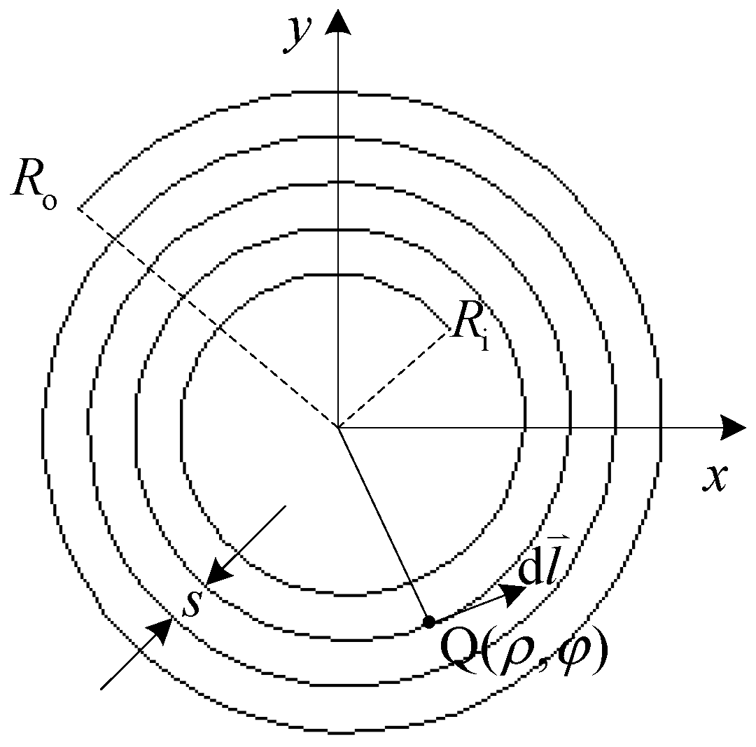
In the traditional method, each planar spiral coil is approximate to a cluster of series-connected concentric circular coils. If the inner and outer radii of a spiral coil are
Ri and
Ro, respectively, there are
N turns in the approximate cluster of concentric circular coils, so the radius of the innermost turn is
Ri =
Ro − (
N − 1)
s, and the radius of the
jth turn is
Ri + (
j − 1)
s,
j = 1,2,…,
N [
14]. In this way, a couple of spiral coils as shown in
Figure 2 is approximate to two clusters of concentric circular loops, and their number of turns are
N1 and
N2, respectively. The mutual inductance between such a couple of coils can be expressed as [
2,
14]:
where
i and
j represent the
ith and
jth turn of the two coils, respectively.
Mij is the mutual inductance between the
ith approximate circular loop of C
1 (radius
R1i) and the
jth approximate circular loop of C
2 (radius
R2j).
Mij is calculated by Maxwell’s formula [
6]:
where
,
K(
m), and
E(
m) are complete elliptic integrals of the first and second kind [
7]. The complete elliptic integral in (9) is approximated by the series expansion method.
2.2.3. Verification of the Method Proposed in This Paper and Its Comparison with the Traditional Methods
Equation (7) is an exact expression expressed by a double integral, which is concise in form and convenient to use. However, the traditional method is an approximation approach, which needs to calculate the radius of each circle of these two clusters of concentric coils, then through series expansion calculation and finally double summation, mutual inductance can be obtained.
The calculation results of Equation (7) are verified by the 3D finite element method (FEM). Their differences with the traditional method can be compared through the specific examples below, and the influences of coil parameters on mutual inductance can be studied. For a couple of coaxial spiral coils with five turns each, the solution type of the 3D FEM model is chosen as “Magnetostatic”, the current is uniformly distributed on the coil’s cross section, the mesh is assigned as “length based”, and the maximum length of elements is set as the default value.
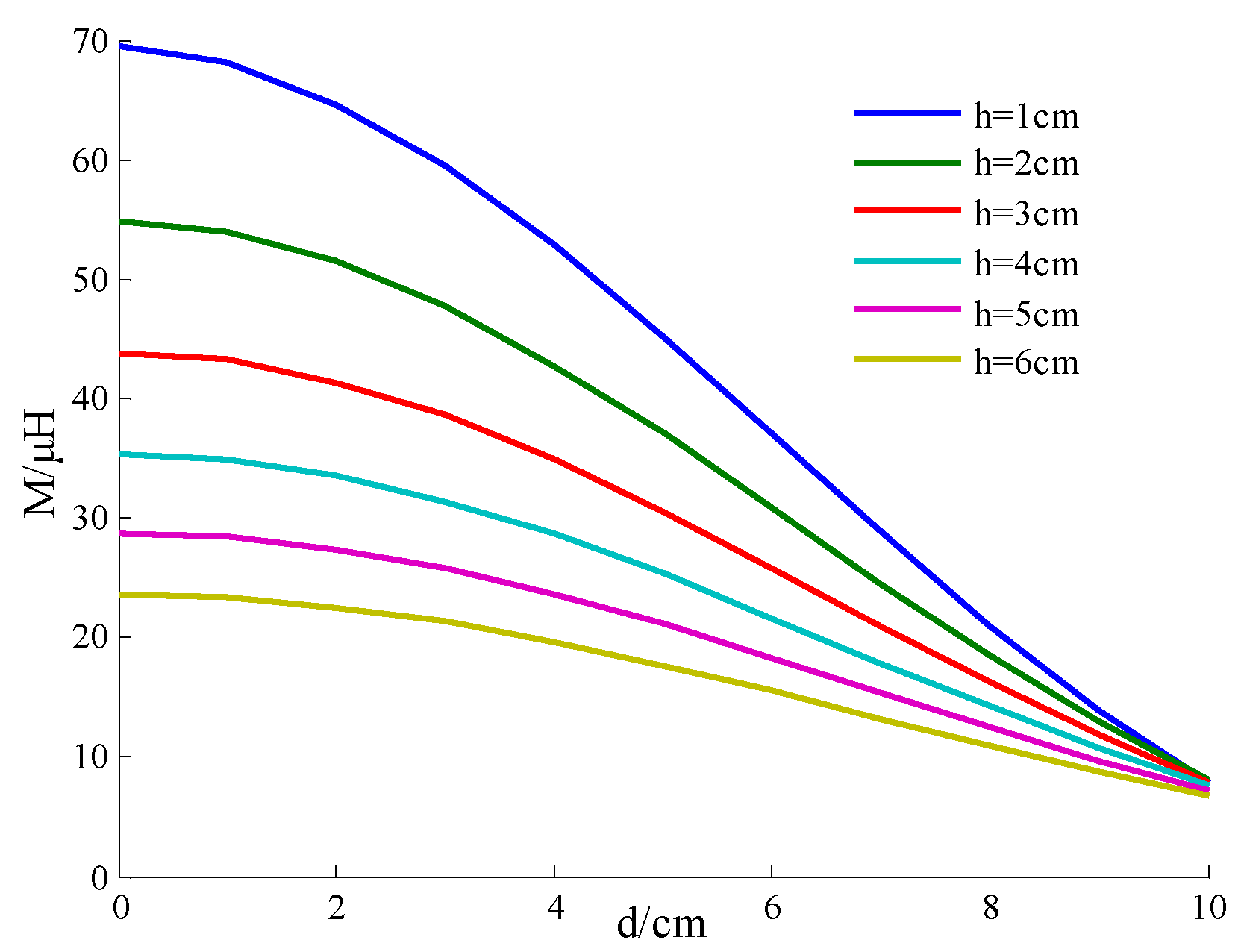
(a) Variation of the distance
Table 1 shows the mutual inductance calculation results at three different distances for a couple of coaxial spiral coils with outer radii
Ro1 =
Ro2 = 0.1 m and screw pitches
s1 =
s2 = 0.01 m.
M3D stands for 3D FEM results;
MS represents the results of Equation (7) and
ES represents their errors relative to
M3D;
MT represents the results of the traditional circular coils approximation method and
ET represents their errors relative to
M3D.
(b) Variation of the screw pitches
Table 2 shows the mutual inductance calculation results at three different screw pitches for a couple of coaxial spiral coils with
Ro1 =
Ro2 = 0.1 m and distances
h = 0.02 m.
(c) Variation of the external radius
Table 3 shows mutual inductance calculation results at three different outer radii for a couple of coaxial spiral coils with
h = 0.02 m and
s1 =
s2 = 0.01 m.
(a) The calculation results of Equation (7) in this paper are close to that from Maxwell 3D with little difference. The test shows that the larger the 3D region of the simulation setting is, the smaller the differences are, but the simulation time will be longer.
(b) The relative errors between the traditional circular coils approximation method and the 3D FEM results are obvious. For the traditional method, the error increases with distances when outer radii and screw pitches are fixed; the error increases with screw pitches when outer radii and distances are fixed; the error decreases with outer radii when distances and screw pitches are fixed.
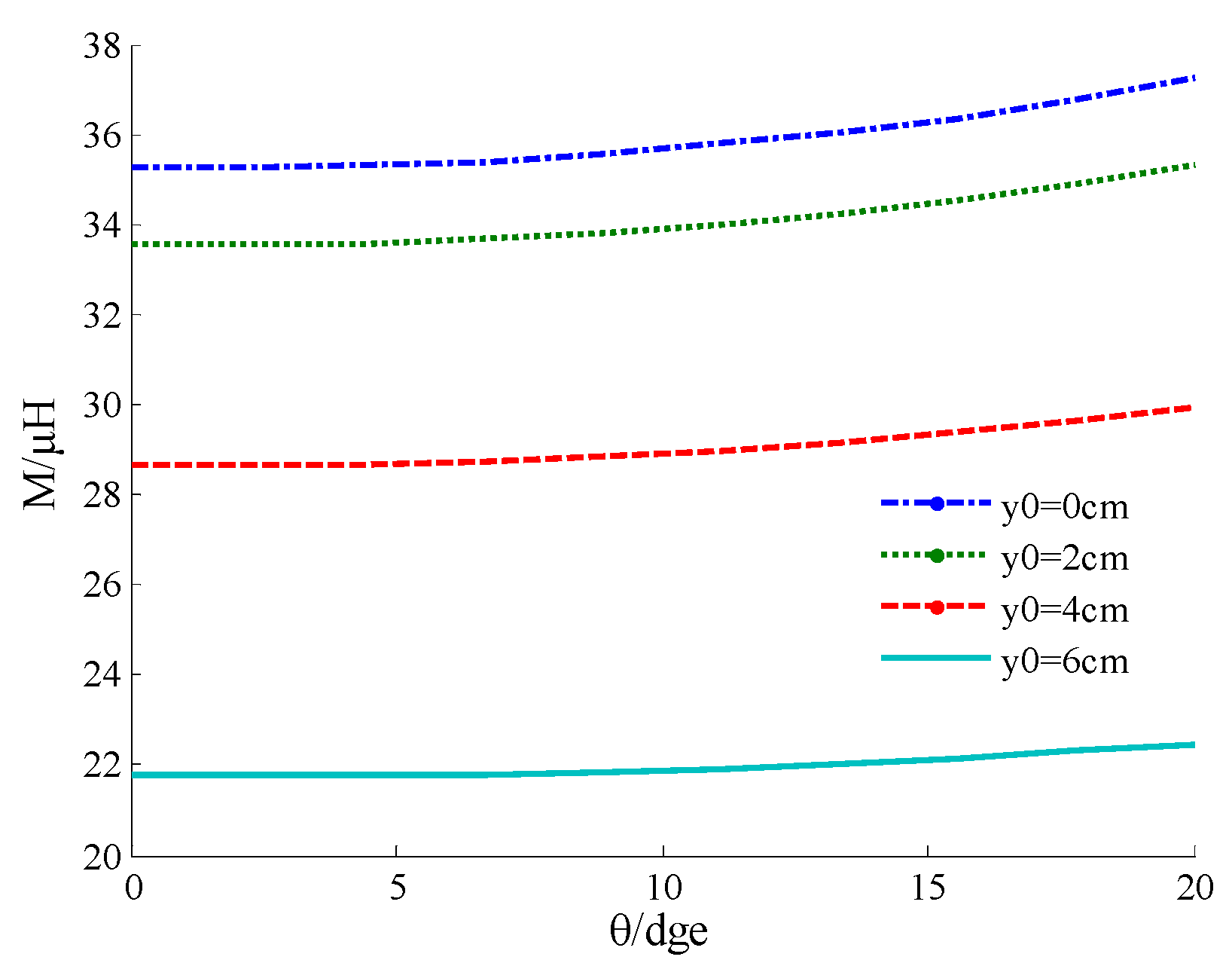
(c) The mutual inductance decreases with distances at fixed outer radii and screw pitches, decreases with screw pitches at fixed outer radii and distances, and increases with outer radii at fixed distances and screw pitches.
In terms of computational efficiency, for the above example, the calculation time of the proposed method is in the level of 10−1 s, while the traditional method is in the level of 10−2 s. However, it takes more than 10 h to simulate a 3D model established by ANSYS Maxwell considering the helicity.


