Numerical Modeling of Space–Time Characteristics of Plasma Initialization in a Secondary Arc

Abstract
:1. Introduction
2. Model Description
2.1. Governing Equations
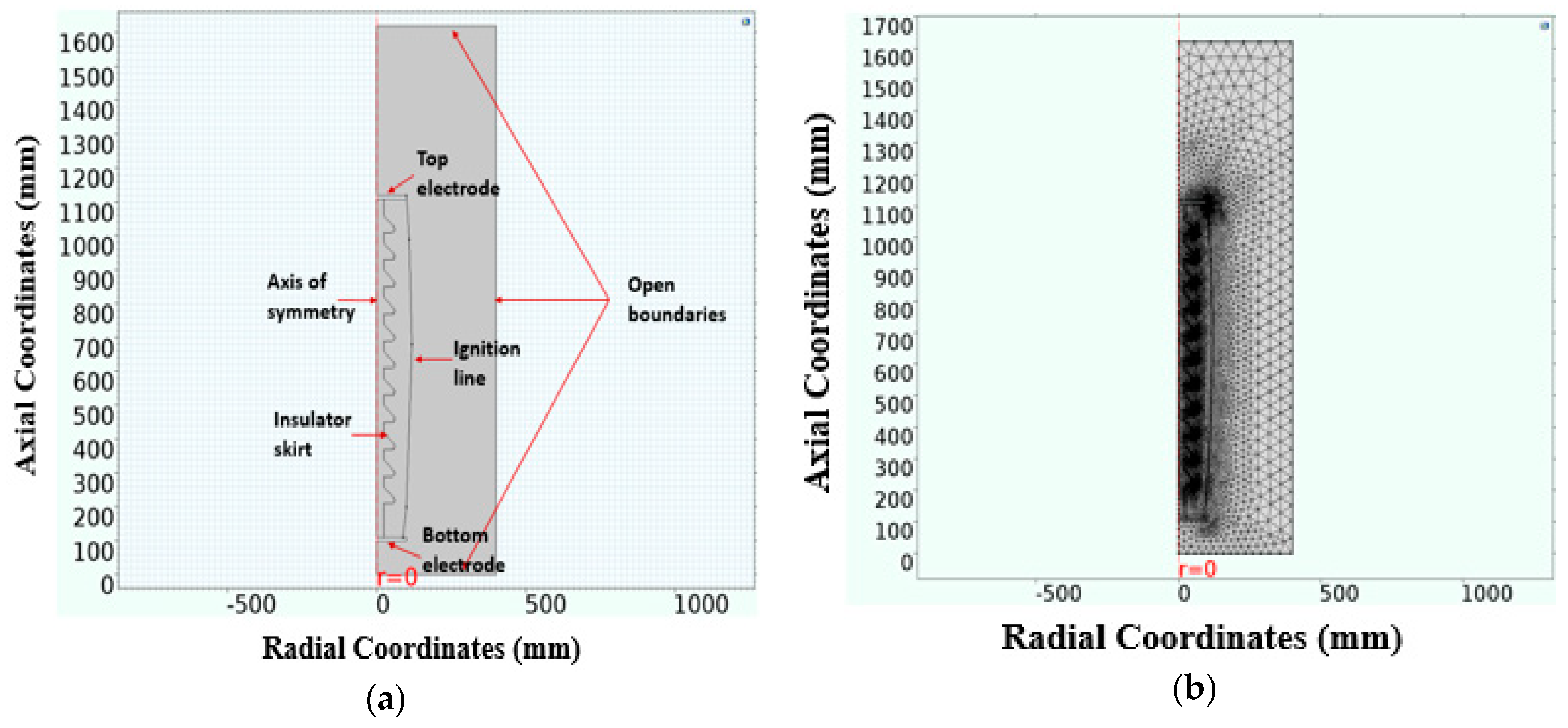
2.2. Computational Domain and Meshing
2.3. Numerical Modelling of the Short-Circuit Arc
2.4. Boundary and Initial Conditions
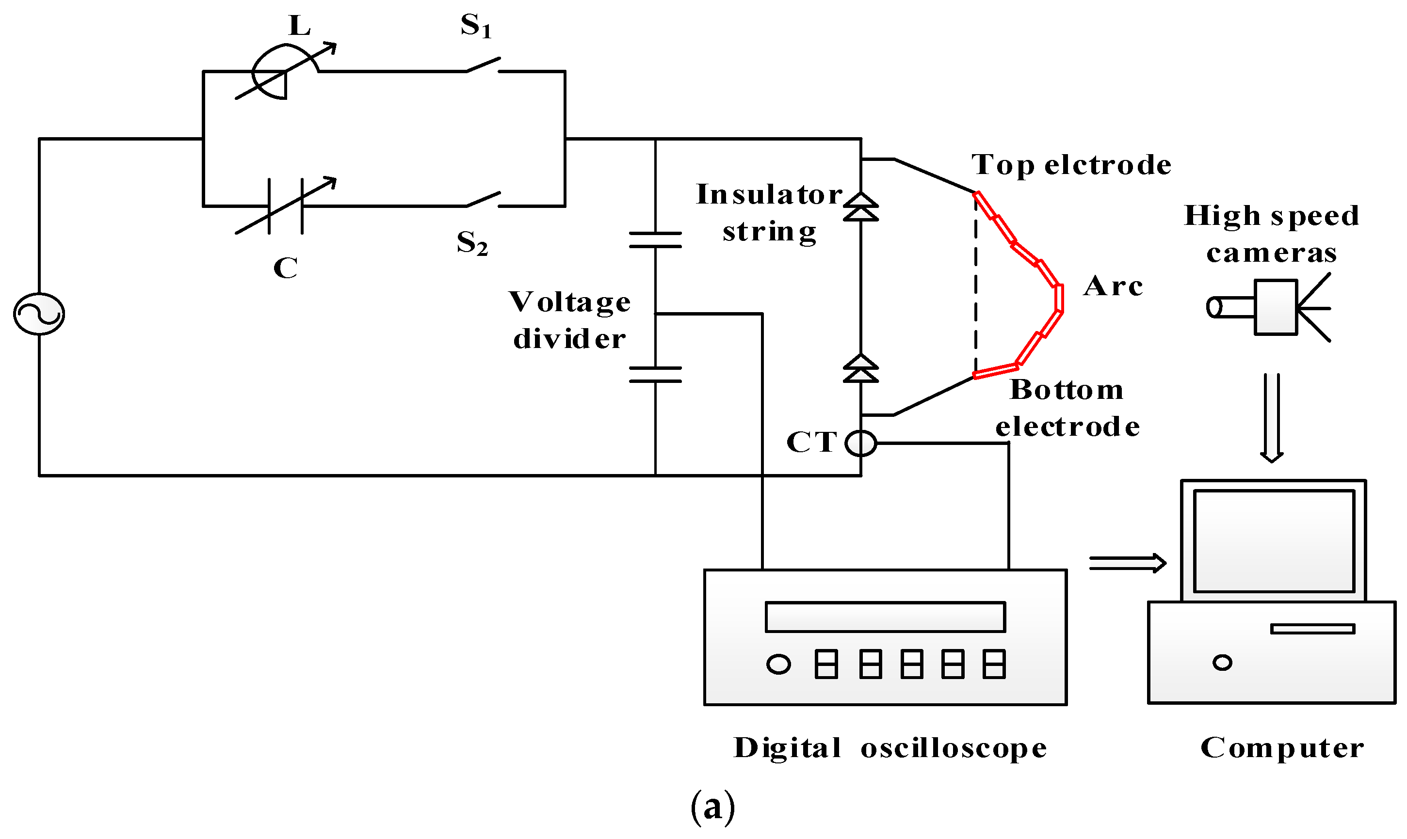
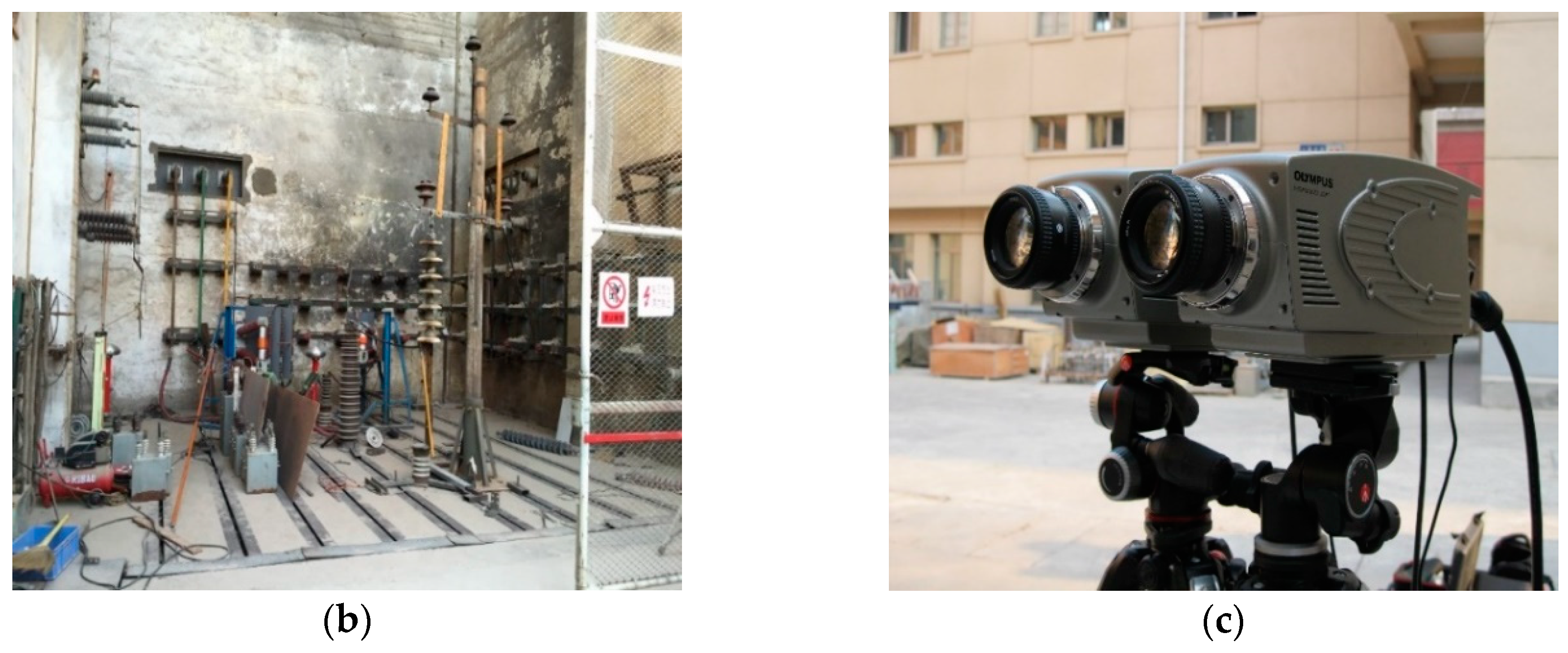
2.5. Experimental Platform
3. Results and Discussion
3.1. Experiment Verification
3.2. Particle Density Distribution and Development Law
3.3. Spatial Distribution of the Electric Field During Discharge
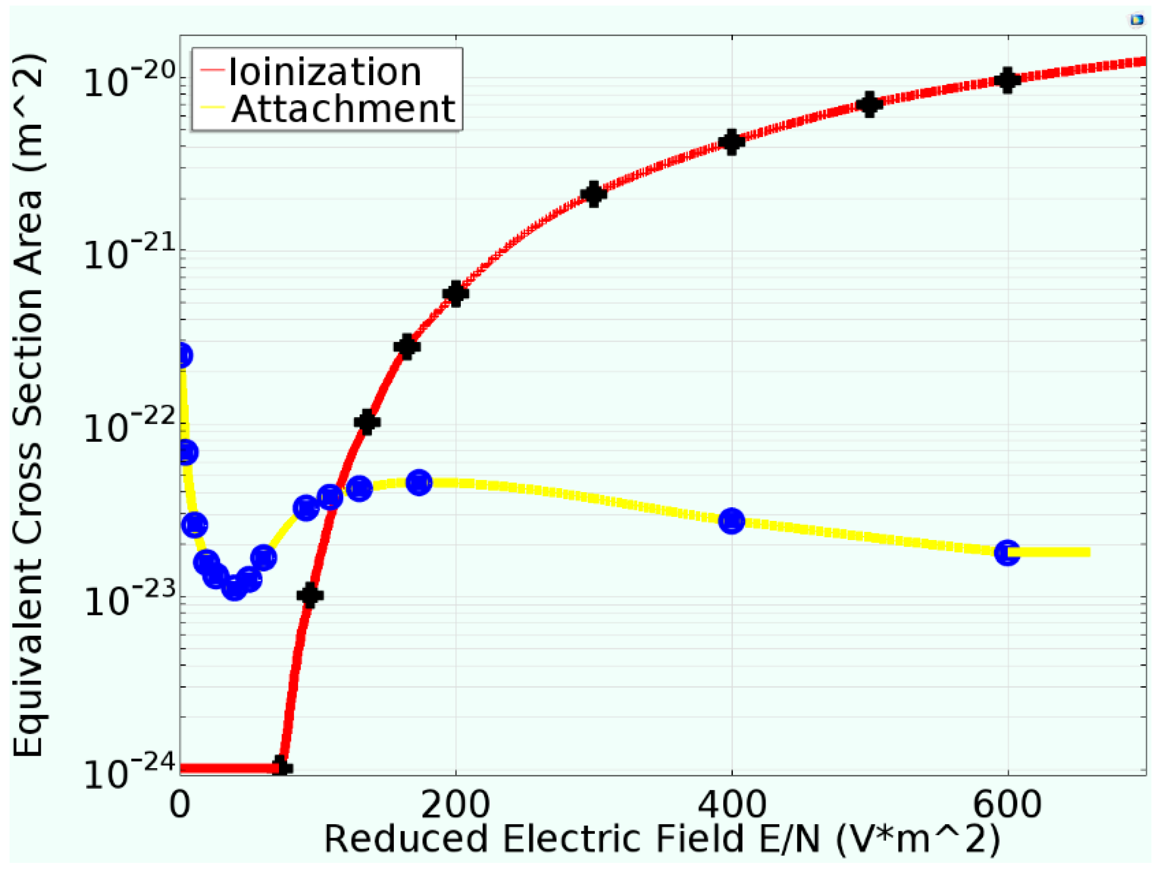
3.4. Particle Reactions in Discharge Process
4. Conclusions
- (1)
- The brightness distribution obtained by high-speed cameras of the experimental short-circuit arc was basically consistent with the predicted distribution of electron density, demonstrating that the simulation was effective and supported the subsequent analysis of the plasma interior.
- (2)
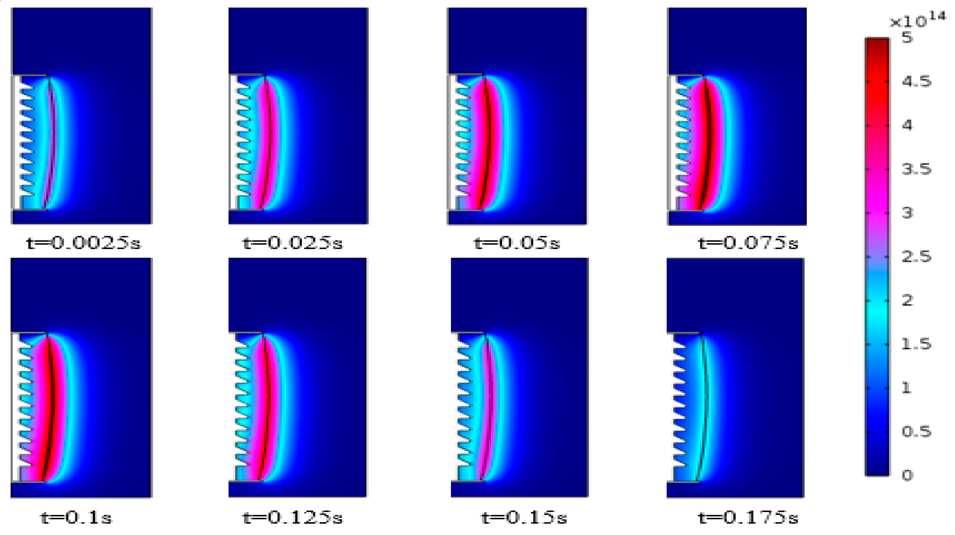
- With the short-circuit discharge, the electron density along the ignition line first increased and then decreased, and its distribution was quite different from the general streamer discharge. Over time, the concentration of negative ions rose and then levelled off, and due to the differences of diffusion, convection, and adsorption coefficients between positive ions and negative ions, the changing curves of concentrations of positive ions and negative ions had slight differences despite showing the same trend. Near the end of the simulation time, there was a considerably larger number of charged particles than the initial level, which provided the necessary environmental conditions for subsequent secondary arc generation.
- (3)
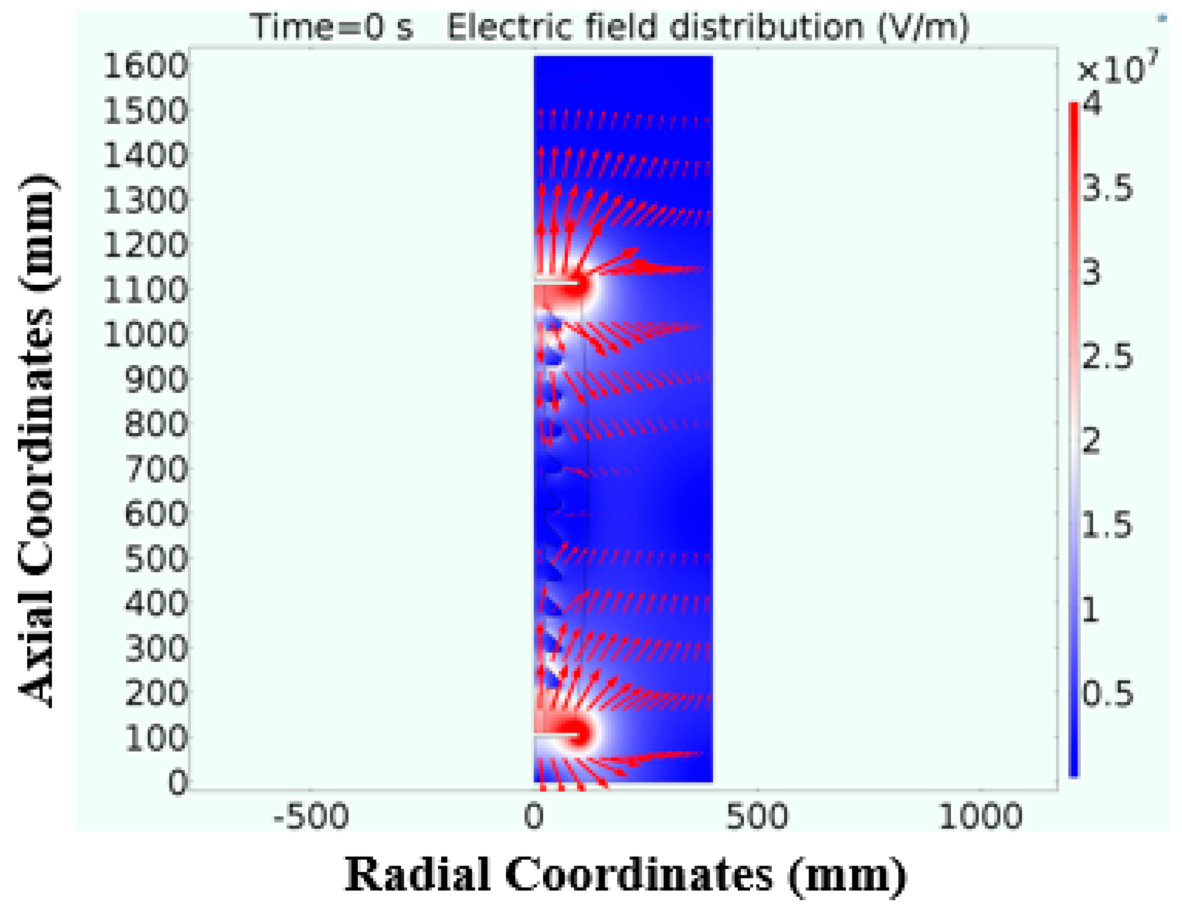
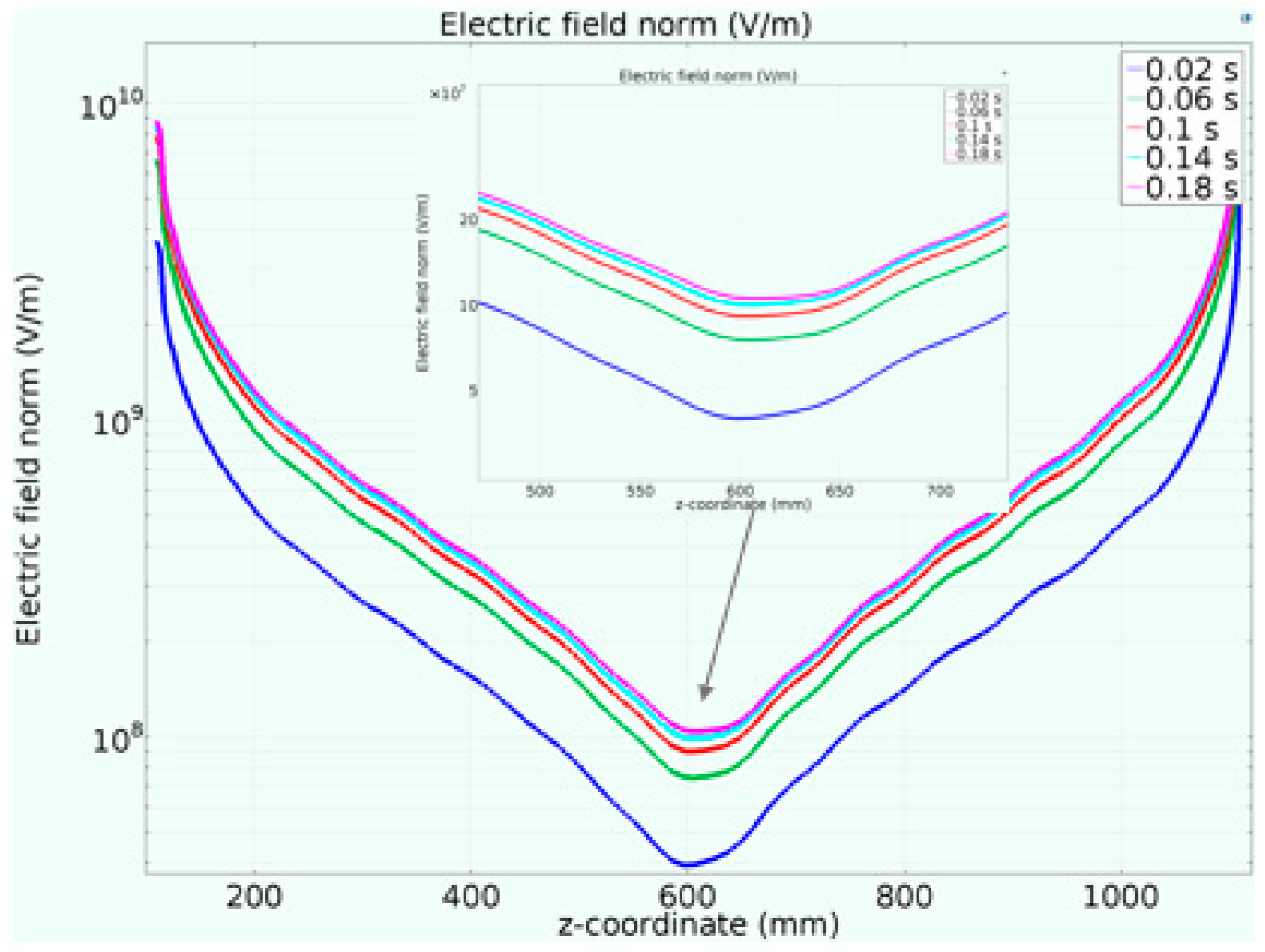
- The initial stage of discharge was mainly point discharge in space. The spatial electric field intensity showed an S-shaped upward trend in the discharge process. The end regions were Sssignificantly affected by the high-voltage electrode, whereas the middle area was mainly affected by the particle reaction.
- (4)
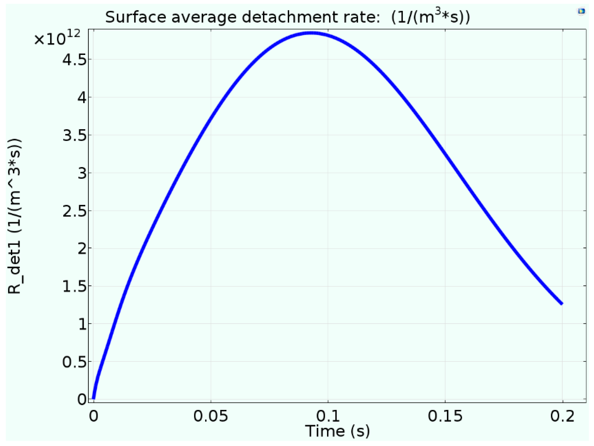
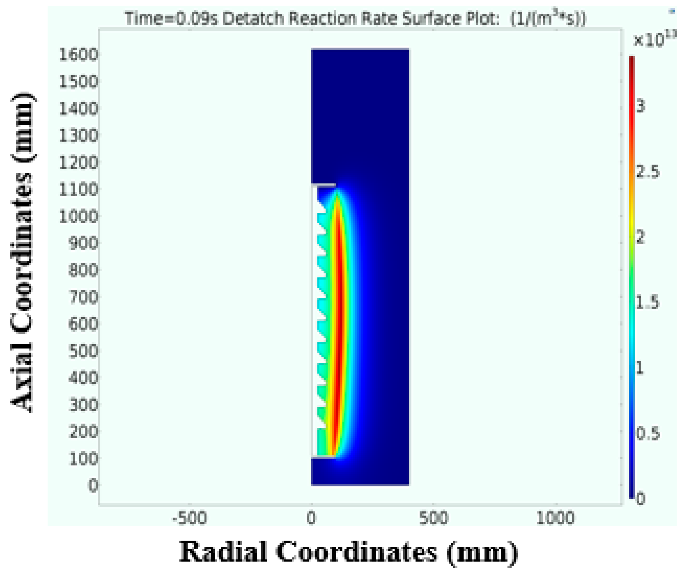
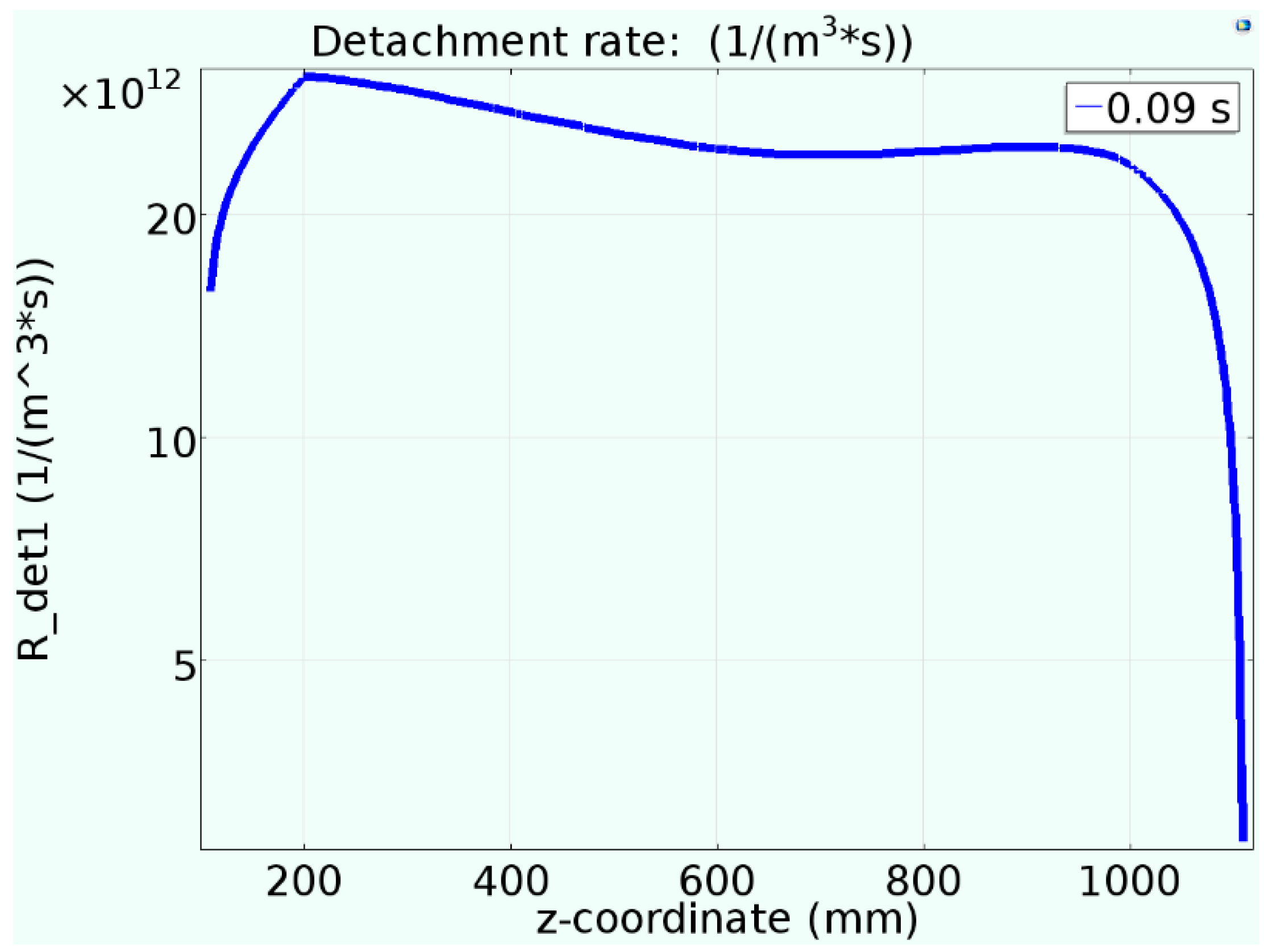
- The time correspondence between the detachment reaction and the ion source generated in the short-circuit discharge process was basically consistent, and the detachment reactions were mainly concentrated in the middle area and near the negative electrode. The average recombination reaction rates were consistent with the trend of the detachment reaction rate during the discharge, with differences only in magnitude.
Author Contributions
Funding
Conflicts of Interest
References
- Esztergalyos, J.; Andrichak, J.; Colwell, D.H.; Dawson, D.C.; Jodice, J.A.; Murray, T.J.; Nail, G.R.; Politis, A.; Pope, J.W.; Rockefeller, G.D.; et al. Single-phase tripping and auto reclosing of transmission lines. IEEE Trans. Power Deliv. 1992, 7, 182–192. [Google Scholar]
- Prikler, L.; Kizilcay, M.; Bán, G.; Handl, P. Modeling secondary arc based on identification of arc parameters from staged fault test records. Int. J. Electr. Power 2003, 25, 581–589. [Google Scholar] [CrossRef]
- Cong, H.; Du, S.; Shu, X.; Li, Q. Research portfolio and prospect on physical characteristics and modelling methods of secondary arcs related to high-voltage power transmission lines. Int. J. Appl. Electromagn. 2018, 56, 195–209. [Google Scholar] [CrossRef]
- Tsuboi, T.; Takami, J.; Okabe, S.; Aoki, K.; Yamagata, Y. Study on a field data of secondary arc extinction time for large-sized transmission lines. IEEE Trans. Dielectr. Electr. Insul. 2013, 20, 2277–2286. [Google Scholar] [CrossRef]
- Tavares, M.C.; Talaisys, J.; Camara, A. Voltage harmonic content of long artificially generated electrical arc in out-door experiment at 500 kV towers. IEEE Trans. Dielectr. Electr. Insul. 2014, 29, 1005–1014. [Google Scholar] [CrossRef]
- Li, Q.; Cong, H.; Sun, Q.; Xing, J.; Chen, Q. Characteristics of secondary ac arc column motion near power transmission line insulator atring. IEEE Trans. Power Deliv. 2014, 29, 2324–2331. [Google Scholar] [CrossRef]
- Gu, S.; He, J.; Zeng, R.; Zhang, B.; Xu, G. Motion characteristics of long ac arcs in atmospheric air. Appl. Phys. Lett. 2007, 90, 051501. [Google Scholar] [CrossRef]
- Terzija, V.V.; Wehrmann, S. Long arc in still air: Testing, modelling and simulation. EEUG News 2001, 7, 44–54. [Google Scholar]
- Johns, A.T.; Aggarwal, R.K.; Song, Y.H. Improved techniques for modeling fault arcs on faulted EHV tranmission system. IET Proc. Gener. Transmis. Distrib. 1994, 141, 148–154. [Google Scholar] [CrossRef]
- Kizilcay, M. Evaluation of existing secondary arc models. EEUG News 1997, 3, 49–60. [Google Scholar]
- Gu, S.; He, J.; Zhang, B.; Xu, G.; Han, S. Movement simulation of long electric arc along the surface of insulator string in free air. IEEE Trans. Magn. 2006, 42, 1359–1362. [Google Scholar]
- Horinouchi, K.; Nakayama, Y.; Hidaka, M.; Yonezawa, T.; Sasao, H. A method of simulating magnetically driven arcs. IEEE Trans. Power Deliv. 1997, 12, 213–218. [Google Scholar] [CrossRef]
- Cong, H.; Li, Q.; Xing, J.; Siew, W.H. Modeling study of the secondary arc with stochastic initial positions caused by the primary arc. IEEE Trans. Plasma Sci. 2015, 43, 2046–2053. [Google Scholar] [CrossRef]
- Sima, W.; Tan, W.; Yang, Q.; Luo, B.; Li, L. Long AC Arc movement model for parallel gap lightning protection device with consideration of thermal buoyancy and magnetic force. Proc. CSEE 2011, 31, 138–145. [Google Scholar]
- Birdsall, C.K.; Langdon, A.B. Plasma Physics via Computer Simulation; CRC Press: Boca Raton, FL, USA, 1991. [Google Scholar]
- Shi, J.; Kong, M. Cathode fall characteristics in a DC atmospheric pressure glow discharge. J. Appl. Phys. 2003, 94, 5504–5513. [Google Scholar] [CrossRef]
- Bogaerts, A.; Gijbels, R. Numerical modeling of gas discharge plasmas for various applications. Vacuum 2003, 69, 37–52. [Google Scholar] [CrossRef]
- Davies, A.J.; Davies, C.S.; Evans, C.J. Computer simulation of rapidly developing gaseous discharges. Proc. IEE Sci. Meas. Technol. 1971, 118, 816–823. [Google Scholar] [CrossRef]
- Singh, S.; Serdyuk, Y.; Summer, R. Adaptive numerical simulation of streamer propagation in atmospheric air. In Proceedings of the COMSOL Conference, Rotterdam, The Netherlands, 23–25 October 2013. [Google Scholar]
- Singh, S. Computational Framework for Studying Charge Transport in High-Voltage Gas-Insulated Systems; Chalmers University of Technology: Gothenburg, Sweden, 2017; pp. 14–17. [Google Scholar]
- Georghiou, G.E.; Papadakis, A.P.; Morrow, R.; Metaxas, A.C. Numerical modelling of atmospheric pressure gas discharges leading to plasma production. J. Phys. D Appl. Phys. 2005, 38, R303–R328. [Google Scholar] [CrossRef]
- Cong, H.; Li, Q.; Du, S.; Lu, Y.; Li, J. Space Plasma Distribution Effect of Short-Circuit Arc on Generation of Secondary Arc. Energies 2018, 11, 828. [Google Scholar] [CrossRef]
- Tran, T.N.; Golosnoy, I.O.; Lewin, P.L.; Georghiou, G.E. Numerical modelling of negative discharges in air with experimental validation. J. Phys. D Appl. Phys. 2011, 015203. [Google Scholar] [CrossRef]
- Cong, H.; Li, Q.; Xing, J.; Li, J.; Chen, Q. Critical length criterion and the arc chain model for calculating the arcing time of the secondary arc related to AC transmission lines. Plasma Sci. Technol. 2015, 17, 475. [Google Scholar] [CrossRef]


| Transport Parameters | Expression | Description |
|---|---|---|
| (m2/Vs) | 2.0 × 10⁻⁶ | Positive ion mobility |
| (m2/s) | 5.05 | Positive ion diffusivity |
| (m2/Vs) | 2.2 × 10⁻⁶ | Negative ion mobility |
| (m2/s) | 5.56 | Negative ion diffusivity |
| (m3/s) | 5.0 × 10⁻¹⁴ | Electron-positive ions recombination rate |
| (m3/s) | 2.07 × 10⁻¹³ | Positive-negative ions recombination rate |
| f0 (1/m3s) | 1.7 × 10⁹ | Natural background ionization source item |
| kdet (m3/s) | 1 × 10⁻¹⁸ | Electron detachment coefficient from negative ions |
| Application Location | Convection and Diffusion | Convection and Diffusion | Convection and Diffusion |
|---|---|---|---|
| Axis of symmetry | |||
| Top electrode | |||
| Bottom electrode | |||
| Ignition line | |||
| Rest of the boundary |
© 2019 by the authors. Licensee MDPI, Basel, Switzerland. This article is an open access article distributed under the terms and conditions of the Creative Commons Attribution (CC BY) license (http://creativecommons.org/licenses/by/4.0/).
Share and Cite
Li, J.; Yu, H.; Jiang, M.; Liu, H.; Li, G. Numerical Modeling of Space–Time Characteristics of Plasma Initialization in a Secondary Arc. Energies 2019, 12, 2128. https://doi.org/10.3390/en12112128
Li J, Yu H, Jiang M, Liu H, Li G. Numerical Modeling of Space–Time Characteristics of Plasma Initialization in a Secondary Arc. Energies. 2019; 12(11):2128. https://doi.org/10.3390/en12112128
Chicago/Turabian StyleLi, Jinsong, Hua Yu, Min Jiang, Hong Liu, and Guanliang Li. 2019. "Numerical Modeling of Space–Time Characteristics of Plasma Initialization in a Secondary Arc" Energies 12, no. 11: 2128. https://doi.org/10.3390/en12112128