Abstract
The ice coating on the transmission line is extremely destructive to the safe operation of the power grid. Under natural conditions, the thickness of ice coating on the transmission line shows a nonlinear growth trend and many influencing factors increase the difficulty of forecasting. Therefore, a hybrid model was proposed in this paper, which mixed Ensemble Empirical Mode Decomposition (EEMD), Random Forest (RF) and Chaotic Grey Wolf Optimization-Extreme Learning Machine (CGWO-ELM) algorithms to predict short-term ice thickness. Firstly, the Ensemble Profit Mode Decomposition model was introduced to decompose the original ice thickness data into components representing different wave characteristics and to eliminate irregular components. In order to verify the accuracy of the model, two transmission lines in ‘hunan’ province were selected for case study. Then the reserved components were modeled one by one, building the random forest feature selection algorithm and Partial Autocorrelation Function (PACF) to extract the feature input of the model. At last, a component prediction model of ice thickness based on feature selection and CGWO-ELM was established for prediction. Simulation results show that the model proposed in this paper not only has good prediction performance, but also can greatly improve the accuracy of ice thickness prediction by selecting input terminal according to RF characteristics.
1. Introduction
Since the 21st century, due to the increasing demand for electricity caused by the rapid development of the national economy, power grid construction of China has entered a period of rapid development. The natural environment of different regions in China is quite different, which increases the probability of transmission lines suffering meteorological disasters and affects the safe and stable operation of transmission lines [1]. For transmission lines, icing hazard is one of the most common and serious hazards, posing a huge threat to the safety and stability of the lines [2]. Hence, it is convenient to predict the thickness of line icing to carry out timely response to the damage caused by icing, so as to ensure the safe and stable operation of power grid.
For the model of line icing prediction, domestic scholars have done a lot of research, mainly divided into two methods. One is to use the physical model to predict the growth of the shape, density, and weight of the icing on the wire. The analysis and research models are noted as the Makkonen model, Imai model, Goodwin model, etc. [3,4]. However, as important as parameters in the model, which are difficult to collect, the prediction effect of the physical model is poor. The other is based on factors affecting the ice sheet and its development, and intelligent algorithms are used to predict the ice sheet thickness data fit. Lan, D.L and Zheng, Z.H used Generalized Regression Neural Network (GRNN) method to forecast ice thickness, with the results suggesting that the GRNN method shows good performance in ice coating thickness [5]. Xiao-min ma proposed a forecasting model based on grey Support Vector Machine (SVM) short-term ice thickness of transmission line [6], and the results showed that the SVM method can accurately predict the short-term ice thickness. However, GRNN and SVM methods all have systematic errors in simulation. The GRNN model relies too much on the sample data. When the sample data set is not sufficient, the GRNN neural network may lead to poor adaptability; for the SVM method, the kernel function and kernel parameters affect the fitting accuracy and generalization ability to varying degrees.
Due to the faster convergence speed and less human interference compared with the traditional neural network, the Extreme Learning Machine (ELM) proposed by huang in 2004 has been widely used in many prediction fields. Zhang ning, huang yuanyu, li wanhua et al. [7,8,9] used the ELM model to predict short-term load based on various influencing factors, whose results showed that compared with the traditional Back Propagation (BP) neural network model, the ELM model could be better and more effective in short-term load prediction. Zhong Wang, Jilao Chen et al. [10,11] by decomposing wind speed data, used the inherent model components of the decomposed data in the ELM model for forecasting. Jian-li liu [12] and others used the Particle Swarm Optimization (PSO) method, and found a set of optimal ELM mapping parameters, in order to improve the ability of dealing with linear inseparable problem, with the results showing that this algorithm has higher accuracy; Lai min [13] made use of sine Chaotic Adaptive Whale Optimization Algorithm (CAWOA) to search and optimize the model parameters of the extreme learning machine in order to improve the generalization ability of ELM, whose results show that CAWOA-ELM has better generalization ability and can predict NO2 emissions more accurately. To sum up, it can be found that the ELM prediction model has been able to predict successfully in different fields. However, the input weight matrix of randomly assigned ELM and the deviation of hidden layer may affect the generalization ability of ELM, which represents that it is necessary to use the optimization algorithm to obtain the optimal weight of input layers and the deviation of hidden layers. A new algorithm (Gray Wolf Optimization algorithm (GWO)) first proposed by Mirjalili et al. due to its low complexity, low control parameters, strong search capability, and high efficiency, is widely used in function optimization and other problems. Tan nian et al. proposed a prediction model of wood density based on GWO-SVM, which used near infrared spectroscopy (NIR) to predict the density of Chinese fir. The results show that the Grey Wolf algorithm is reasonable and efficient to predict the density of Chinese fir with SVM and NIR [14]. Yang proposed a BP neural network image restoration algorithm optimized by Gray Wolf algorithm, whose results showed that the algorithm had faster convergence speed and higher restoration accuracy than the Genetic Algorithm-Back Propagation (GA-BP) algorithm [15].
Considering the high complexity and volatility of the icing thickness, most historical literature directly model and predict the icing thickness, so the effect is not ideal. Therefore, this paper uses Ensemble Empirical Mode Decomposition (EEMD) method for the first time to decompose the icing thickness, which effectively solves the problem of mode aliasing, retains the real signal to the maximum extent, builds the prediction model based on the decomposition of the original signal, and can effectively improve the accuracy [16,17,18,19,20,21,22].
From another perspective, as transmission line icing thickness is a time series change, two prediction methods were proposed to predict accuracy icing thickness data. One is based on historical data of icing thickness, but as the phenomenon of ice coating on the transmission line is a physical phenomenon determined by various factors, the prediction of this method is not accurate. For great accuracy, the second prediction method comes into being, which is based on the analysis of the influencing factors of line icing thickness. Moster [23] et al. predicted the ultra-short-term liquid water content, wind speed, and rainfall in the air based on the grey correlation system theory, and calculated the ice cover growth rate. The results showed that the prediction accuracy could be better improved through factor analysis. At present, most of the influencing factors are selected through the Grey Relation Analysis (GRA), but several influencing factors may influence each other. Under these circumstances, this paper proposes to use the random forest intelligence algorithm for the first time, which is a method for classification and regression, to select important influencing factors as the input variables for prediction by calculating the importance of computing features. Combining RF characteristics to improve the prediction accuracy of icing thickness is a novel direction in this paper [24,25,26].
In summary, this paper proposes a prediction model of icing thickness based on Ensemble Empirical Mode Decomposition (EEMD), Random Forest (RF), Chaotic Grey Wolf Algorithm (CGWO) and Extreme Learning Machine (ELM). Firstly, EEMD is introduced to decompose the historical ice-cover thickness series into multiple sub-sequences with different frequency fluctuation characteristics and reconstruct them according to the signal frequency; then, RF is applied to select the input variable of icing thickness for the reconstructed signals respectively, and the best model input variable set is selected for multiple variables with different lag periods; finally, a Chaotic Grey Wolf Algorithm-Extreme Learning Machine (CGWO-ELM) model is established for prediction and the prediction results of each reconstructed signal are added to obtain the final prediction results.
To sum up, the innovation and contribution of this research mainly focus on the following aspects:
- (1)
- The data of ice thickness with nonlinearity and instability, the EEMD model was applied to decompose the signal for the first time, and the original signal was divided into low-frequency signal, medium-frequency signal, and high-frequency signal.
- (2)
- The importance analysis by the RF algorithm for influencing factors was first proposed and applied to the field of icing thickness prediction. This paper systematically analyzes the factors affecting the thickness of icing and improves the accuracy of prediction.
- (3)
- Based on the GWO-ELM, this paper uses chaos algorithm to optimize the input weight and hidden deviation. The analysis and verification of the two lines with severe ice disasters show that the optimization can greatly improve the accuracy of the prediction.
For the convenience of readers, Table 1 shows the meaning of the symbols used in this article.

Table 1.
The meaning of the symbols used in this article.
2. Methodology
2.1. Ensemble Empirical Mode Decomposition (EEMD)
Empirical Mode Decomposition (EMD) was first proposed by Huang for signal analysis based on the adaptive data mining method. By decomposing the nonlinear sequence into a number of different Intrinsic Mode Functions (IMFs) components and a residual component (R), a stationary sequence is obtained, which is suitable for dealing with the ice thickness waveform with large volatility knots based on the signal’s own scale in the decomposition process [27]. In theory, EEMD can be applied to any type of time series signal, where the IMFs component needs to meet the following two conditions.
- (a)
- The number of zero crossings of the signal differs from the maximum number of local extremes by one.
- (b)
- The sequence means values within the entire domain range trend to zero.
The specific decomposition process of EMD is as follows:
- (1)
- Find all the extreme points (including the maximum value and the minimum value) in the original signal , and use the cubic spline difference function to fit the upper and lower envelopes of the original data.
- (2)
- Solve the median value of the upper and lower envelopes:
- (3)
- Let , if does not satisfy the two sufficient conditions of the IMF component, repeat steps (1) and (2) until h_k (t) satisfies these two conditions after i-iterations, we can get .
- (4)
- At this time, the IMF 1 is separated from the original signal, and the residual component is taken as the original signal. Then, the above steps are repeated, and the sequence signal is re-decomposed to obtain n-IMF components. When the residual component r(t) satisfies the monotonicity, the final result can be obtained.where is the IMF component and is the residual component.
However, the monitoring and acquisition of icing signal data often causes signal interruption, noise, and abnormality of the device caused by abnormal noise. In the process of modal decomposition, it will lead to erroneous IMF components, and it is prone to modal aliasing which cannot achieve better results. In order to solve the above problems, the EEMD method is proposed in this paper, and the process is as follows [28]:
- (1)
- First, a white noise sequence obeying the positive distribution is added to the original icing thickness signal to form a new target sequence.
- (2)
- The n-IMF components and a residual component can be found by EMD based on the new target sequence.
- (3)
- Steps (1) and (2) are iteratively iterated r times, with each iteration adopting a white noise sequence of different amplitudes, and finally the IMF component of r times is averaged as a whole, as the IMF component of the original time series signal.
2.2. Chaotic Grey Wolf Algorithm (CGWO)
As a subset of evolutionary computation, the Grey Wolf Optimization Algorithm (GWO), which was inspired by the wisdom behavior of the wolf group living in the Eurasian continent, was first proposed by the Mirjalili and other scholars in 2014 [29]. It has been shown that GWO with low complexity, few control parameters, high search efficiency, and higher efficiency than other optimization algorithms is widely used in function optimization.
In the GWO, α is set as the optimal solution, and β and δ are set as the second and third optimal solutions, ω is taken as remaining solution, at the same time, the hunting behavior is led by α, followed by three wolves: β, δ and ω, as shown in Figure 1 [30].
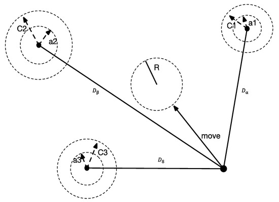
Figure 1.
The movement of the wolves.
In this paper, we introduced the chaos operator into the optimization algorithm to improve the algorithm and improve the global search ability of the algorithm. In particular, chaotic algorithms, which have the advantages of being generally universal, robust, and prevent the algorithm from falling into local optimum, can overcome the shortcomings of the random distribution of the initial population of GWO algorithm we called CGWO, make it evenly distributed, and improve the ubiquity of the population [31].
2.3. Extreme Learning Machine (ELM)
As a new single hidden layer forward neural network learning algorithm, extreme learning machine (ELM) is different from traditional neural network training learning in that the ELM hidden layer does not need iteration, input weight, and the hidden layer node offset is randomly selected and will be minimal, the minimum training error is the target, and the hidden layer output weight is finally determined [32]. With the advantages of fast learning speed and good generalization performance compared with the traditional training method, ELM has attracted more attention from experts and scholars worldwide [33]. The neural network structure of ELM is shown in Figure 2. However, the ELM algorithm has the disadvantages of initial weight and excessive threshold [34]. To solve the above problems, this paper proposes CGWO method to optimize the initial parameters of the ELM model.
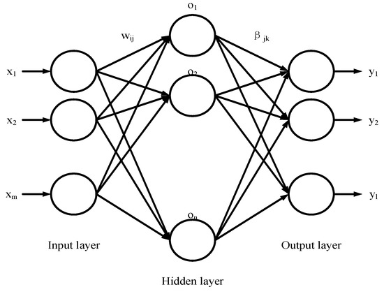
Figure 2.
Extreme Learning Machine (ELM) model structure.
2.4. Chaotic Grey Wolf Algorithm-Extreme Learning Machine (CGWO-ELM)
The input weight of the ELM and the threshold of the hidden layer are randomly given, and if the input weight and the hidden layer threshold are 0, some hidden layer nodes may be invalid. Therefore, in the actual application process, a large number of hidden layer nodes need to be set to meet the accuracy requirements. Meanwhile, because the initial weight and threshold of the ELM are randomly generated, a big gap between each training and learning result may be generated. In view of the above problems, this paper proposed a Chaos Grey Wolf Optimization-Extreme Learning Machine (CGWO-ELM) prediction algorithm. Specific steps are shown in Figure 3. Part 1 is the process of selecting the input of the prediction model by the grey correlation method. Part 2 is the optimization process of the CGWO method. Part 3 is the process of ELM prediction. The combined prediction model optimizes the weight and threshold of the ELM by the CGWO method.
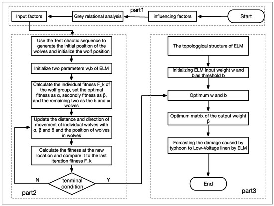
Figure 3.
Chaotic Grey Wolf Algorithm-Extreme Learning Machine (CGWO-ELM).
2.5. Random Forest (RF)
The random forest (RF) is based on the decision tree, and the random resampling technique and the node random splitting technique are used to extract samples from the original training set and establish a decision model. When Bootstrap sampling, about 36.8% of out-of-bag data will be generated each time, and the method of evaluating the performance of RF and decision tree prediction is using Out of Band (OOB). OOB as a test set is called OOB estimation [35]. Only if the number of trees in RF is sufficient, OOB is estimated to be unbiased.
For the RF that has been generated, the total number of OOB samples is set to , and when the OOB is used as the test set to verify the RF prediction performance, the correct number of samples tested is , the OOB prediction accuracy us and the calculation formula is as follows:
Feature importance metrics are an important feature of RF that can be used as feature selection tools for high-dimensional data. The main idea of Mean Decrease in Accuracy (MDA) is to determine the importance of the feature by permuting the influence of the characteristic variable on the prediction or classification result.
To set bootstrap samples (N is the number of training samples), they are characterized by (M is the number of feature dimensions). The variable importance measure based on OOB prediction accuracy is calculated as follows:
is the prediction accuracy obtained by adding noise to each feature and using OOB with noise as the test.
estimates the generalization error based on and based on this, the importance of the feature can be estimated. In RF, directly measures the influence of each feature on the accuracy of the model, sorts the importance of all features according to , and then selects those variables that are important to the model as the input of the model, thus achieving the purpose of feature selection [36].
2.6. Partial Auto Correlation Function (PACF)
In a system composed of multiple factors, when the influence or degree of correlation of one element on another is studied, the influence of other elements is regarded as a constant (maintained unchanged). In other words, the influence of other factors is not considered and the close relationship between the two elements is studied separately. By this way, the numerical result is the partial correlation coefficient.
is used to represent the j-th regression coefficient in the k-th order autoregressive equation, then the k-order autoregressive model is expressed as:
Here, k is the last coefficient. If it is regarded as a function of the lag period k, is called partial auto correlation function (PACF).
2.7. Model Building
The idea of the combined model built in this paper is shown in the Figure 4. First, the icing thickness data is decomposed by two methods. Then, the historical data selected by PACF and the more important influencing factors of RF selection are taken as the input, and the decomposed icing thickness data is used as the output of the prediction model. Finally, the icing thickness is predicted by different prediction models. The following is a detailed explanation of the combined model based on Figure 4.
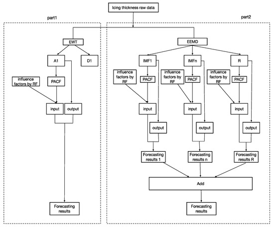
Figure 4.
The steps of icing thickness prediction.
In part 1, an approximate sequence A1 which will be used as forecast data and a high-frequency sequence D1, which will be ignored, are decomposed by the method of Empirical Wavelet Transform (EWT). Then the PACF is used to analyze the intrinsic relationship between the approximate series so as to select the inputs for CGWO-ELM with the influence factor selected by RF. The icing thickness data in the approximate series A1 is divided into a training set and a test set for prediction. Finally, the predictive results are compared with the actual icing thickness.
In the part 2, icing thickness is decomposed into several IMF values and a high stability residue R by the method EEMD. Similarly, PACF is used to analyze the correlation between each IMF, R, and the data to be predicted. The historical data with the highest correlation will be selected as the inputs of the CGWO-ELM model with the influence factor selected by the RF. Finally, the predicted data for the icing thickness will be composed of predicted values from all IMFs and R.
The establishment of the prediction model proposed in this paper firstly compares the decomposition methods that are more conducive to the icing thickness prediction model through two decomposition methods. Then, the selection of the influencing factors by RF and the historical data selection by PACF are made to determine the input end of the prediction model, which shows that the RF and PACF methods can show good performance in the prediction of icing thickness. Finally, the combined prediction method proposed in this paper predicts and adds the amount of decomposition to obtain the prediction result of the final icing thickness. In summary, this paper compares and analyzes the proposed prediction models to prove the accuracy, validity, and universality.
3. Empirical Analysis
3.1. Data Sources
The 2008 ice disaster in Hunan brought a serious power crisis to China, causing damage to a large number of transmission lines and collapse of towers. In the context of this typical event, this paper selected the “Yangdong Line” in Shaoyang, Hunan Province as a practical case to verify the accuracy of the methods presented in this article. From 8 January to 3 March 2008, a total of 440 sets of transmission line data were selected, which were provided by the Key Laboratory of Disaster Prevention and Mitigation of Power Transmission and Transformation Equipment (Changsha, China).
3.2. Icing Thickness Decomposition
In Figure 5, it is easy to see that icing thickness has the characteristics of irregularities, variability, and random fluctuations. As a result of this, the methods of EEMD and EWT were used to decompose the time series of icing thickness with the purpose of reducing noise interference. The result is shown in Figure 6, Figure 7 and Figure 8.
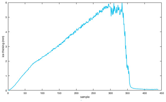
Figure 5.
Icing thickness change trend of “Yangdong Line.”
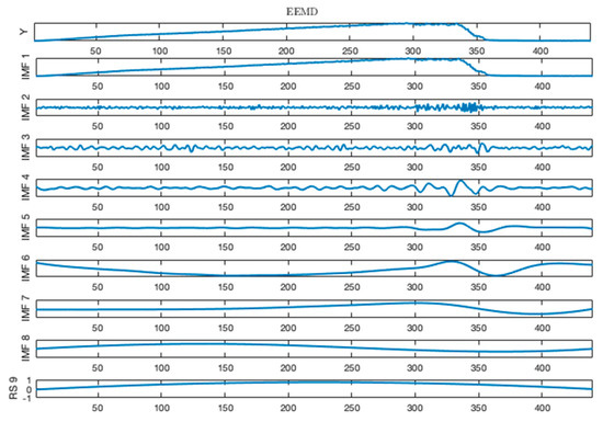
Figure 6.
Ensemble Empirical Mode Decomposition (EEMD) of “Yangdong Line.”
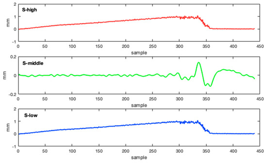
Figure 7.
Signal reconstruction of EEMD of “Yangdong Line.”
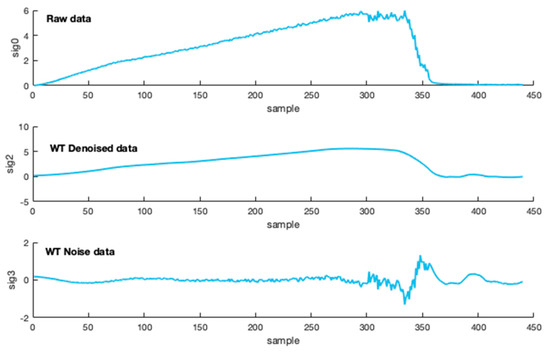
Figure 8.
EWT noise reduction of “Yangdong Line.”
Figure 6 shows the icing thickness in seven IMFs and one residual R by the EEMD with shorter running time. For the convenience of calculation, eight sub-signals were reconstructed according to the frequency. The eight sub-signals were divided into high-frequency signal class (IMF 1–3) called S-high, intermediate frequency signal class (IMF 4–5) called S-middle and low-frequency signal class (IMF 6-8, R) called S-low, according to the frequency level, as shown in Figure 7.
Figure 8 shows the icing thickness is divided into an approximate variable A1 which is considered as a smooth substitute for the raw data, as well as the predicted icing thickness and a detail variable D1 which is ignored as a high frequency sequence by the method of EWT.
In this paper, whether it is a batch of IMF decomposed by EEMD, or the A1 value obtained by noise reduction according to EWT, the first 340 sets of data were used as the training set, and the last 100 sets of data were used for testing.
3.3. Input Selection
This paper mainly analyzes the factors affecting the thickness of icing and the time series change for the prediction of icing thickness. In other words, the external weather factor and the trend of the icing thickness itself.
In order to make the prediction of icing thickness more accurate, the meteorological factors which are filtered and selected by random forest algorithm (RF) were used to select the main influencing factors as part of the prediction input.
Figure 9 and Figure 10 show the calculation of the importance of each feature input of the sub-signals generated by the two decomposition methods. From left to right the feature inputs are: Temperature (°C) recorded as “1,” Air humidity (%) recorded as “2,” Wind speed (m/s) recorded as “3,” Wind angle recorded as “4,” Light intensity (W/m2) recorded as “5,” Air pressure (Mpa) recorded as “6,” Freezing duration (t) recorded as “7,” Ice coverage uniformity recorded as “8,” Rain and snow duration (t) recorded as “9” [37]. Based on the ranking of characteristic importance, the more important influencing factors were selected as the feature inputs of the prediction model. Table 2 shows the input characteristics of the influencing factors.
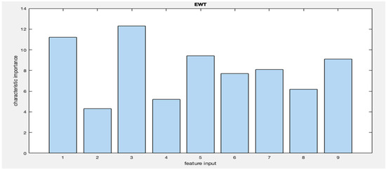
Figure 9.
Importance of A1 signal by EWT characteristic of “Yangdong Line.”
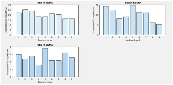
Figure 10.
Importance of high frequency, intermediate frequency, and low frequency signal by EEMD characteristic of “Yangdong Line.”
Table 2.
Input factors for random forest analysis selection of “Yangdong Line.”
In order to verify the correlation between the historical data of the icing thickness and the predicted data, this paper uses the PACF method which was used to find the Lags with significant elimination of internal characteristics to select another part of the input part of the prediction model. Figure 11 shows the PACF results for A1 decomposed by EWT. Figure 12 shows PACF results for reconstructed icing thickness signal by EEMD.
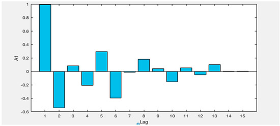
Figure 11.
The partial auto correlation function (PACF) results of A1 by EWT of “Yangdong Line.”
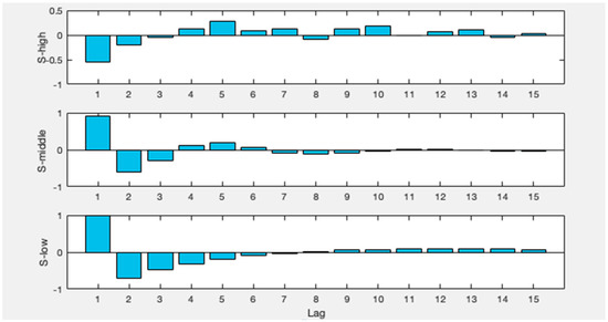
Figure 12.
The PACF results of Signal reconstruction by EEMD of “Yangdong Line.”
If the PACF at lag k was out of the 95% confidence interval, xi–k was applied as one of the input variables. Table 1 shows the PACF results for the four decomposition methods. In summary, Table 3 shows the input variables for predicting icing thickness.
Table 3.
Input factors selected by the PACF method of “Yangdong Line.”
3.4. Evaluation Indicators
In order to test the accuracy of the proposed CGWO-ELM model, the method of ELM, BP, GWO-ELM, GWO-BP were used as comparison models, and Root Mean Squared Error (RMSE) and R2 indices were used to verify them. The closer the value of R2 to 1, the smaller the value of RMSE, the higher the accuracy of the prediction will be;
: the i-th observed response value; : i-th fit response value; : response average.
Figure 13 explains the method used in the prediction of icing thickness in this paper, which is used to compare the superiority of various prediction models more clearly.
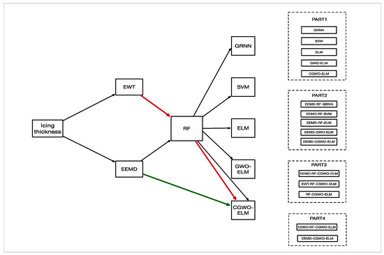
Figure 13.
Framework of the forecasting model comparisons.
In the part 1, five single prediction methods were gathered to show the necessity of introducing GWO and CGWO optimization algorithms; in part 2, EEMD-RF-GRNN, EEMD-RF-SVM, EEMD-RF-ELM, EEMD-RF-GWO-ELM, EEMD-CGWO-ELM were assembled for demonstrating the effectiveness of EEMD decomposition of ice thickness, and further illustrate the superiority of RF-CGWO-ELM optimization; in part 3, EEMD-RF-CGWO-ELM and EWT-RF-CGWO-ELM were used to reveal the progress in the application of the EEMD decomposition method in the decomposition of ice thickness; in part 4, the accuracy and effectiveness of the proposed RF factor selection algorithm was demonstrated by comparing EEMD-CGWO-ELM and EEMD-RF-CGWO-ELM.
4. Forecasting Results and Discussions of “Yangdong Line”
Figure 14 shows the prediction of icing thickness by 12 prediction models, and Table 4 shows the error analysis of 12 combined models. From this we can draw the following conclusions:
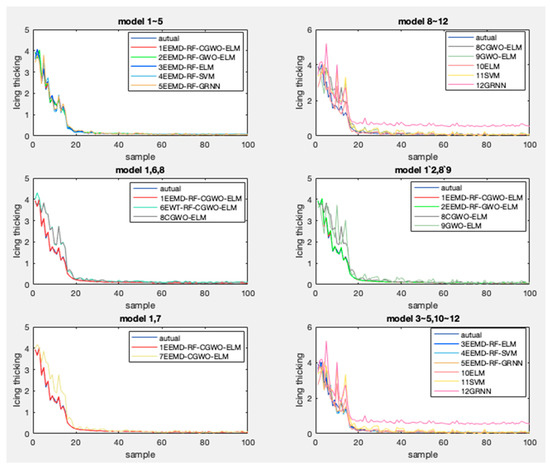
Figure 14.
Comparison of 12 prediction results of “Yangdong Line.”
Table 4.
Prediction method error analysis table of “Yangdong Line.”
- (a)
- Compared with other models, the EEMD-RF-CGWO-ELM model with lowest RMSE (0.864) and highest R2 (0.988) has higher accuracy for icing thickness prediction problems. It is very satisfactory that the model can be used to predict the thickness of icing.
- (b)
- In general, comparing the single model with the decomposed prediction model, the prediction accuracy of the single model is poor, which indicates that when the icing thickness is predicted, it is necessary to decompose the raw data of the icing thickness. The reason for this phenomenon is due to the strong instability/fluctuation/uncertainty of the icing thickness.
- (c)
- The accuracy of the EEMD-RF-CGWO-ELM model is more accurate than EWT-RF-CGWO-ELM, in other words, which has higher R2 and lower RMSE. It can be fully demonstrated that the effect of modal decomposition of icing thickness is better than the single data noise reduction because the noise of the original series of icing thickness is more serious, and the simple noise reduction process will have some errors in the prediction process.
- (d)
- Comparing models 1, 2 and models 8, 9, it can be found compared to the GWO model, that the R2 of the optimized GWO model is closer to 1, which is 0.988 and 0.917 while the GWO model is 0.972 and 0.913, respectively, and the RMSE is smaller with 0.864 and 2.86 respectively while the GWO model is 1.015 and 2.91. This is an indication that it is advisable to use the chaotic version of the GWO optimization model instead of the classic one.
- (e)
- Comparing EEMD-RF-CGWO-ELM and EEMD-CGWO-ELM, it is clear that, the prediction effect of the model was improved after the selection of eigenvectors using RF, indicating that RF feature selection can improve the effectiveness of the model.
- (f)
- Compared models 3–5 and models 10–12, compared to the GRNN and SVM models, ELM predictive model has a R2 closer to 1 and a smaller RMSE value, indicating that ELM is more suitable for carbon price prediction.
5. Additional Forecasting Case
In order to verify the universal applicability of the proposed model, which can help managers to predict the trend of icing thickness more accurately and make timely protective measures, this paper analyzes another situation of another transmission line.
The data of the 222 sets of high-voltage lines “front flat line 95” from 10 January 2008 to 15 February 2008 were selected for simulation prediction. The specific prediction method is consistent with the above, and now only a simple statement is made.
Figure 15 shows the trend of the icing thickness over time, including two short icing cycles, 1–104 for the first icing cycle and 105–222 for the second icing cycle.
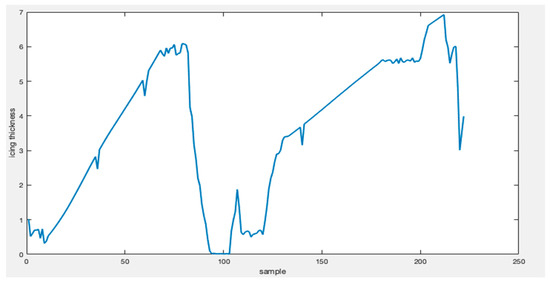
Figure 15.
The trend of icing thickness of “front flat line 95.”
To reduce the narrative, in the verification model, the decomposition of the data and the input selection are combined.
Figure 16 and Figure 17 show the results of EWT and EEMD decomposition of the raw data of the icing thickness, similarly, the icing thickness sequence is decomposed by EWT into myopic sequence A1 that can be selected for RF influencing factor analysis, PACF analysis, and prediction, and high frequency sequence D1 should be ignored. The eight sub-signals decomposed by EEMD were combined according to the frequency to obtain S-high (IMF 1 and IMF 2), S-middle (IMF 3 and IMF 4), and S-low (IMF 5~7 and R).
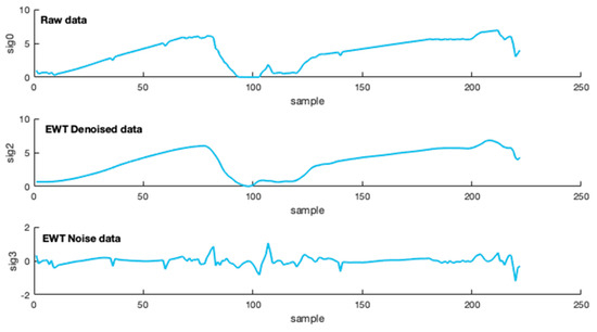
Figure 16.
EWT decomposition of “front flat line 95.”
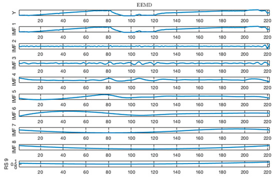
Figure 17.
EEMD decomposition of “front flat line 95.”
From the RF influencing factors of the decomposed sub-signals, it can be observed that the influencing factors 1, 3, 8, 5, 9 were selected as one of the inputs to the predicted A1 signal after the EWT decomposition. The influencing factors 1, 2, 3, 6, 8; 1, 2, 5, 6, 7; 1, 3, 4, 8, 9 were chosen as one of the inputs variables for the S-high signal, S-middle signal, S-low signal ice thickness forecasting after the decomposition of EEMD.
Figure 18 and Figure 19 show PACF results for sub-signals by two decomposition methods. Through the same calculation, the Lags could be determined as one of the inputs under the confidence level of 95%. Likewise, the corresponding Lags of three different frequency signals can be seen in Table 5.
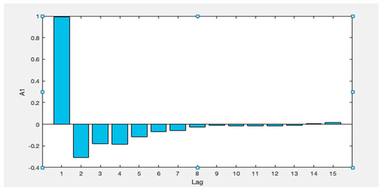
Figure 18.
The PACF results of A1 by EWT of “front flat line 95.”
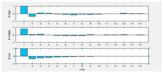
Figure 19.
The PACF results of signal reconstruction by EEMD of “front flat line 95.”
Table 5.
The input of ice thickness prediction of “front flat line 95.”
Figure 20 shows the prediction results of the 12 models for the icing thickness of “front flat line 95.” Table 6 shows the error analysis of 12 prediction models. Similarly, not only can we get similar to the above, we obtained three more conclusions.
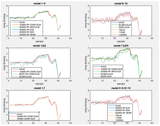
Figure 20.
Comparison of 12 prediction results of “front flat line 95.”
Table 6.
Prediction method error analysis table of “front flat line 95.”
- (a)
- The proposed method of EEMD-RF-CGWO-ELM still has the highest fit and the lowest RMSE among the 12 prediction methods so it can be well applied to the prediction of icing thickness. Although simulation of GRNN is still the worst, it produces relatively good results, which may be due to data differences.
- (b)
- For the decomposition of icing thickness by EEMD, undoubtedly, good results will be obtained. For example, comparing EEMD-RF-CGWO-ELM with RF-CGWO-ELM, the error index R2 and RMSE respectively increased by 0.06 and reduced by 1.6.
- (c)
- As far as the choice of RF influencing factors is concerned, the graphs and tables vividly reflect that we find the conclusion that using RF to select the influencing factors can promote the accuracy of the decomposition. For example, EEMD-RF-CGWO-ELM has better prediction accuracy than EEMD-CGWO-ELM.
6. Conclusions
A CGWO-ELM hybrid model based on EEMD decomposition, RF selection factors was proposed in this paper in order to make the icing thickness prediction more accurate. The icing thickness and related factors of Hunan transmission lines were selected for empirical analysis. Through the overall study, the following conclusions were obtained:
- (1)
- Compared with other methods, EEMD-RF-CGWO-ELM is a non-stationary and nonlinear innovative method for predicting the thickness of icing.
- (2)
- EEMD and RF factor analysis modeling can greatly improve the accuracy of prediction.
- (3)
- The forecast results show that the selected influencing factors are reasonable.
- (4)
- Two cases show that the model mentioned in this paper can help the power sector to deal with line ice accidents.
The intelligent learning algorithm proposed based on the influencing factors is of great significance for predicting the thickness of icing. It is satisfactory in urging relevant departments to take precautionary measures in advance and reduce the losses caused by disasters. Compared with previous research, this paper used EEMD to decompose icing thickness and used the RF method to select the influencing factors, which is a new breakthrough point.
Although the method proposed in this paper can predict the thickness of ice coating on short-term transmission lines, there are still some problems of concern. For example, during the melting of ice, the safe operation of the power grid will also be affected, so future research needs to consider the entire icing phase. On the other hand, the chaotic optimization of the grey wolf algorithm (CGWO) is not good for the optimization of complex functions. Therefore, the next research breakthrough can be used to introduce PSO into CGWO, which is applied to the optimization of complex functions, engineering optimization, and multi-objective problem solving.
Author Contributions
Investigation, W.W.; Methodology, D.Z.; Resources, D.Z.; Supervision, Y.J. and L.F.
Funding
This research was funded by the State Grid Corporation of China Science and Technology Project Funding, grant number [Nos. Kjgw2018-014].
Conflicts of Interest
The authors declare no conflict of interest.
References
- Li, X.J.; Xiong, H.X.; Yan, F.Z. Demand and Economic Analysis of Icing Observation for Power Planning and Design. Electr. Power Technol. Econ. 2011, 23, 14–18. [Google Scholar] [CrossRef]
- Hu, Y. Analysis and Countermeasures Discussion for Large Area Icing Accident on Power Grid. High Volt. Eng. 2008, 34, 215–219. [Google Scholar]
- Huang, X.B.; Liu, J.B.; Cai, W. Present Research Situation of Icing and Snowing of Overhead Transmission Lines in China and Foreign Countries. Power Syst. Technol. 2008, 32, 23–28. [Google Scholar]
- Yuan, J.H.; Liang, X.L.; Yi, H. The Present Study on Conductor Icing of Transmission Lines. High Volt. Eng. 2004, 30, 6–9. [Google Scholar] [CrossRef]
- Lan, D.L.; Zheng, Z.H. The Study on the Prediction Method of Ice Thickness of Transmission Line Based on The Combination of GRNN Neural Network. Electr. Eng. 2010, 27–30. [Google Scholar] [CrossRef]
- Ma, X.M.; Gao, J.; Wu, C. Prediction Model for Icing Thickness of Power Transmission Line Based on Grey Support Vector Machine. Electr. Power 2016, 49, 46–50. [Google Scholar] [CrossRef]
- Zhang, N.; Liu, T.J. Kernel function ELM method for short-term load forecasting considering influencing factors. Eng. J. Wuhan Univ. 2018, 51, 703–707. [Google Scholar] [CrossRef]
- Huang, Y.Y.; Mao, Y.; Lou, N.N. Short-Term Load Forecasting Based on Kohonen Clustering, Wavelet Packet Analysis and ELM Method. J. Nat. Sci. Hunan Norm. Univ. 2016, 39, 53–58. [Google Scholar] [CrossRef]
- Li, W.H.; Chen, Y.Z.; Guo, K. Parallel Extreme Learning Machine Based on Improved Particle Swarm Optimization. Pattern Recognit. Artif. Intell. 2016, 29, 840–849. [Google Scholar] [CrossRef]
- Zhong, W.; Li, C.X. Predicting of nonstationary downburst wind velocity based on extreme learning machines. J. Shanghai Univ. 2018, 24, 446–455. [Google Scholar] [CrossRef]
- Chen, L.J.; Li, H.H.; Li, F.Q. Short-term wind speed forecasting of combined ELM based on optimal clustering. Renew. Energy Resour. 2017, 35, 1841–1846. [Google Scholar] [CrossRef]
- Ding, J.L.; Liu, T.; Wang, J.L. KNN classification algorithm based on PSO-ELM feature mapping. Mod. Electron. Tech. 2019, 42, 152–156. [Google Scholar] [CrossRef]
- Lai, M.; Chen, G.B.; Liu, C. Boiler NOx Emission Prediction Based on a Hybrid Model of CAWOA and ELM. J. Chin. Soc. Power Eng. 2018, 38, 874–879. [Google Scholar]
- Tan, N.; Wang, X.S.; Huang, A.M. Wood Density Prediction of Cunninghamia lanceolata Based on Gray Wolf Algorithm SVM and NIR. Sci. Silvae Sin. 2018, 54, 137–141. [Google Scholar] [CrossRef]
- Yang, S.J.; Ye, X.; Li, J.S. BP Neural Network for Image Restoration Based on Grey Wolf Optimization Algorithm. Microelectron. Comput. 2018, 35, 19–22. [Google Scholar]
- Amjady, N.; Keynia, F.; Zareipour, H. A new hybrid iterative method for short-term wind speed forecasting. Eur. Trans. Electr. Power 2011, 21, 581–595. [Google Scholar] [CrossRef]
- Zhang, K.; Qu, Z.; Wang, J. A novel hybrid approach based on cuckoo search optimization algorithm for short-term wind speed forecasting. Environ. Prog. Sustain. Energy 2017, 36, 943–952. [Google Scholar] [CrossRef]
- Zhang, W.; Qu, Z.; Zhang, K. A combined model based on CEEMDAN and modified flower pollination algorithm for wind speed forecasting. Energy Convers. Manag. 2017, 136, 439–451. [Google Scholar] [CrossRef]
- Zhao, J.; Wang, J.; Liu, F. Multistep Forecasting for Short-Term Wind Speed Using an Optimized Extreme Learning Machine Network with Decomposition-Based Signal Filtering. J. Energy Eng. 2016, 142. [Google Scholar] [CrossRef]
- Wang, S.; Zhang, N.; Wu, L. Wind speed forecasting based on the hybrid ensemble empirical mode decomposition and GA-BP neural network method. Renew. Energy 2016, 94, 629–636. [Google Scholar] [CrossRef]
- Sun, W.; Liu, M. Wind speed forecasting using FEEMD echo state networks with RELM in Hebei, China. Energy Convers. Manag. 2016, 114, 197–208. [Google Scholar] [CrossRef]
- Liu, H.; Tian, H.; Liang, X. New wind speed forecasting approaches using fast ensemble empirical model decomposition, genetic algorithm, Mind Evolutionary Algorithm and Artificial Neural Networks. Renew. Energy 2015, 83, 1066–1075. [Google Scholar] [CrossRef]
- Mo, S.T.; Liu, T.Q.; Ceng, Q. Research on Accurate Prediction Model for Icing Thickness of Transmission Lines in Ultra-Short Period. Sichuan Electr. Power Technol. 2018, 41, 32–36. [Google Scholar]
- Huang, J.H.; Yan, J.; Wu, Q.H. Selective of informative metabolites using random forests based on model population analysis. Talanta 2013, 117, 549–555. [Google Scholar] [CrossRef] [PubMed]
- Hapfelmeier, A.; Ulm, K. A New Variable Selection Approach Using Random Forests. Comput. Stat. Data Anal. 2013, 60, 50–69. [Google Scholar] [CrossRef]
- Paul, J.; Dupont, P. Inferring statistically significant features from random forests. Neurocomputing 2015, 150, 471–480. [Google Scholar] [CrossRef]
- Wang, Y.Z. Prediction of Dam Deformation Based on EMD Neural Network Model. Water Power 2018, 44, 101–104. [Google Scholar]
- Zhao, Y.Z.; Nu, E.W.L.; Wu, S.E.S.L.M. Prediction Method of Network Traffic Based on Timing EEMD. Comput. Simul. 2018, 35, 466–469. [Google Scholar]
- Zhang, N.; Wang, P.; Bai, Y.P. Air Quality Prediction Based on MGWO-SVR. Math. Pract. Theory 2018, 48, 159–165. [Google Scholar]
- Yan, F.; Xu, J.Z.; Li, F.S. Training Multi-layer Perceptrons Using Chaos Grey Wolf Optimizer. J. Electron. Inf. Technol. 2019, 41, 872–879. [Google Scholar] [CrossRef]
- Zhang, H.Q.; Zhang, X.Y. Steam load forecasting based on chaos theory and LSSVM. Syst. Eng. Theory Pract. 2013, 33, 1058–1066. [Google Scholar] [CrossRef]
- Huang, G.B.; Zhu, Q.Y.; Siew, C.K. Extreme learning machine: A new learning scheme of feedforward neural networks. In Proceedings of the 2004 IEEE International Joint Conference on Neural Networks (IJCNN), Budapest, Hungary, 25–29 July 2004. [Google Scholar]
- Luo, J.X.; Luo, D.; Hu, Y.M. A new online extreme learning machine with varying weights and decision level fusion for fault detection. Control. Decis. 2018, 33, 1033–1040. [Google Scholar]
- Cao, X.H.; Liu, L.; Yang, P. The Research of Locomotion-Mode Recognition Based on Multi-Source Information and Extreme Learning Machine. Chin. J. Sens. Actuators 2017, 30, 1171–1177. [Google Scholar]
- Cui, D.L.; Guo, R. Random Forest Prediction Model and Its Application to Hydrology Based on Random Drift Particle Swarm Optimization. J. China Three Gorges Univ. 2019, 41, 6–10. [Google Scholar] [CrossRef]
- Ji, Y.J.; Guo, X.Y.; Liu, Y.L. Random Forest Based Quality Analysis and Prediction Method for Hot-Rolled Strip. Ournal Northeast. Univ. 2019, 40, 11–15. [Google Scholar] [CrossRef]
- Zhu, B.; Pan, L.L.; Zhou, Y. Fault probability calculation of transmission line considering ice melting factors. Power Syst. Prot. Control. 2015, 43, 79–84. [Google Scholar]


© 2019 by the authors. Licensee MDPI, Basel, Switzerland. This article is an open access article distributed under the terms and conditions of the Creative Commons Attribution (CC BY) license (http://creativecommons.org/licenses/by/4.0/).