Abstract
This paper presents a detailed description of data predictive control (DPC) applied to a demand-side energy management system. Different from traditional model-based predictive control (MPC) algorithms, this approach introduces two model-free algorithms of artificial neural network (ANN) and random forest (RF) to make control strategy predictions on system operation, while avoiding the huge cost and effort associated with learning a grey/white box model of the physical system. The operating characteristics of electrical appliances, system energy consumption, and users’ comfort zones are also considered in the selected energy management system based on a real-time electricity pricing system. Case studies consisting of two scenarios (0% and 15% electricity price fluctuation) are delivered to demonstrate the effectiveness of the proposed approach. Simulation results demonstrate that the DPC controller based on ANN pays only 0.18% additional bill cost to maintain users’ comfort zones and system economy standardization while using only 0.096% optimization time cost compared with the MPC controller.
1. Introduction
According to a report from the United States Energy Information Administration (EIA), about 39% of total US electricity was consumed by residential buildings in 2018 [1]. With the rapid development of intelligent building control algorithms, including predictive control and adaptive control strategy, it is practical and meaningful to put forward improvements in energy efficiency and energy management. Traditional predictive control algorithms, such as model predictive control (MPC) optimize future control actions at each time interval based on a selected physical system model. A model-based predictive control approach applied in building cooling systems with thermal energy storage was proposed in [2]. The proposed approach achieved lower electricity cost and better performance by optimizing the operation schedules of the central plant based on predictions of weather conditions and building loads. An application of fuzzy model predictive control (FMPC) in building heating control was presented in [3]. Disturbances of radiance, ambient temperature, and occupancy were considered in the FMPC-based building climate control system with regard to user comfort and monetary costs of heat supply. However, a widely recognized shortcoming of MPC is that it takes complicated and time-consuming procedures to capture a precise and accurate dynamic model of a physical system. There is always a gap between the optimization model and the realistic physical system. Moreover, traditional MPC is not suitable for applications with high frequency dynamics where the sampling time is measured in milliseconds or microseconds. Online optimization methods were implemented to improve the speed of MPC in [4]. The improved MPC computed the control actions for a problem with a horizon of 30 time steps in around 5 ms, which allowed MPC to be carried out at 200 Hz, while the algorithm stability required further analysis. Most of the existing model-based predictive methods perform better when the accuracy of modeling is higher. The MPC and rule-based control (RBC) method proposed in [5] outperformed robust model predictive control (RMPC) with regard to energy-comfort trade-off when the model uncertainty is less than 30% or more than 67%. The accuracy of the building models was found to be critical in the implementation of MPC algorithms [6]. However, higher costs and more efforts of constructing an accurate dynamics system result from the growing scale of industrial production and the additional sophistication of system structure in recent years. The expectation of an ideal control effect cannot be obtained with the classical model predictive control algorithm which creates an opportunity for model-free control methods [4]. Different from capturing a physics-based model, model-free control strategy is data-driven which relies on the input/output data of the selected system and does not need an explicit mathematical model. Previous studies [7,8,9] indicated that the neural network-based control strategies were effective in controlling a broad class of nonlinear processes. A data-driven adaptive control method based on the lazy learning (LL) technique for a class of discrete-time nonlinear systems were proved practical in [10]. The proposed LL-based controller is designed only using the input/output measurement data of the system by means of a pseudo gradient-based dynamic linearization technique. The robustness of the LL-based controller is verified to be enhanced due to the accurate prediction of the desired signal. The position tracking accuracy and processing efficiency of a non-circular cutting-derived Computer Numerical Control (CNC) system could be improved with a compact form dynamic linearization-based model-free adaptive predictive control method [11]. A neural network-based predictive control method was introduced to solve the tracking problems of a nonlinear system successfully in [12]. Moreover, multiple authors applied recurrent neural network algorithms in the domain of building energy predictions successfully [13,14,15,16]. Similar research was carried out on applying model-free methods to assisting system control operations [17,18,19]. Ref. [20] highlighted that model-free data-based control methods were practical in industrial practice if online calibration were to be performed. The concept of data predictive control (DPC), an alternative approach using control-oriented data-driven models for implementing receding horizon control, was mentioned in [21]. The proposed control-oriented data-driven model uses two algorithms of a single regression tree and random forest to control system inputs and disturbances. The inputs and disturbances of a selected building model are separated into controllable variables and uncontrollable ones. This separation method is called recursive partitioning, which improves the performance of the system response prediction. Jain et al. [21] demonstrated that DPC was a practical alternative to MPC in trading off energy consumption against thermal comfort without taking a real-time electricity pricing system into consideration. The primary reason for the modeling choice in [21] was that complicated models like neural network went through a longer calculation routine and involved more factors, which put up barriers for an engineer to judge whether the operation was correct or not, than interpretable regression trees. However, Ahmad et al. [22] compared the performance of artificial neural network (ANN) with random forest (RF) for the hourly HVAC energy consumption prediction of a hotel. The results proved that both models had comparable predictive power and nearly equal applicability in building energy applications. Ahmad et al. pointed out that ANN models were good choices to be used as surrogate models instead of detailed dynamic simulation models in real-time control applications. Moreover, ANN performed marginally better than RF with a lower root-mean-square error (RMSE) in general [22].
In this paper, a novel DPC method is applied to an energy management system. Two model-free algorithms of ANN and RF are selected to make control strategy predictions for a system operation, while avoiding the huge cost and effort associated with learning a grey/white box model of the physical system. Due to the difficulty in obtaining original system operation data and the lack of sensors to provide real-time measurements, a model-based predictive control method is selected as a classical and practical benchmark to produce previous information of electrical appliances in the energy management system [23].
The contributions of this paper are summarized as below:
- This paper presents a full picture of the DPC method based on ANN and RF algorithms. An MPC method using a precise dynamic model based on a design code for civil buildings of China is utilized to produce the original system operation data, which serve as the training data for the machine learning algorithms, while avoiding the costs and efforts of system measurements.
- The proposed method takes the operating characteristics of electrical appliances, system energy consumption, users’ comfort zones, and electricity price fluctuation into consideration based on a real-time electricity pricing system. The remarkable performance of the proposed ANN-based DPC algorithm in saving simulation time cost and in trading off energy cost with comfort is validated in the energy management system considering electricity price fluctuation.
The rest of the paper is organized as follows. Section 2 presents the infrastructure of the proposed energy management system. Section 3 presents the construction of the model predictive control. Section 4 introduces the scheme of the proposed data predictive control method. Section 5 demonstrates the effectiveness of the proposed DPC with two case studies and the conclusion is drawn in Section 6.
2. System Overview
Considering a typical building model of an energy management system with electric heaters (EHs) and basic user loads, a schematic diagram of the proposed energy management system is shown in Figure 1. The model is a four-story northeast-facing building consisting of 16 household electric heaters and basic user loads, which consist of lighting equipment, computers, printers, televisions, and refrigerators. Each layer is considered as a 400 square meter and 3 m high single apartment with four uniform electric heaters and basic loads. The electric heaters are used to adjust indoor temperature to maintain the users’ comfort zone. The basic loads of each layer have a similar pre-set 24 h fixed power curve. The average power cost of the basic loads on each layer is 110.31 kWh per day. The rating power of each electric heater is 2 kW. The total area of windows on each layer is 10 square meters. Heat exchange between indoor and outdoor environments through the walls, windows, ground, and roof which influences the indoor temperature is also considered. The meagre internal heat gains produced by basic loads and human activities are ignored. The orientation correction factor of the northeast-facing building model located at Beijing is set as 0% according to the Design Code for Heating, Ventilation, and Air Conditioning of Civil Buildings [24]. The environmental seasonal condition is set as winter. The hourly outdoor temperature data is collected from China Weather Reuters.
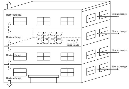
Figure 1.
Schematic diagram of energy management system.
Based on the proposed building model with temperature data and pre-acquired electricity price data, an MPC scheme is designed to minimize the electricity cost to keep users’ comfort. The output predictive control strategies of the MPC module represent the schedule of EHs over a specified time period. With the historical control strategies provided by the MPC module, a DPC scheme is proposed to compensate the modeling errors, especially parameter error and measurement error, when designing the structure-based physical system model. Model-free algorithms of ANN and RF are applied to make control strategy prediction in the DPC module. The electricity cost and time cost of the proposed MPC and DPC algorithms are evaluated under the limitation of users’ comfort zones. A summarization of the operational data used in MPC and DPC modules is presented in Figure 2.
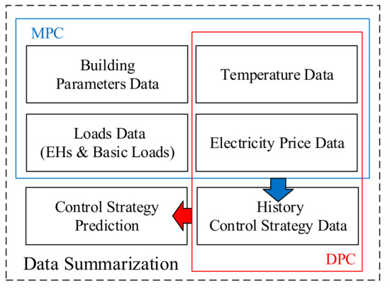
Figure 2.
Summarization of the operational data used in Model Predictive Control (MPC) and Data Predictive Control (DPC).
3. Model Predictive Control
Based on the proposed system model and the modeling approach of household heating and cooling appliances in Zhou, Zhang, and Yang’s study [25], the temperature increment in a unit time segment is shown in the following function:
where is the temperature variable quantity, is the unit time, is number of electric heaters working at time t, is the rating power of electric heaters, is the area of each layer, is the height of each layer, is the air density, and is the specific heat capacity.
Equation (2) describes the difference between the indoor and outdoor temperatures which relate to the temperature of the previous time segment:
where is the indoor temperature, is the outdoor temperature, and is the temperature difference between them.
Based on Equations (1) and (2), the indoor temperature can be deduced in the following function:
In this paper, construction of each layer is considered as a building envelope. The heat consumption of a building envelope is defined in Equation (4).
where is the heat consumption of the building envelope, is the thermal transfer coefficient, and is the thermal exchange area (e.g., ,,,).
The proposed model is aimed at minimizing the energy usage by dispatching the electric heaters while maintaining a desired level of thermal comfort and considering the varying electricity price. The idea indoor temperature is set as , with deviation in winter, according to the evaluation criterion of thermal comfort in [24]. The optimization function is defined as follows:
where is the real-time electricity price, is the basic user loads at time t, is the rating power of electric heaters, is the thermal comfort parameter, is a pre-set comfortable interior temperature parameter, is the unit time, and is number of active electric heaters per floor at time t.
It is assumed in this paper that is the key variable which has a great influence on both temperature difference and users’ comfort zones for electric heating systems. The core of the proposed model predictive control is building a practical model by introducing strategy-concerned control variables to realize the balance of energy usage and users’ comfort zones for energy management systems. Thus, is noted as an important control variable in the electric heating system at time t. In this paper, the value of will be passed to the DPC model as past control strategy data for further control strategy forecasting.
For the proposed nonlinear system, the widely used performance indices are based on the infinite horizon which maintains the closed loop stability over all time intervals [26]. Thus, the finite receding horizon control (RHC) method is applied to the proposed model optimization. The schematic diagram of the RHC method is presented in Figure 3. At time t, the optimization problem is solved over a future horizon of N steps. Only the first optimal move is applied, while the rest of the sequence is thrown away. At time t + 1, the window will move one step forward, while the optimization repeats with new measurements of and .
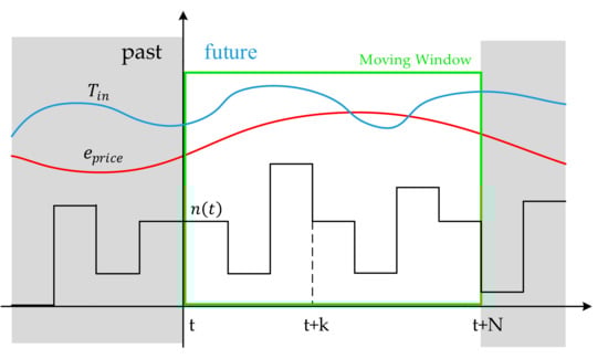
Figure 3.
Schematic diagram of the infinite receding horizon control (RHC).
4. DPC
The purpose of data predictive control is to provide a practical model by using past measurement data (e.g., past control strategy data and past temperature data) to control the inputs and disturbances, instead of building a physics-based model with imprecise parameters. The past temperature data was collected from China Weather Reuters. The past control strategy data was provided by the optimization results of MPC. Figure 4 presents the schematic diagram of DPC.
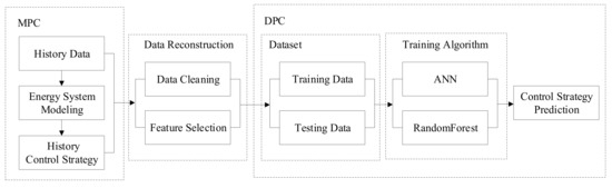
Figure 4.
Schematic diagram of DPC.
Due to the difficulties in acquiring the actual work-date data of a certain energy system, a typical model of a four-story building is deployed, consisting of 16 electric heaters and basic user loads, as described in Section 2. The past outdoor temperature data, real-time electricity price, and basic loads are recognized as the input past data of the MPC module. The value of the control variable at all working conditions is treated as the past control strategy data once the MPC module is optimized, according to the constraints proposed by Jin and Liu [7]. After reasonable data cleaning and selection of essential features over the output of MPC module, the reconstructed data is split into training data and testing data. Based on machine learning algorithms, including ANN and RF, prediction of future control strategy is performed.
The DPC strategy brings several advantages: (1) Complex and time-consuming measurements of structure dependent system parameters are avoided by using the predictions made by the estimators; (2) good initial estimate of parameters is not necessary for the optimization procedure; (3) time cost of the optimization procedure for finding suitable control strategies is saved.
4.1. DPC Based on ANN
To build a data predictive controller, real-time electricity price, controller data, and outdoor temperature data of Beijing from January to February in 2017 were selected as features for training the ANN model. The total feature variables are listed as follows:
- (1)
- Natural Resource Data: This includes measurements of outdoor air temperature .
- (2)
- Controller Data: This includes history values of control variable collected from MPC optimization results.
- (3)
- Electricity Price Data: This includes values of history real-time electricity price .
We learn an ANN model which predicts future controller data with the given past natural resource data, controller data, and electricity price data:
where is past measurements of outdoor air temperature, is previous control strategy data collected from the optimization results of the MPC procedure, is past real-time electricity price, is the output of the ANN model, and N is a preset input constant.
The network model uses the square error loss function to evaluate the distance difference between the target value and the predicted value, which allows candidate solutions of the training procedure to be ranked and compared:
where is the true value of the real target, is the predicted value of the target, is the weights of the input layer and the hidden layer, is an L2-regularization term that penalizes complex models, and is a non-negative hyper parameter that controls the magnitude of the penalty.
The proposed model is a three-layer feed backward neural network with one hidden layer which contains 50 neurons. The input and output layers have 72 and 24 neurons, respectively. The activation function of rectified linear units is applied in the network. The constant parameter of tolerance for convergence is set to 0.0001. The Adam optimization algorithm, which performs well in bias-correction across different hyperparameter settings, is selected as the stochastic optimizer [27].
Thus, a predictive control scheme is designed based on the data dependent modeling method. The whole structure of the control strategy based on ANN can be seen in Figure 5.
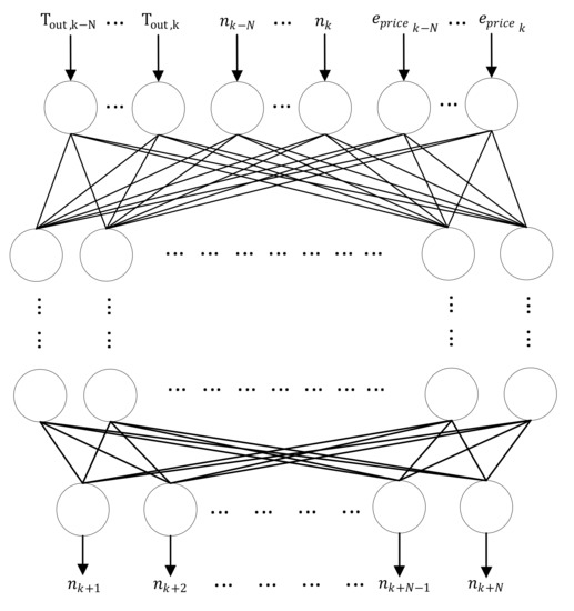
Figure 5.
Structure of the ANN.
4.2. DPC Based on RF
The RF introduced by Leo Breiman [28] is one of the ensemble learning algorithms developed for building classification or regression models. The core of the RF algorithm is to build classification or regression trees using bootstrapped samples of original data which are usually split into training and testing data at a ratio of 2:1. Each decision tree of the forest makes a classification or prediction of selected target features at leaves until the end of each loop. Once all the trees are built and the training procedure is accomplished, a majority vote is held to determine the final result of the original classification or prediction problem by all the individual trees in the forest. The out-of-bag error or mean square error (MSE) is measured to evaluate the performance of the entire forest. The structure of the RF algorithm is shown in Figure 6.
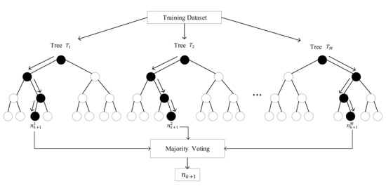
Figure 6.
Structure of the random forest algorithm.
The RF is composed of ensemble regression trees , where is an input feature vector bootstrapped from the training dataset. The outputs of ensemble trees are , where is the value of control strategy at time k + 1 predicted by the ith tree. The number of estimators (trees) in the proposed forest is set to 100. In the end, the individual regression tree makes a majority voting to produce an averaged outcome of the RF prediction.
In comparison with ANN, the proposed RF model is considered as a white box that the accuracy of classification or regression operation at the leaves is easy to understand and interpret. Multiple parameters and complex structures of a neural network result in long circle calculation and adjustment. In contrast, the number of estimators or decision trees is usually the essential element that an RF algorithm needs to focus on. Numerous input parameters of the proposed system can be handled with a built-in feature evaluation system of the RF algorithm, while the neural network has to delete some unnecessary parameters to reduce dimensionality by data cleaning and feature selection.
5. Case Studies
Simulations are performed to test the performance of the proposed DPC algorithm against the MPC algorithm. The quantitative analysis of the electricity cost for DPC controller and MPC controller is presented in this section. The performance of ANN-based DPC and random forest-based DPC is discussed. Since there is always a gap between the predicted electricity price data value and the actual data value, the fluctuation of the real-time electricity price has a consequential effect on bill computation. A random variable ranging from 0% to 15% is set to compensate for the influence of fluctuation. The training data of electricity price is revised to . The optimization function in Equation (5) is modified as the following:
Figure 7 shows the 24 h history electricity price data from January to February in 2017. The reasons for the negative value of electricity price on 9 January can be listed as follows: (1) The cost of shutting down or starting up generators overwhelms the loss of profits caused by providing electricity subsidies to terminal users and (2) the power plant is obliged to provide re-dispatch power or contracted balancing power to maintain the stability of the grid. For the modeling of the MPC controller and the DPC controller, Python is selected as the programming language and Gurobi is used as the optimization solver.
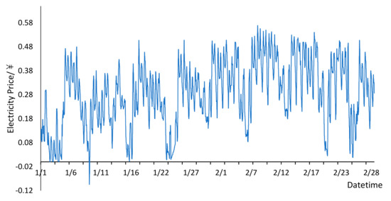
Figure 7.
Electricity price data from January to February in 2017.
5.1. Case I: DPC Based on ANN (15% Electricity Price Fluctuation)
To evaluate the performance of the proposed ANN-based DPC controller against the MPC controller, the history controller data obtained by MPC optimization, real-time electricity price, and hourly outdoor temperature of Beijing from January to February collected from China Weather Reuters are selected as input feature variables for training the ANN model. Aiming to perform a comprehensive analysis on the DPC controller, the electricity price fluctuation at 0% and 15% are analyzed respectively.
Figure 8 presents the comparison of the output controller data predicted by the ANN model and actual controller data collected from MPC controller without taking the fluctuation of electricity price into consideration. The y axis represents the total number of active electric heaters. The x axis represents the preset 24 time-intervals during a day. The red curve shows the number of active heaters predicted by the DPC controller based on ANN. The blue curve shows the number of heaters which are supposed to be turned on by MPC controller. In this paper, the prediction accuracy () is defined to evaluate the prediction result of the DPC controller (when the difference between the number of heaters predicted by DPC controller and the number provided by MPC controller is beyond 1, the DPC predicted data at that time is supposed to be incorrect or unreasonable. represents the number of time points with correctly predicted EHs and denotes the total number of time points of a day, which is 24). It can be seen that the accuracy of heaters number predicted by the DPC controller based on ANN reach approximately 70% when the result of MPC controller data is considered as standardization.
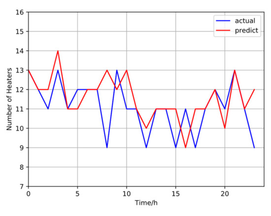
Figure 8.
Prediction of DPC controller based on ANN (0% electricity price fluctuation).
Figure 9 illustrates the prediction results of ANN and MPC when the fluctuation of electricity price is 15%. The prediction accuracy of ANN-DPC is about 75% percent when compared to the result of MPC.
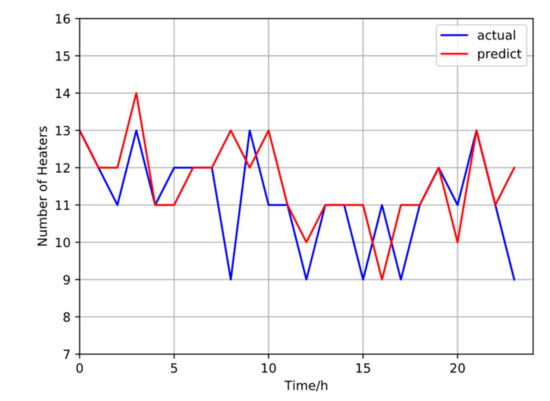
Figure 9.
Prediction of DPC controller based on ANN (15% electricity price fluctuation).
Table 1 provides a summary of numerical analysis on prediction result of DPC controller.

Table 1.
Numerical summary of ANN-based DPC controller.
From Table 1, it can be found that the accuracy of the DPC controller prediction is up to 70% without taking electricity price fluctuation into consideration. For the scenario of 15% electricity price fluctuation, the accuracy of DPC increases by 5% and the value of RMSE decreases approximately by 6% when compared with the prediction accuracy of 0% electricity price fluctuation.
To further evaluate the prediction result of DPC controller with regard to users’ comfort zones, the number of active electricity heaters predicted by ANN-DPC is substituted back to calculate the indoor temperature variation for each floor. Figure 10 shows the average indoor temperature variation curve of the proposed four-story system when the electricity heaters are scheduled according to the prediction result of DPC in Figure 8. For the scenario of 15% electricity price fluctuation, the indoor temperature variation on average is pictured in Figure 11.
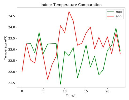
Figure 10.
Indoor temperature comparison (ANN-DPC, 0% electricity price fluctuation).
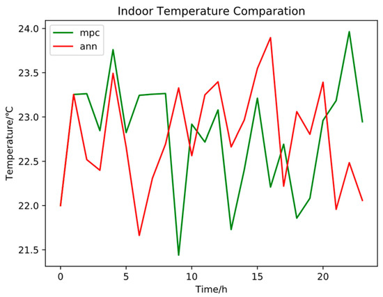
Figure 11.
Indoor temperature comparison (ANN-DPC, 15% electricity price fluctuation).
Table 2 provides a summary of numerical analysis on indoor temperature variation caused by electricity heaters which are scheduled under the arrangement of ANN-DPC controller. The green curve in Figure 10 and Figure 11 denotes the indoor temperature under MPC controller at each time interval. For the scenario of 15% electricity price fluctuation, the value of Mean Square Error (MSE) improves by 5.5% and Mean Absolute Percentage Error (MAPE) decreases by 32.5% when compared with the values of 0% electricity price fluctuation.
Table 2.
Numerical summary of indoor temperature variation (ANN-DPC).
To further indicate the advantages of applying data predictive control methods to building energy management systems, the electricity cost and the time cost to accomplish the optimization of control strategy is listed in Table 3.
Table 3.
Bill and time cost comparison between ANN-DPC and MPC.
The total electricity cost of using the MPC controller to schedule the electric heaters at 24 time-intervals is 176.9266, while the bill of the DPC controller without considering electricity price fluctuation is 3.92% more than MPC controller. The results reveal that the MPC controller with precise and detailed physical models performs better in saving bills than DPC controller. However, the time cost of the MPC controller to accomplish the whole optimization circle is over 300 s, which is about 1300 times the cost of the DPC controller.
For the scenario of 15% electricity price fluctuation, the ANN-DPC costs only 0.18% additional bill over MPC. At the same time, the time cost of ANN-DPC controller is about 0.2882 s, which is 0.096% of the time MPC costs.
According to the analysis above, it can be concluded that the performance of the proposed ANN-DPC controller is reasonable with regard to different electricity fluctuation. Applying an ANN-DPC controller rather than an MPC controller into the energy management system is a better choice to trade off energy and comfort when the real-time requirement is highlighted in the system.
5.2. Case II: DPC Based on RF (15% Electricity Price Fluctuation)
To evaluate the performance of the proposed random forest algorithm, a comprehensive numerical analysis for the DPC based on random forest is conducted in this section. It should be noted that the real-time electricity price and hourly outdoor temperature of Beijing from January to February in 2017 collected from China Weather Reuters and the past controller data collected from MPC optimization results are also used as input features for training the random forest model. The impact of electricity price fluctuation on prediction control based on random forest is also analyzed.
Figure 12 shows the comparison of the output control strategy data predicted by the random forest model and original control strategy data collected from the MPC controller with 0% electricity price fluctuation. For the scenario of 15% electricity price fluctuation, the prediction performance is presented in Figure 13.
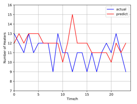
Figure 12.
Prediction of RF-DPC (0% electricity price fluctuation).
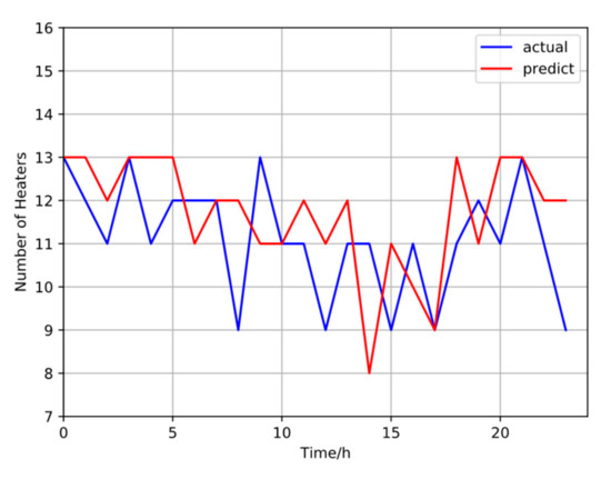
Figure 13.
Prediction of RF-DPC (15% electricity price fluctuation).
From Figure 12, it can be seen that the red curve which represents the prediction of the random forest-based DPC shows almost the opposite results against MPC. The performance of RF is far from satisfactory without taking electricity price fluctuation into consideration. However, the prediction result is improved with 15% electricity price fluctuation in Figure 13. To comprehensively demonstrate the difference between the prediction results of DPC and MPC, Table 4 shows a summary of the numerical analysis on the results predicted by RF-based DPC.
Table 4.
Numerical summary of RF-DPC.
From Table 4, the accuracy value of the RF-DPC prediction decreased by 13.5% when the influence of electricity price variation is considered in the system, while the value of RMSE is improved by 14.98%. Considering the fact that a single unit change in is associated with a deviation of 4.1% in , the accuracy of RF-DPC with 15% fluctuation is acceptable. Compared with the RMSE of ANN-DPC with 15% fluctuation, the value of RMSE in RF-DPC increases by 32.9%, which reveals the poor performance of RF in dealing with uncontrollable random noise like electricity price fluctuation. Figure 14 shows the average indoor temperature variation curve of the proposed building model when the electricity heaters are scheduled according to the prediction result of DPC controller in Figure 11. The scenario of 15% electricity price fluctuation is presented in Figure 15.
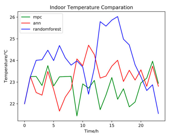
Figure 14.
Indoor temperature comparison (RF-DPC, 0% electricity price fluctuation).
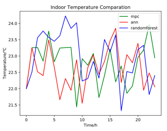
Figure 15.
Indoor temperature comparison (RF-DPC, 15% electricity price fluctuation).
From Figure 14, the indoor temperature calculated by RF-DPC is over at the 15th time interval. The indoor temperature difference between RF-DPC and MPC is which exceeds the users’ comfort zone limit of . For the scenario of 15% electricity price fluctuation, the improved performance of RF-DPC in an energy-comfort trade-off is demonstrated in Figure 15.
Table 5 provides the summary of numerical analysis on indoor temperature variation caused by electricity heaters, which are scheduled under the arrangement of RF-DPC controller. For the scenario of 15% electricity price fluctuation, the value of MSE is enhanced by 11.1% when compared with ANN-DPC.
Table 5.
Numerical summary of indoor temperature variation (RF-DPC).
The bill of electricity cost and the time cost of RF-DPC is listed in Table 6. The bill cost of RF-DPC with 15% electricity price fluctuation is 3.39% more than the MPC’s. The time cost of RF-DPC controller reaches about 0.3 s, which is 0.1% of that of MPC, equivalent to the time cost of ANN-DPC.
Table 6.
Bill and time cost comparison between RF-DPC and MPC.
According to the analysis above, it can be concluded that the performance of the proposed RF-DPC controller is acceptable only at the scenario of 15% electricity price fluctuation. By paying an additional bill cost of 3.39% and 0.1% time cost against MPC, the RF-DPC achieves the goal of trading off energy cost and users’ comfort. For the same scenario, the ANN-DPC has a better performance by paying only 0.18% additional bill cost and 0.096% time cost against MPC.
6. Conclusions
This paper assesses the structure of the data predictive control (DPC) algorithm with the example of building an energy management system by using the model predictive control (MPC) method. The operating characteristics of electrical appliances, system energy consumption, and users’ comfort zones are also considered in this system based on a real-time electricity pricing system. Two machine learning algorithms of artificial neural network (ANN) and random forest (RF) are deployed to perform controller strategy prediction and to verify the possibility of reducing the impact of electricity price fluctuation. Numerical analysis is conducted on two essential elements of electricity bill cost and optimization time cost. For the scenario of 15% electricity price fluctuation, the analysis reveals the poor performance of random forest in dealing with uncontrollable random noise like electricity price fluctuation. Moreover, RF-DPC pays 3.39% additional bill cost and 0.1% time cost against MPC, while the ANN-DPC pays only 0.18% additional bill cost and 0.096% time cost against MPC. It is found that the data predictive control strategy is a better choice when real-time requirement is highlighted in the system operation.
Author Contributions
Conceptualization, W.G. and S.Z.; methodology, F.Z.; validation, S.Z. and F.Z.; formal analysis, F.Z.; Writing—review & editing, Z.W.
Funding
This research was jointly supported by National Natural Science Foundation of China under Grant 51807024 and Jiangsu Key Laboratory of Smart Grid Technology and Equipment.
Conflicts of Interest
The authors declare no conflict of interest.
Nomenclature
| The temperature variable quantity. | |
| The unit time. | |
| Number of active electric heaters at time t. | |
| The rating power of electric heaters. | |
| The area of each layer. | |
| The height of each layer. | |
| The air density. | |
| The specific heat capacity. | |
| The indoor temperature. | |
| The outdoor temperature. | |
| The temperature difference between indoor and outdoor temperature. | |
| The heat consumption of building envelope. | |
| The thermal transfer coefficient. | |
| The thermal exchange area. | |
| Real-time electricity price at time t. | |
| Power of basic loads at time t. | |
| The thermal comfort parameter. | |
| A pre-set comfortable interior temperature parameter. | |
| The square error loss function. | |
| The weights of the input layer and the hidden layer. | |
| A non-negative hyper parameter. | |
| A fluctuation-relevant random variable. | |
| The prediction accuracy. | |
| The number of time points with correctly predicted electric heaters. | |
| The total number of time points of a day. |
References
- U.S. Energy Information Administration. Electric Power Monthly with Data for February 2019. Available online: https://www.eia.gov/electricity/monthly/current_month/epm.pdf (accessed on 1 April 2019).
- Ma, Y.; Borrelli, F.; Hencey, B.; Coffey, B.; Bengea, S.; Haves, P. Model Predictive Control for the Operation of Building Cooling Systems. IEEE Trans. Control Syst. Technol. 2011, 20, 796–803. [Google Scholar]
- Mayer, B.; Killian, M.; Kozek, M. Cooperative and Hierarchical Fuzzy MPC for Building Heating Control. In Proceedings of the 2014 IEEE International Conference on Fuzzy Systems (FUZZ-IEEE), Beijing, China, 6–11 July 2014; pp. 1054–1059. [Google Scholar]
- Wang, Y.; Boyd, S. Fast Model Predictive Control Using Online Optimization. IEEE Trans. Control Syst. Technol. 2009, 18, 267–278. [Google Scholar] [CrossRef]
- Maasoumy, M.; Razmara, M.; Shahbakhti, M.; Vincentelli, A.S. Handling Model Uncertainty in Model Predictive Control for Energy Efficient Buildings. Energy Build. 2014, 77, 377–392. [Google Scholar] [CrossRef]
- Serale, G.; Fiorentini, M.; Capozzoli, A.; Bernardini, D.; Bemporad, A. Model Predictive Control (MPC) for Enhancing Building and HVAC System Energy Efficiency: Problem Formulation, Applications and Opportunities. Energies 2018, 11, 631. [Google Scholar] [CrossRef]
- Jin, N.; Liu, D. Discrete-Time/SPL Epsilon/-Adaptive Dynamic Programming Algorithm Using Neural Networks. In Proceedings of the 2008 IEEE International Symposium on Intelligent Control, San Antonio, TX, USA, 3–5 September 2008; pp. 1085–1090. [Google Scholar]
- Noriega, J.R.; Wang, H. A Direct Adaptive Neural-Network Control for Unknown Nonlinear Systems and its Application. IEEE Trans. Neural Netw. 1998, 9, 27–34. [Google Scholar] [CrossRef] [PubMed]
- Liu, D.; Jin, N. Finite Horizon Discrete-Time Approximate Dynamic Programming. In Proceedings of the 2006 IEEE Conference on Computer Aided Control System Design, 2006 IEEE International Conference on Control Applications, 2006 IEEE International Symposium on Intelligent Control, Munich, Germany, 4–6 October 2006; pp. 446–451. [Google Scholar]
- Hou, Z.; Liu, S.; Tian, T. Lazy-Learning-Based Data-Driven Model-Free Adaptive Predictive Control for a Class of Discrete-Time Nonlinear Systems. IEEE Trans. Neural Netw. Learn. Syst. 2016, 28, 1914–1928. [Google Scholar] [CrossRef] [PubMed]
- Junwei, D.; Rongmin, C.; Zhongsheng, H.; Yunjie, Z. Model-free Adaptive Predictive Control for Non-Circular Cutting Derived CNC System. In Proceedings of the 2016 Chinese Control and Decision Conference (CCDC), Yinchuan, China, 28–30 May 2016; pp. 5772–5777. [Google Scholar]
- Dong, N.; Liu, D.; Chen, Z. Data Based Predictive Control Using Neural Networks and Stochastic Approximation. In Proceedings of the 2011 International Conference on Modelling, Identification and Control, Innsbruck, Austria, 14–16 February 2011; pp. 256–260. [Google Scholar]
- Kalogirou, S.A.; Bojic, M. Artificial Neural Networks for the Prediction of the Energy Consumption of a Passive Solar Building. Energy 2000, 25, 479–491. [Google Scholar] [CrossRef]
- Kreider, J.F.; Claridge, D.E.; Curtiss, P.; Dodier, R.; Haberl, J.S.; Krarti, M. Building Energy Use Prediction and System Identification using Recurrent Neural Networks. J. Sol. Energy Eng. 1995, 117, 161–166. [Google Scholar] [CrossRef]
- Yan, C.; Yao, J. Application of ANN for the Prediction of Building Energy Consumption at Different Climate Zones with HDD and CDD. In Proceedings of the 2010 2nd International Conference on Future Computer and Communication, Wuhan, China, 21–24 May 2010; Volume 3, pp. V3-286–V3-289. [Google Scholar]
- Azadeh, A.; Ghaderi, S.F.; Sohrabkhani, S. Annual Electricity Consumption Forecasting by Neural Network in High Energy Consuming Industrial Sectors. Energy Convers. Manag. 2008, 49, 2272–2278. [Google Scholar] [CrossRef]
- Li, H.; Yamamoto, S. A Model-free Predictive Control Method Based on Polynomial Regression. In Proceedings of the 2016 SICE International Symposium on Control Systems (ISCS), Nagoya, Japan, 7–10 March 2016; pp. 1–6. [Google Scholar]
- Dinh, T.Q.; Marco, J.; Greenwood, D.; Ahn, K.K.; Yoon, J.I. A Data-based Hybrid Driven Control for Networked-Based Remote Control Applications. In Proceedings of the 2017 IEEE International Conference on Mechatronics (ICM), Gippsland, Australia, 14–17 February 2017; pp. 382–387. [Google Scholar]
- Anderlini, E.; Forehand, D.I.; Stansell, P.; Xiao, Q.; Abusara, M. Control of a Point Absorber Using Reinforcement Learning. IEEE Trans. Sustain. Energy 2016, 7, 1681–1690. [Google Scholar] [CrossRef]
- Abouaissa, H.; Hasan, O.A.; Join, C.; Fliess, M.; Defer, D. Energy Saving for Building Heating Via a Simple and Efficient Model-Free Control Design: First Steps with Computer Simulations. In Proceedings of the 2017 21st International Conference on System Theory, Control and Computing (ICSTCC), Sinaia, Romania, 19–21 October 2017; pp. 747–752. [Google Scholar]
- Jain, A.; Behl, M.; Mangharam, R. Data Predictive Control for Building Energy Management. In Proceedings of the 2017 American Control Conference (ACC), Seattle, WA, USA, 24–26 May 2017; pp. 44–49. [Google Scholar]
- Ahmad, M.W.; Mourshed, M.; Rezgui, Y. Trees Vs Neurons: Comparison Between Random Forest and ANN for High-resolution Prediction of Building Energy Consumption. Energy Build. 2017, 147, 77–89. [Google Scholar] [CrossRef]
- Chen, C.; Wang, J.; Heo, Y.; Kishore, S. MPC-based Appliance Scheduling for Residential Building Energy Management Controller. IEEE Trans. Smart Grid 2013, 4, 1401–1410. [Google Scholar] [CrossRef]
- National Standard of the People’s Republic of China. GB 50736-2012: Design Code for Heating Ventilation and Air Conditioning of Civil Buildings; Architecture Building Press: Beijing, China, 2012. [Google Scholar]
- Zhou, S.; Zhang, X.P.; Yang, X. Design of Demand Management System for Household Heating Cooling. In Proceedings of the 2012 3rd IEEE PES Innovative Smart Grid Technologies Europe (ISGT Europe), Berlin, Germany, 14–17 October 2012; pp. 1–6. [Google Scholar]
- Mayne, D.Q.; Michalska, H. Receding Horizon Control of Nonlinear Systems. IEEE Trans. Automat. Control 1990, 35, 814–824. [Google Scholar] [CrossRef]
- Kingma, D.P.; Ba, J. Adam: A Method for Stochastic Optimization. arXiv 2014, arXiv:1412.6980. [Google Scholar]
- Breiman, L. Random Forests. Mach. Learn. 2001, 45, 5–32. [Google Scholar] [CrossRef]


© 2019 by the authors. Licensee MDPI, Basel, Switzerland. This article is an open access article distributed under the terms and conditions of the Creative Commons Attribution (CC BY) license (http://creativecommons.org/licenses/by/4.0/).