Abstract
While variable renewable energy (VRE) has been developed for decades, VRE market participation is developing relatively slowly, despite the potential economic efficiency it may bring. This paper tries to specify the efficiency of VRE in a deregulated pool-based electricity market. Based on standard pool-based market design, this paper built a direct current optimal power flow (DC-OPF) based simplified 2-settlement spot electricity market model conjugating electricity and ancillary service clearing. To address the outcomes of the imperfect market in the real world, this paper studied the consequences brought by agents’ learning and strategic behaviors. Simulations under different ancillary service levels and reliability cost levels are carried out. The results show that VRE may be unprofitable in the market, especially when learning and strategic behavior is considered. Learning and strategic market behavior will also hamper the role of VRE as a “better” energy source. This paper shows and proves a locational marginal price (LMP) disadvantage phenomenon, which will lead to low profitability of VRE. Three major suggestions are given based on the results.
1. Introduction
Variable renewable energies (VREs) such as photovoltaic (PV) and wind have become important sources of renewable and clean energy. The installed capacity quantities of PV and wind have reached 161.96 GW and 245.83 GW in Organization for Economic Co-operation and Development (OECD) countries, and 43.18 GW and 216.41 GW in China, respectively in 2015 [1]. However, as the installed capacity has grown, the development of VRE has encountered some serious problems. First, the VRE projects encounter financial feasibility problems without government subsidies [2,3]. Second, curtailments which are usually not expected in feasibility studies of VRE projects emerge and tend to increase with the growth of installed capacity [4,5,6,7]. These phenomena bring barriers to sustainable development and economic burdens to the society.
Many researchers have studied the causes of these phenomena. Hirth et al. pointed out that the integration of VRE brings integration cost to the electricity system [8]. Milligan and Kirby, Koraki et al. and Dragoon and Milligan studied the integration cost of VRE [9,10,11]. Despite the differences in definitions, these studies draw a similar conclusion that integration costs come from 3 aspects. First, the variability of VRE brings extra cost to the grid. To absorb more VRE generated electricity, the grid has to increase cost. Second, to reach a certain level of VRE penetration, controllable energies such as thermal power have to bear extra cost. Third, the VRE themselves may bear cost because of integration.
The next question will naturally be: are these costs allocated properly? For all we know, cost allocation distortion can cause economic inefficiency. For example, if there is no proper price signal to guide ancillary services in a day’s operation of electricity system, then the ancillary service may not be sufficient for a VRE plant to inject certain amount of power to the grid, because of reliability requirements, thereby causing curtailment.
Conversely, the generation cost of some VRE projects has just reached the level enough to make grid parity in recent years. The levelized cost of electricity (LCOE) of some VREs in some OECD countries and China can be found in the works of Ouyang and Lin, Branker et al. and the international energy agency (IEA) [12,13,14]. This brings us to implementing the idea: putting VRE in the electricity market, and letting the market generate accurate price signals to the integration cost allocation.
The pool based electricity market is commonly adopted in most of the countries pioneering in deregulation of electricity sector.
Several studies have discussed the topic of bringing VRE into the electricity market. The studies can be roughly divided into 3 categories. The first category is the theoretical study of market participation of VRE and market equilibrium. Bitar et al. presents a theory of wind optimal offer in a perfectly competitive 2-settlement market [15]. They also give the theoretical analysis of wind profit sensitivity to uncertainty. The result of this paper shows that theoretically, VRE can increase its profitability by adding related reliability cost in a spot market. However, the research did not put the operation cost and reliability cost together in a united framework in the spot market. Traber and Kemfert discussed the theory of investment incentives of thermal and wind power under a market regime [16]. Shin and Baldick discussed how to mitigate market risk for wind power providers [17]. Lin and Bitar present a new market regime of cost sharing to mitigate market risks for VRE providers [18]. Despite the significance of these studies, theoretical studies always make perfect market and perfect information hypotheses, which are usually not the case in the real world. Thus, the influences of learning and market behavior should be studied.
The second category investigates pricing the variability or intermittency of VRE. Cost causation-based cost allocation rule is widely applied. Kirby et al. designed a tariff for wind integration ancillary services, such as regulation and imbalance services [19]. Sotkiewicz and Vignolo developed a tariff decomposition method based on time and location of the unit [20]. Chakraborty et al. developed a framework for allocating the deviation costs of VRE based on the cost causation-based principle. The authors claim that the method helps the market integration of VRE [21]. Despite the significance and effectiveness of these studies, extra financial burden will be brought to VRE while grid parity is just achieved by several VRE projects in some OECD countries if variability tariffs are applied. Thus, attention should be directed to the study of VRE profitability considering variability tariffs or variation punishment.
The third category contains studies concerning coalitional aggregation of VRE in the electricity market. Baeyens et al. explores scenarios in which independent wind power producers form willing coalitions to exploit the reduction in aggregate power output variability obtainable through geographic diversity [22]. They show that independent wind power producers can improve profitability by aggregation. Koraki and Strunz explores the technical possibility of aggregating different VRE and controllable energies to form virtual power plant, and gaining more profit by participating in the electricity market. Risk hedging against variability through coalitional aggregation is a promising method [10]. However, as will be shown in Section 3, this paper did not consider the aggregation approach as an uncertainty or reliability control strategy for a VRE generation company (GenCo) in market competition. Because to get coalitional aggregation, complex contracts have to be made, and strategic behaviors in the market have to be considered. Nevertheless, the results and conclusions of this paper will not be affected. The conclusions will still be useful and in VRE coalitional study.
2. The Significance and Barriers of Bringing VRE to Market
2.1. Integration cost of VRE Power Generation and the Allocation Problem
2.1.1. Electricity Production Cost
Levelized cost of electricity (LCOE) is a tool for comparing the production costs of different technologies in their economic life [13,23]. Based on data from several practical cases, Ouyang and Lin, Branker et al. and the international energy agency (IEA) have calculated the LCOE of PV, wind and baseload power, taking into account the carbon price [12,13,14]. On the basis of certain assumptions and collected data, Ouyang and Lin, Liu et al. and Yuan et al. calculated the LCOE of several renewable energy power plants in China [12,24,25]. LCOEs of different energies in China are summarized in the work of Ruhang et al. [26]. We can see that the production cost of electricity generally decreases over time. This is due to technology innovation. From the standard calculation process of LCOE, we know that it mainly includes construction and operation cost. However, from the perspective of the whole electricity system, the integration cost is not measured in LCOE.
2.1.2. The Integration Cost
Definition of the integration cost varies in different studies. Generally, integration cost refers to the difference between the cost before and after the integration [27,28]. The authors have reviewed integration cost of VRE in an earlier publication [26]. Integration cost can generally be divided into five categories, namely the overproduction, reserve, reduction of full-load hours, balance and grid cost [28,29].
As we can see, the scope of integration cost is larger than grid cost. As for the activity of VRE integration, grid cost mainly refers to the cost of grid construction caused by this activity. For example, the extra cost of transmission system upgrade. Integration cost includes the extra cost born by the whole system due to VRE integration, and it includes grid cost. Overproduction cost refers to the cost of over production by all of the units (mainly caused by the variability of VRE). Reserve cost refers to the cost brought by maintaining extra reserves for keeping the stability of the system. Cost of reduction of full-load hours is the cost borne by convention units when VRE is brought into system. Balance cost refers to the extra cost borne by the system for keeping the system balanced. The difference between balance cost and grid cost is that the former mainly contains the extra grid operation (dispatch) cost, and the latter mainly contains the extra grid construction cost.
Traditionally, policy instruments such as renewable portfolio standards (RPS) and feed-in-tariff (FiT) are applied to promote VRE development. However, efficiency concerns of these instruments are put forward by researchers [30,31,32,33,34,35,36]. The key problem is the lack of competition and price signals to guide efficient resource allocation. To acquire sustainable VRE development, the problem of integration cost allocation should be considered. As we can see, if efficiency is ignored, problems such as VRE curtailment might occur, hampering the penetration of VRE.
As can been seen in the next section, bringing VRE to market may be a promising way to allocate integration cost by price signals.
2.2. VRE Market Participation as a Cost Allocation Approach
Pool-based deregulated electricity market is widely adopted in the most electricity-deregulation-advanced-developed countries. We can find different pool designs such as PJM, the MISO pool in the United States, Nord pool in Europe, and the NEM pool in Australia [37,38,39,40,41,42,43,44].
VRE market participation as a cost allocation approach is under discussion. Wild introduced a Contract-for-Difference mechanism, which is a marketization way for promoting VRE in Australia [45]. Percebois et al. observed that the introduction of VRE in wholesale market will lower electricity price while remaining a feed-in-tariff mechanism for VRE, based on experiences in France [46]. Zipp carried out an empirical study of the profitability of VRE in German–Austrian electricity sector. It observed a market price decline of PV and wind when their generation expanded [44]. Gawel and Purkus introduced German market premium where VRE plant operators are offered a premium on top of the electricity market price. The research finds that the market premium scheme may not be sufficient to improve VRE penetration. Gawel and Purkus believes that high market revenue can promote market integration [43].
Although policy and market design are proposed and tested around the world, there are several unaddressed problems as described in the following section.
2.3. Several Unaddressed Problems of Bringing VRE to Market
VRE market participation is a promising way to achieve economic effectiveness. However, there remains several problems to be addressed. Firstly, what is the profitability of VRE in a pool-based power market? Secondly, what is the influence of VRE market participation to integration efficiency and production efficiency?
Thirdly, how will learning and strategic behavior of GenCos (Generation Companies) driving deviations of equilibrium? In practical electricity market, strategical behavior of GenCos are observed [47,48,49]. The learning and strategic behavior of GenCos are studied by many researchers. Aliabadi et al. found that uniform pricing outperforms pay-as-bid pricing in market efficiency [50]. The random rationing policy of the independent system operator (ISO) may lower bid prices and GenCo profits. Farashbashi et al. found that wind dominant market may suffer from high price volatility and excessive price reduction [51]. Dehghanpour et al. studied the strategic behavior of GenCos by agent-based model [52].
Only a few of these studies include a realizing and ex-post pricing process of VRE. This paper adopted a simulation approach to explore these problems. To the best of our knowledge, this paper is the first study trying to evaluate the profitability of VRE in a uniform 2-settlement electricity-ancillary service conjugated power market framework.
The primary target of this paper is to study:
- the profitability of VRE in a deregulated pool-based electricity market where integration cost is allocated;
- the influences of VRE market participation to system production efficiency;
- and the influences of learning and strategic behavior.
This paper tries to simulate the situation where VRE participates in a modern pool-based electricity and ancillary conjugated market to identify the profitability of VRE. What is more, we will re-examine the meaning of VRE power generation. Note that not all integration cost can be simulated in a simulation approach. Some are just too complicated to simulate, for example, the grid cost. However, from the simulation approach of this paper, a quantified integration cost allocation result can throw light upon the mechanism of how integration cost allocation will affect the efficiency of the market, and the profitability of the VRE.
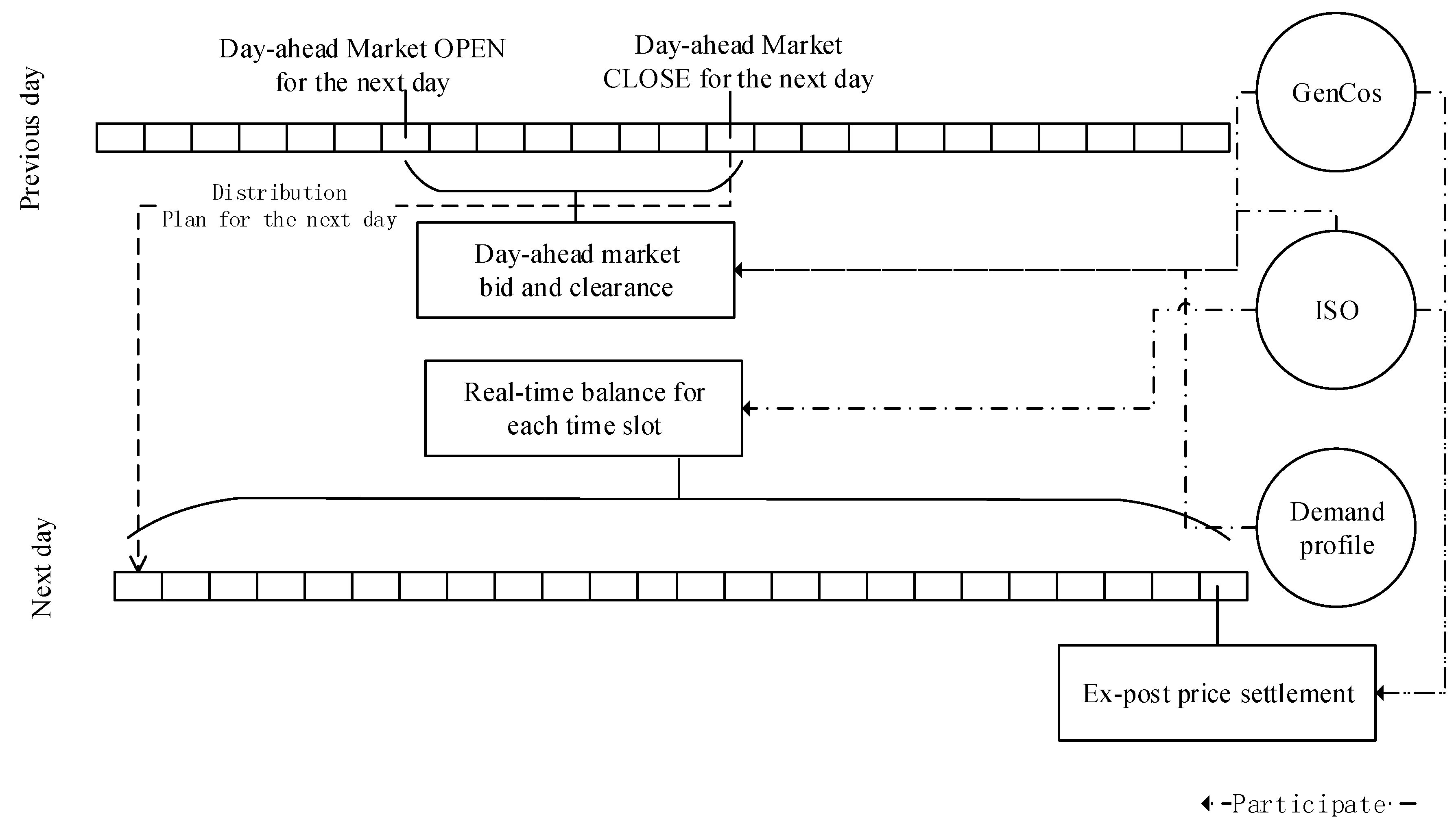
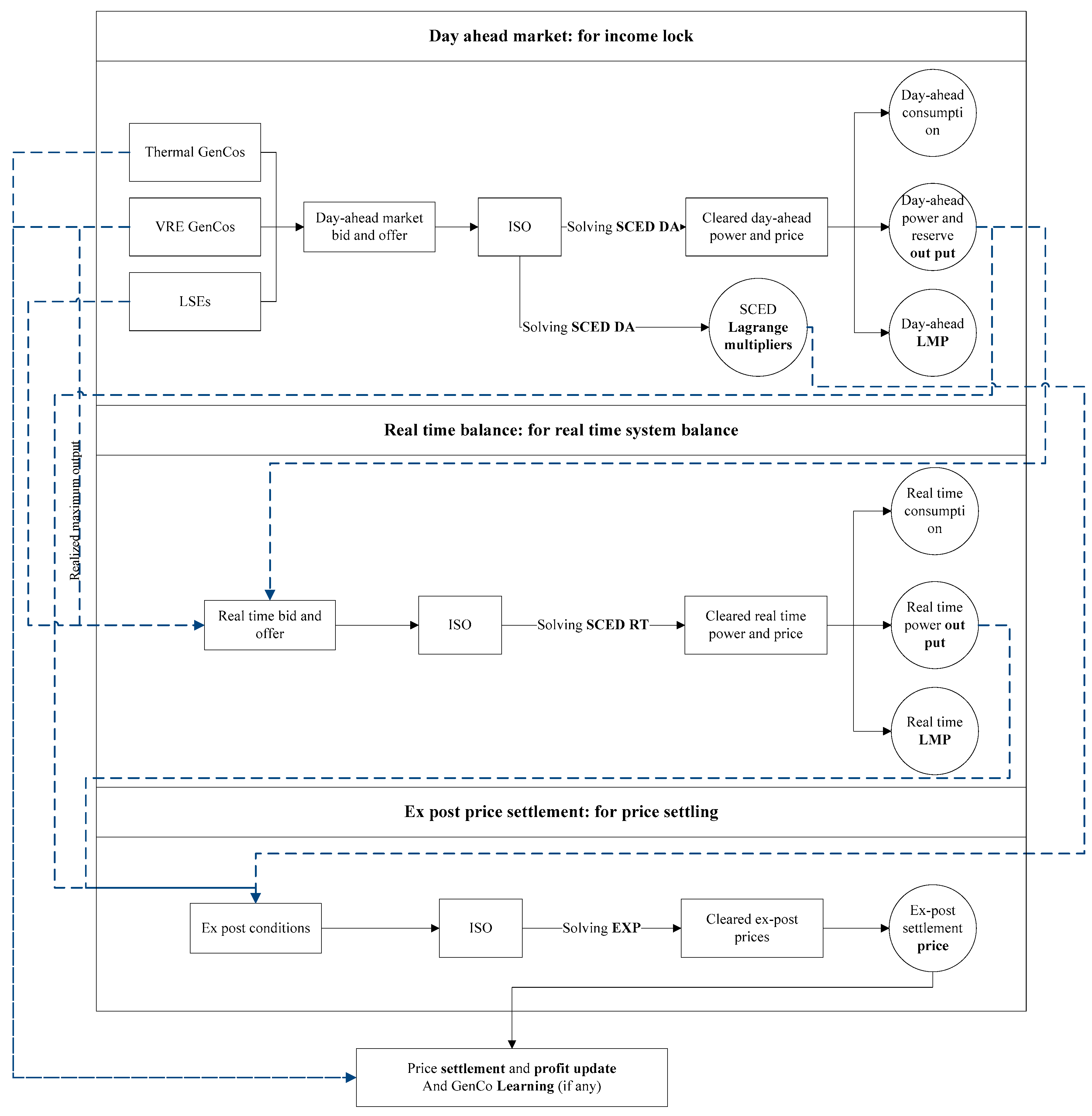
The brief market framework is illustrated in Figure 1. In the previous day, GenCos will bid in the day-ahead market. They will bid for both power and ancillary service. The day-ahead market opens at 6:00 and close at 15:00. ISO will clear the market for both power and ancillary service to acquire a dispatch plan. This plan will be carried out in the next day. ISO is responsible for keeping the system balanced for each time slot. It will dispatch reserves for this purpose. At the end of the execution day, ISO will carry out an ex-post settlement process. It will determine the settlement price for the market.
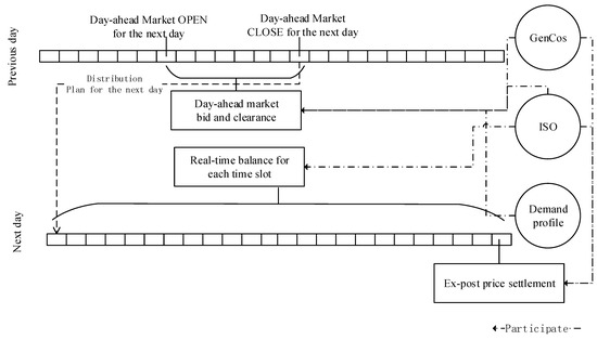
Figure 1.
Market framework.
Note that in this framework, energy demand is treated as a profile. This profile contains statistical forecasts of power loads in each system nodes. They are considered as given conditions in the calculation. In the model, they are represented by demand bids of load-serving entities. This treatment is common in energy system studies [10,17,47], when we want to focus on the influence of the supply side.
3. A VRE-Participated 2-Settlement Pool-Based Electricity Market
The short-term pool-based wholesale electricity market is more favorable for VRE than the long-term market because the accuracy of a short-term forecast is usually higher than the long-term one. Moreover, system security and ancillary service can be jointly cleared in the short-term market. In this paper, integration cost allocation is simulated by ex-post settlement and ancillary service clearing. Based on day-ahead clearance, optimal real-time and ex-post clearance can be carried out. Under a perfect market assumption (information is perfect and all participators act based on their true information), the system equilibrium can be reached by optimal clearing method. When learning and strategic behavior of GenCos are adopted, a more realistic influence result can be achieved [53,54,55]. Therefore, this paper builds a 2-settlement electricity-ancillary service conjugated market for VRE participation according to standard pool-market design.
3.1. Production Model of Thermal and VRE GenCos
In the model, the supply side is constituted by thermal and VRE GenCos (Generation Companies). It is assumed that a thermal GenCo has a quadratic form of production function. This is a widely applied assumption [56,57]. It is in the following form:
where is the production cost of a thermal GenCo. is the set of thermal GenCos. is the output of GenCo i. and are the coefficients of the production function.
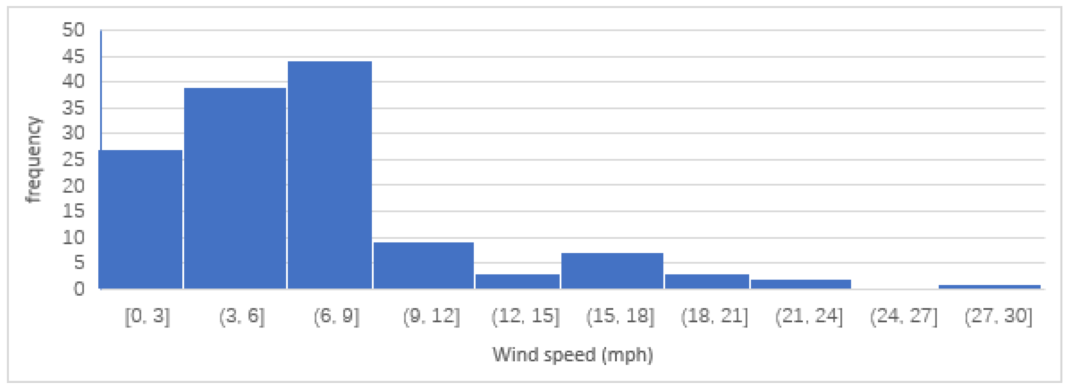
Wind power is a widely adopted variable renewable energy. The maximum output of a wind turbine is affected by the wind speed, which is a variable factor. Wind speed varies each hour. The wind speed distribution of an observation point in Beijing at 0:00 from 2018/1/1 to 2018/5/14 is shown in Figure 2. This is the basic property of variability of VRE. Output of VRE such as PV and wind are affected by many meteorological factors, such as temperature and wind speed [58,59].

Figure 2.
Wind speed at an observation point in Beijing at 0:00 from 2018/1/1 to 2018/5/14 [60].
Many researchers contribute to the field of VRE output forecast. Despite the differences in methodology, many of the studies show normal distribution patterns of forecast error [58,61,62]. Note that the wind speed or solar energy output may not necessarily comply with normal distribution. In fact, many observations show that they do not, such as the one in Figure 2.
Normally, VREs can be treated with 0 marginal production cost, so that VRE power output forecast cost becomes an important cost in short-term power market. This paper establishes an economic model to describe the relationship between output forecast error and forecast cost, since it can essentially affect the profitability of VREs in the short-term power market. As will be mentioned in Section 3.2, the error is the difference between the reported value and the realized output. So, forecast cost is essentially a reliability cost. There are many approaches to enhance the day-ahead reliability of a wind or solar power plant, such as adding investment in short-term wind power forecast, and in local energy ancillary sources such as storages.
In a day-ahead market, a VRE GenCo will forecast its next-day maximum output level for each hour, assuming to be . So, it can report a forecasted power generation limits to the Independent System Operator (ISO). Let us assume the forecast error range is , is the standard deviation of a normal distribution . The error complies with . The density of normal distribution is very low out of the range , so we assume .
In order to make the simulation results comparable, an important assumption is made. We assume that the marginal reliability cost function of a VRE GenCo is affine, same as the marginal production function of a thermal GenCo (this paper adopts quadratic form of production function). When a VRE GenCo is able to achieve an error level of at a reliability cost, the cost is in the following form:
where is the reliability cost for v. is the set of VRE GenCos. is the max capacity of v. and are the coefficients of the reliability function. is a pseudo-max-cost, which has the following value:
The setting of is just to make the mapping: . Note that
where Equation (4) is an affine function of . As we can see from Functions (2)–(4), this paper established an affine-first-order-derivative reliability cost function for the VRE GenCos, so that the first-order-derivatives of both VRE and thermal GenCos are affine. In fact, the reliability cost function can come in many forms, like exponential. However, the reliability cost function is affected by the reliability technology applied. This paper will not discuss the influences of this factor, although the model built by this paper gives a good framework for the discussion.
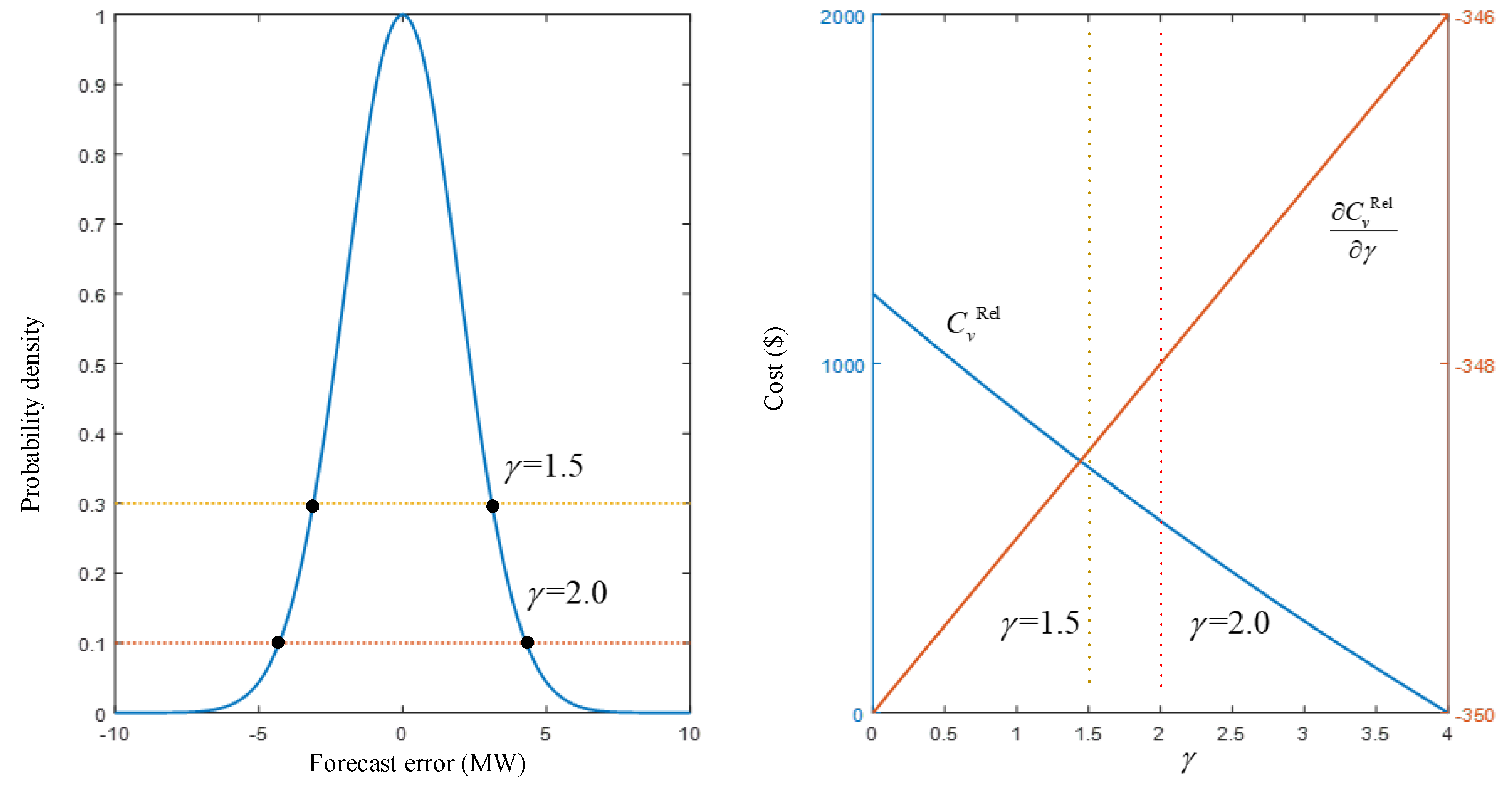
For example, if the parameters of a VRE GenCo is as shown in Table 1, the relation of reliability and cost is shown in Figure 3.

Table 1.
Parameters of a variable renewable energy (VRE) GenCo.
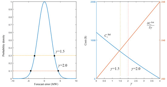
Figure 3.
The relationship between short-term reliability and forecast cost.
Note that parameters can be set to fit the practical situation. If a VRE GenCo does not control its forecast error, then and no reliability cost will occur. If a VRE GenCo increases cost in reliability control, for example in storage, then both fixed cost and variable cost will occur in reliability control. The variable cost is connected to the error range. Note that the first-order-derivative can be quite large when approaches 0, then the form of exponential function may be a better fit. However, in this paper, the variable reliability cost is assumed to be quadratic along with the production cost of thermal units.
If the operation of the market result in an amount of is cleared for (a VRE GenCo) to deliver, bears 2 types of risks: ① Its realized maximum power is lower than . This means negative deviation of power output happened, and has to bear deviation cost. ② Its realized maximum power is higher than . This means has to bear energy curtailment of .
3.2. Day-Ahead forward Market Considering Reserve Services for Variability
Inspired by the authors of [63], the day-ahead market is cleared by multi-period DC-OPF model for each hour in a day. VREs are allowed to participate in the market. This paper applies DC-OPF model because it is a simplified model while maintains accuracy when certain assumptions are satisfied. The simplicity helps unveiling the patterns of VRE market participation.
There are some basic settings and assumptions as follows.
Assumption 1.
The resistance for each branch is negligible compared to the reactance and can therefore be set to 0 [63].
Assumption 2.
The voltage magnitude at each node is equal to the base voltage [63].
Assumption 3.
The voltage angle difference across any branch is sufficiently small in magnitude [63].
Assumption 4.
Thermal GenCos and VRE GenCos can lock income in day-ahead market. The production function of thermal GenCos and reliability function of VRE GenCos have quadratic form, and their first-order derivatives have affine form.
Assumption 5.
The ISO will announce the reserve demand for imbalance for the intraday operation before the day-ahead market bidding.
Assumption 6.
No-load, start up and shut down cost of units are neglected. Thus, all units can be treated as committed and Security Constrained Unit Commitment (SCUC) problem solving would not be needed.
Assumption 7.
The ISO will solve a DC-OPF Security Constrained Economic Distribution (SCED) problem to for each hour of the next 24 h at the beginning of each day in the day-ahead clearing.
Assumption 8.
All GenCos are committed.
Assumptions 1–3 are to simplify the computation requirement. Assumptions 4–8 set a basic VRE-participated model of a day-ahead power market. The simplification will not ease the significance of the results and conclusions.
The day-ahead SCED problem (SCED DA) is as follows.
r.t.
s.t.
We have: , , , , , .
is the production function, for , for . is the production function for ancillary service, which is the reserve service in this problem. also has quadratic form . And the ancillary service can only be provided by thermal GenCos in this setting. is a penalty function to make sure Assumption 3 is satisfied.
Condition (5) considers the node active power balance. is the sum of demand bid by load-serving entities (LSE). is the sum of demand offered by GenCos including thermal and VRE GenCos. is the sum of power drawn from node k by the system. is the Lagrange multiplier of this condition.
Condition (6) considers the Ancillary service requirement. Based on Assumption 6, this paper only deals with short-term reserves. is a hourly reserve requirement proposed by the ISO, and considered as a control factor. It must not be smaller than the sum of reserve quantity offered by the thermal GenCos. It is related to the system balance, and to short-term reserve cost for VRE integration. Note that in a complex practical market, the ancillary service requirement is much more than a short-term requirement. It includes load following, regulation, long-term reserve, reactive compensation, frequency adjustment and so on.
Condition (7) considers the transmission line security constraint. is the maximum magnitude capacity of transmission line km.
Condition (8) claims that the sum of the active power offer and reserve offer cannot exceed the maximum generation capacity. Note that is reported by thermal GenCo.
Condition (9) is the lower output constraint of a VRE GenCo. Note that is reported by thermal GenCos.
Conditions (10) is the output constraint of a VRE GenCo. Note that and are reported by VRE GenCos.
Condition (11) is the value range constraints of variables.
In this model, the marginal generation cost of VRE is treated as 0. However, costs need to be paid if a VRE GenCo wants to maintain a certain level of generation reliability, as described in Section 3.1. But this cost is not considered by the ISO as part of the objective function. This is a reasonable consideration, because under current spot market mechanism, the production cost is quantity-based.
The day-ahead cleared ancillary service price is .
3.3. Real Time Balance
To simplify the model and make the mechanism trackable, we make another assumption here.
Assumption 9.
There is no intra-day sudden outage of a VRE generation unit or a thermal unit or a transmission line.
Assumption 9 means that the variability of active power output of VRE GenCos is the only uncertain factor in the model. By eliminating other uncertain factors, this setting helps analyze the influence of integration of VRE to the cost and efficiency.
The ISO will maintain the system balance by solving another real time SCED problem (SCED RT) as follows. For each real-time period:
r.t.
s.t.
We have: , , .
In real-time (every hour for simplification), the actual maximum output capacity of a VRE GenCo is realized. is the realized value.
is the penalty function for node load imbalance. We have:
Condition (12) is the real time node balance constraint. It is similar to Condition (15) while a slack variable is allowed. . and are recognized as “imbalance factors”, which is a measurement of the negative effect of the variability of VRE on the system. Based on and , the imbalance cost can be measured. Since the only uncertain factor is the output variation of VRE, the imbalance cost brought by VRE integration can be measured by and . is a penalty factor.
Condition (13) is real time transmission line security constraint.
Condition (14) is the real time output constraint of a thermal GenCo. The lower limit is consistent with the day-ahead report. The upper limit is the sum of cleared day-ahead cleared power output and reserve output.
Condition (15) is the real time output constraint of a VRE GenCo. The lower limit is consistent with the day-ahead report. The upper limit is the minimum of realized maximum output and day-ahead cleared power output.
Condition (16) is the value range constraints of variables.
From model SCED RT, we can see that the system is optimally dispatched based on the real time status of the system.
3.4. Ex-Post Settlement
Ex-post settlement is important for determining the cost of deviation. There are many researchers studying the ex-post settlement mechanism [64,65]. In this paper, we adopt the idea proposed by Zheng and Litvinov [66].
Under the assumption of perfect market and perfect information, from an ISO perspective, for each GenCo agent , in equilibrium, it faces the following profit maximization problem (PMP). For each period:
s.t.
. is the day ahead LMP, is the cleared day ahead reserve price.
The first-order KKT condition of this problem can be formulated as:
The complementarity conditions are:
and are Lagrange coefficients obtained by solving the SCED DA problem. According to the work of Zheng and Litvinov [66], if the result of the SCED DA problem can be treated as the equilibrium result of the day ahead situation, then the Karush-Kuhn-Tucker (KKT) condition of the PMP problem gives a good constraint for the ex-post settlement problem. In this paper, we ignored the Conditions (22)–(25), because the ex-post settlement condition is a deviation to the SCED DA result; additionally, we consider learning and strategic behavior for GenCos, then the Conditions (22)–(25) could be too strong and lead to problem infeasibility.
As a result, this paper set the ex-post settlement as the following problem (EXP). For each :
r.t.
s.t.
and (w belongs to node k). The solution and give the ex-post price.
and are Lagrange function imbalance factors. is a penalty factor.
Conditions (27) and (28) are respectively the Lagrange function of the active power maximization and reserve power maximization problem in PMP.
The settlement price is as follows:
is an ex-post settlement threshold, and . Condition (30) means that if the actual output deviates from the day-ahead cleared amount and the deviation exceeds a threshold, the ex-post price should be applied.
3.5. Learning and Strategic Behavior of GenCos
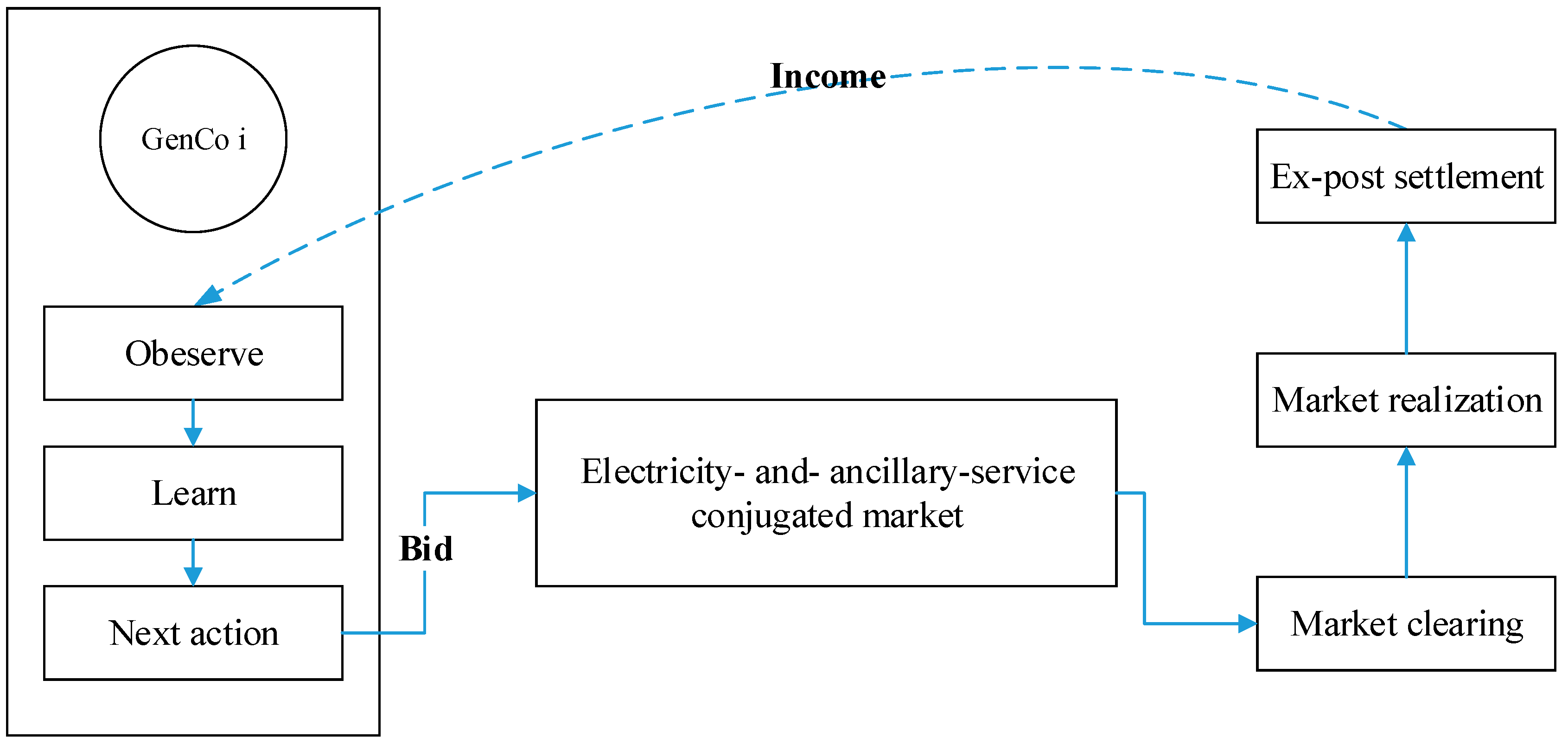
Ideally, GenCos report their true production parameters to the ISO. Under this situation, ISO can clear the market with true marginal condition and reach society optimality. However, there exists information asymmetry in the market. The true production parameters are private information of the GenCos. In the real world, market participators are humans. Human behavior is complicated. In the market, participators will observe the profit brought by their previous action and choose the best action (bid parameters) that brings the most income. This process can be simulated by reinforcement learning method. The process is illustrated in Figure 4.
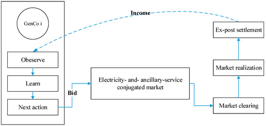
Figure 4.
Learning and strategic behavior of GenCos.
This paper considers strategic behaviors of GenCos. For each period, for a VRE GenCo at maximum output level , it can achieve a forecast error level at with mean value at a cost level of . However, can report strategic coefficients (, ) to the ISO, as a result of a learning process. Moreover, can learn to adopt a best value (reliability level) to a day’s operation.
Similarly, a thermal GenCo will learn to strategically report (, , , ) to the ISO in the day ahead market. This paper adopted the famous Erev–Roth reinforcement learning method to simulate the learning behavior of GenCos [67,68]. This method imitates the learning process of human being; thus, it grants us a chance to study the influences of learning and strategic behavior. Learning and strategic behavior make the system equilibrium hard to track, but it is a more practical setting than perfect market assumption. The consequences of learning and strategic behavior can be tracked by simulation approach as shown in this paper.
3.6. Case Design and Numerical Simulation
The case design principle is shown in Figure 5. Two scenarios are set to formulate comparison. Under one scenario, agents do not have learning and strategic behavior while under another scenario agents have learning and strategic behavior. The result comparison can show the influences of the learning and strategic behavior. This paper mainly considers three kinds of trackable integration costs, which are widely considered in practical VRE participated markets. Through the design of the 2-settlement electricity-ancillary service conjugated market in Section 3.1, Section 3.2, Section 3.3, Section 3.4 and Section 3.5, they can be simulated numerically. Ex-post settlement will determine deviation cost of VRE, since we rule out other deviations. Conjugate ancillary service clearing will show the cost of ancillary service. Since VRE are the only uncertainty source need for ancillary service, they must bear all the ancillary service cost. System imbalance cost is the cost of lost load. Since the total capacity is enough, load is lost because of the output uncertainty of the VRE.
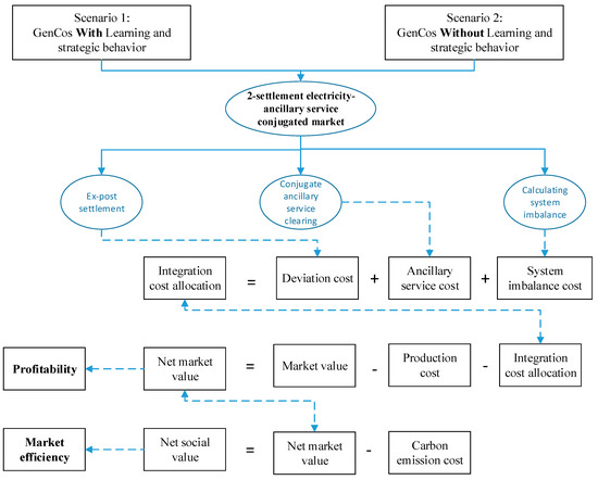
Figure 5.
The case design principle.
Profitability of VRE is characterized by their net market value, which is the net income of the VRE in the market. It equals market value minus production cost and minus integration cost. Market efficiency is characterized by the net market value of VRE. It characterized the net benefit the VRE brought to the society.
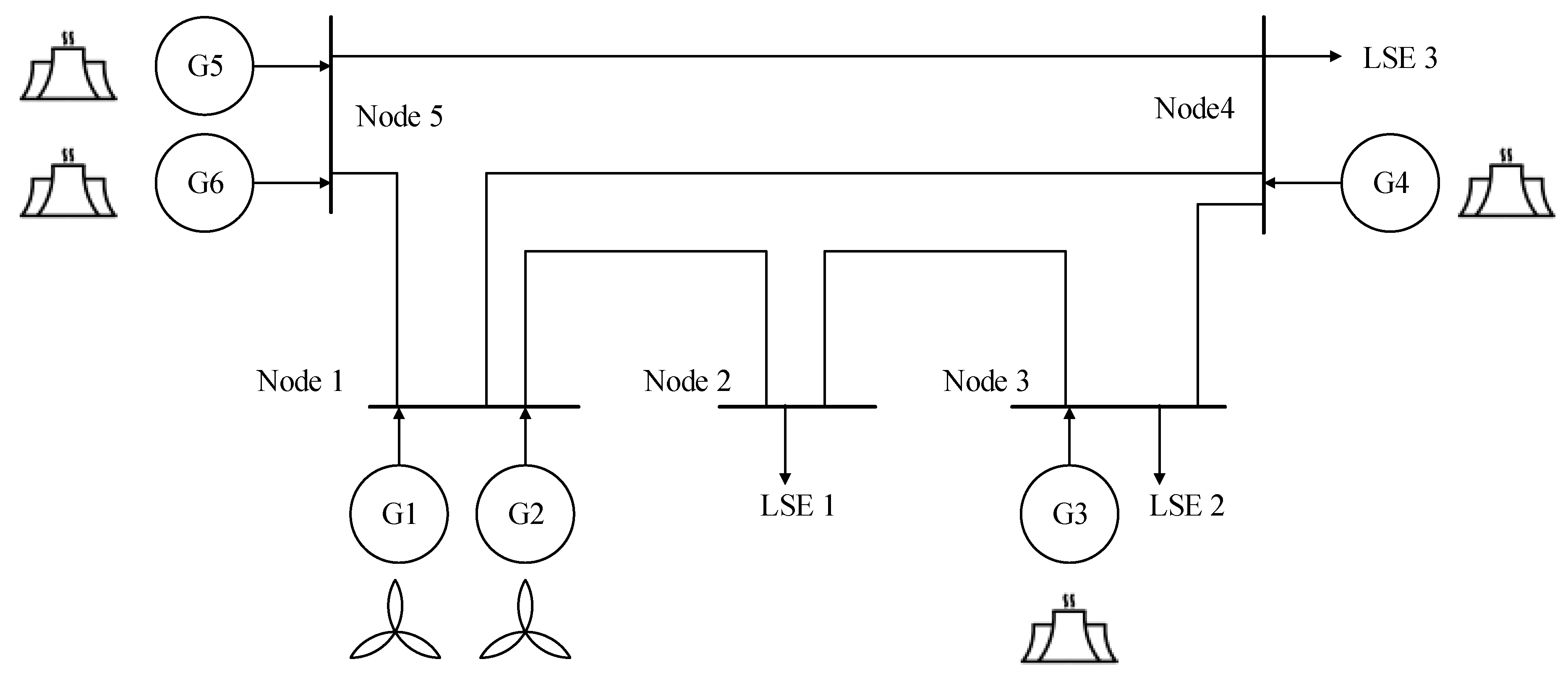
This paper extended the standard 5-node test framework in the work of Sun and Tesfatsion, and Li and Tesfatsion [63,69]. The system structure is shown in Figure 6. There are 6 GenCos and 3 load-serving entities (LSEs). G1 and G2 are VRE GenCos, and the others are thermal GenCos. Initial properties of GenCos are shown in Table 2. The transmission line properties are shown in Table 3. All the parameter explanation can be found in the Nomenclatures table at the front of this paper.
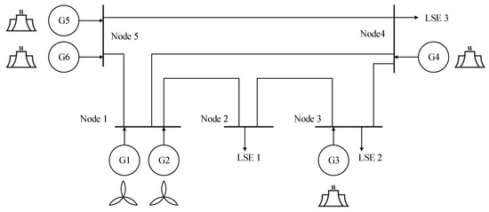
Figure 6.
A five-node test framework.

Table 2.
Initial properties of GenCos.

Table 3.
Transmission line properties.
The parameter setting is representative. Note that in Table 2, the reserve cost coefficients are 1/10 of the production coefficients, because reserve cost is usually the no-load cost of the unit. It is significantly smaller than the production cost. For VRE GenCos, GenCo1 and GenCo2 have the same fixed cost, initial money and learning settings. The installed capacity ratio of VRE GenCo is 13.16%. This ratio is representative, because it is nearly the practical ratio of many countries (except for some wind dominant countries such as north European countries).
The simulation process can be found in Figure 7. At the beginning of the day-ahead market, LSEs provide their load profile to the ISO. To make the result trackable, this paper does not consider price-sensitive bidding and strategic behavior of the LSEs. In other words, all demands are price-inelastic. This paper adopt the 24-h load profile in the work of Sun and Tesfatsion, and Li and Tesfatsion [63,69]. To eliminate the influences of load variation between days, the load profile is the same for each day.
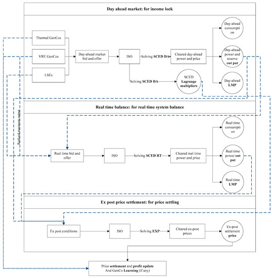
Figure 7.
The simulation process.
This research carried out two scenarios of test cases, all of which lasted for 30 simulation days. The condition variation is shown in Table 4. Note that when reserve level is 0 MW, there are no ancillary services for VRE. This will expose the negative influences of the variability of the VRE GenCos. When the reserve level is 200 MW, it covers all of the VRE capacity. Note that when GenCos do not have learning ability, they bid by their true parameter value, and thus the system operation result can be treated as an equilibrium result.

Table 4.
Test case settings.
4. Results and Discussion
4.1. Profitability of VRE
Market values are calculated as follows:
Market value of GenCo w is the weighted average of the LMP and ancillary service price.
Based on cost-causation principle, the integration cost should be calculated for the net market value of VRE. To acquire the net market value, production cost and integration cost are considered. Net earnings are calculated as follows:
. is the net earnings of GenCo w.
and are node imbalance factors. We assume imbalance cost can be measured, as follows:
is an imbalance measurement factor. .
Let us assume , which means imbalance unit cost is 1 times the LMP of a node.
Reserve cost of the system is as follows:
The net market value of a GenCo is as follows:
is the net market value of GenCo w. means the imbalance cost allocated to w. means the ancillary service cost allocated to w. In the simulation cases, ancillary service cost is allocated based on installed capacity of VRE. So, it is evenly allocated between the 2 VRE GenCos.
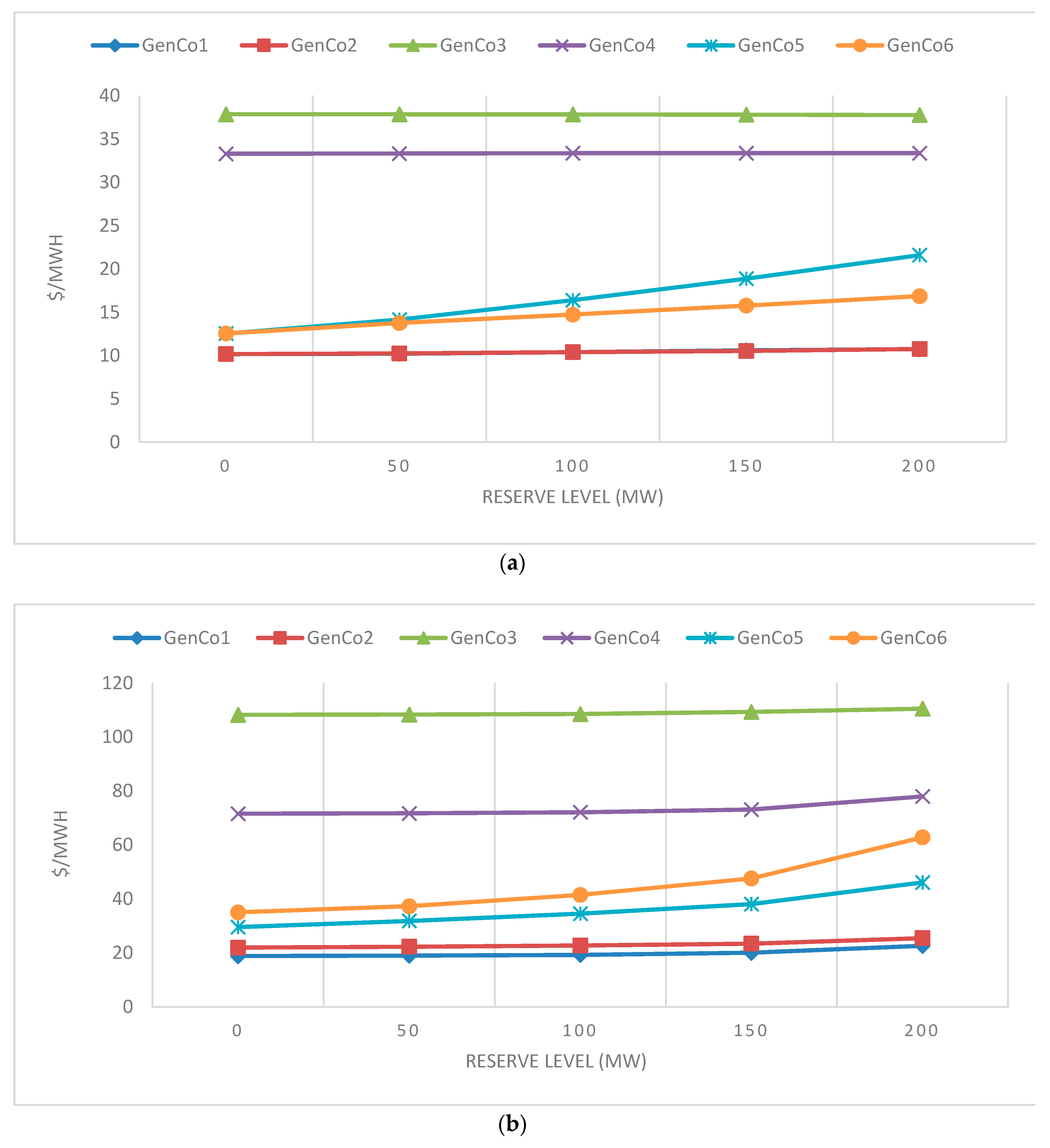
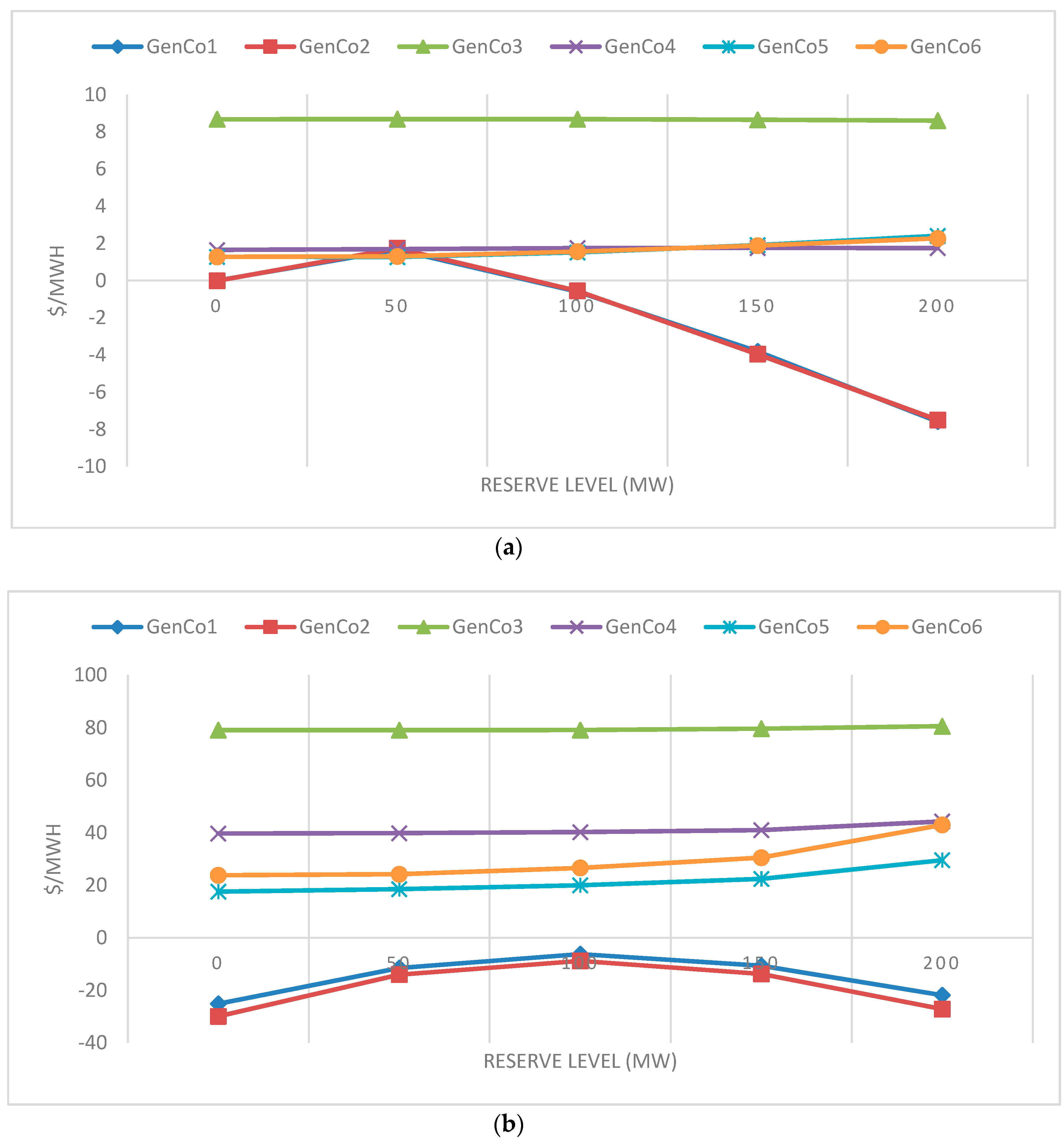
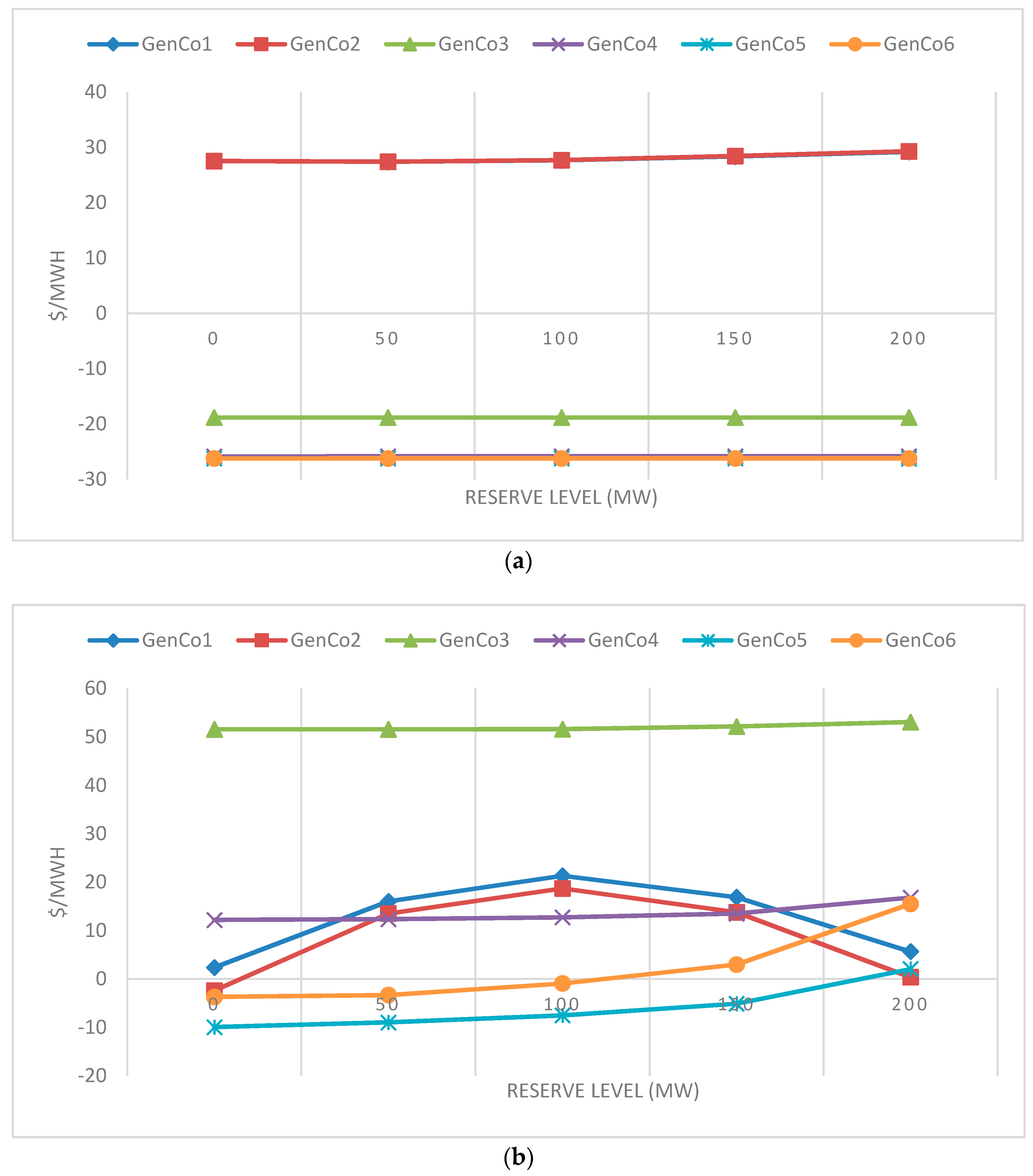
Note that this calculation ignored reduction of full-load hour (RFH) and grid cost mentioned in Section 2 because they are somehow hard to track and not included in the model. For overproduction cost, it can be measured in the simulation as the curtailment cost. However, the author believes that it is not proper to add it as a cost for a VRE GenCo. Because the value of curtailment is more understandable in conventional FiT or RPS mechanisms. In the market, the curtailment is just a risk for a VRE participator. The market values and net market values of GenCos in each equilibrium case can be seen in Figure 8a and Figure 9a. The market values and net market values of GenCos in each learning cases can be seen in Figure 8b and Figure 9b.
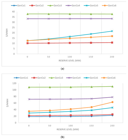
Figure 8.
(a) Market value of GenCos without learning and strategic behavior. (b) Market value of GenCos with learning and strategic behavior.
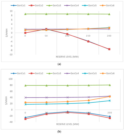
Figure 9.
(a) Net market value of GenCos without learning and strategic behavior. (b) Net market value of GenCos with learning and strategic behavior.
By comparing Figure 8a,b, we can see that the market value of GenCo5 and GenCo6 tend to increase with reserve level. This is because the reserve service is mainly provided by GenCo5 and GenCo6, as an outcoming of ancillary service clearing. We can also see that market values of all GenCos enjoy a great uplift when learning and strategic behavior is adopted. This shows the fact that consumer surplus is consumed by the strategic behavior of the GenCos. We can also see that the market values of VRE GenCos (GenCo1 and GenCo 2) are the lowest among all the GenCos.
When we look at the net market value, we find that the profitability of VRE GenCos is unoptimistic. Under almost all cases, VRE has negative net market value, except for the no learning cases where reserve level is low. While thermal GenCos managed to uplift their net market value by a great deal by learning and strategic bidding, the net market value of VRE get a decrease when learning and strategic behavior is applied. This shows a great disadvantage for VREs in pool-based market.
We show the market value and net market value of VRE GenCos in no learning cases by (reliability of VRE) level in Figure 10a,b.
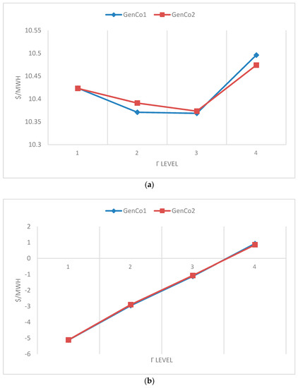
Figure 10.
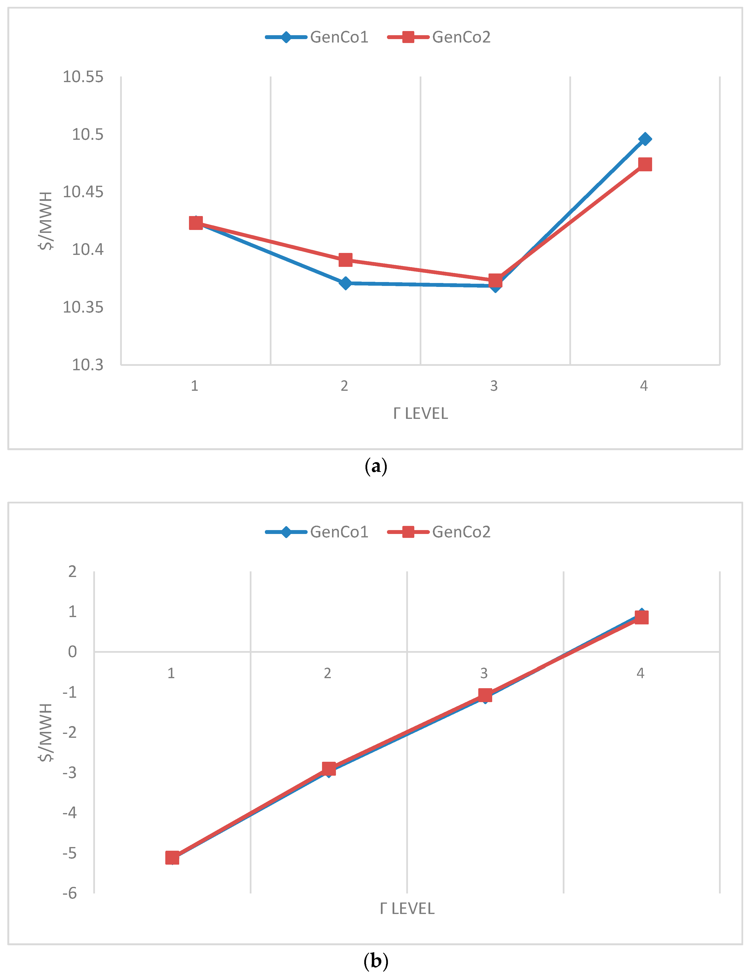
(a) Market value of GenCos without learning and strategic behavior by . (b) Net market value of GenCos with learning and strategic behavior by .
We can see that from the perspective of market value in no learning cases, reliability shows little influence on the market value. From the perspective of net market value, not to maintain high reliability is definitely a better strategy for VRE GenCos. This is because the cost of maintaining high reliability is greater than the benefit of it for the VRE GenCos (in the simulation setting).
4.2. Efficiency of VRE in Market
The net social value of a GenCo is the profit it brings to the society minus the cost it brings. In this paper, it is calculated as follows:
. is the net society value of VRE GenCo v. is the carbon emission cost caused by w. Apparently, for thermal GenCos, it is a positive number while for VRE GenCos, it is negative.
where is the carbon price. (ton/MWh) is the carbon emission by unit power produced. is the power produced. The base values are chosen as: = 27.60 $/ton [70], = 0.997 ton/MWh. The net social value is shown in Figure 11a,b.
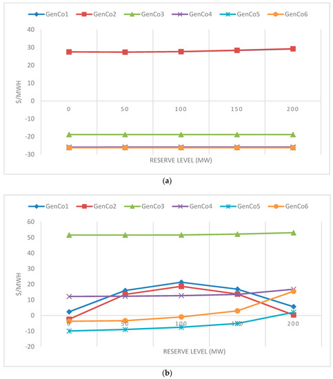
Figure 11.
(a) Net social value of GenCos without learning and strategic behavior. (b) Net social value of GenCos with learning and strategic behavior.
From Figure 11a, we can see that in no-learning cases reserve levels barely influence the net social value of GenCos, and that the net social value of VRE is much higher than that of thermal GenCos. However, we can find in Figure 11b, the net social value of VRE GenCos is somehow comparable to that of thermal GenCos. Thermal GenCo 3 has the highest net social value, because it managed to acquire a very high net market value by strategic bidding.
To study the influence of carbon price. The sensitivity analysis of net social value to carbon price is carried out. The result is shown in Figure 12a,b.
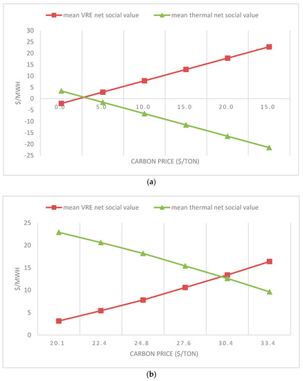
Figure 12.
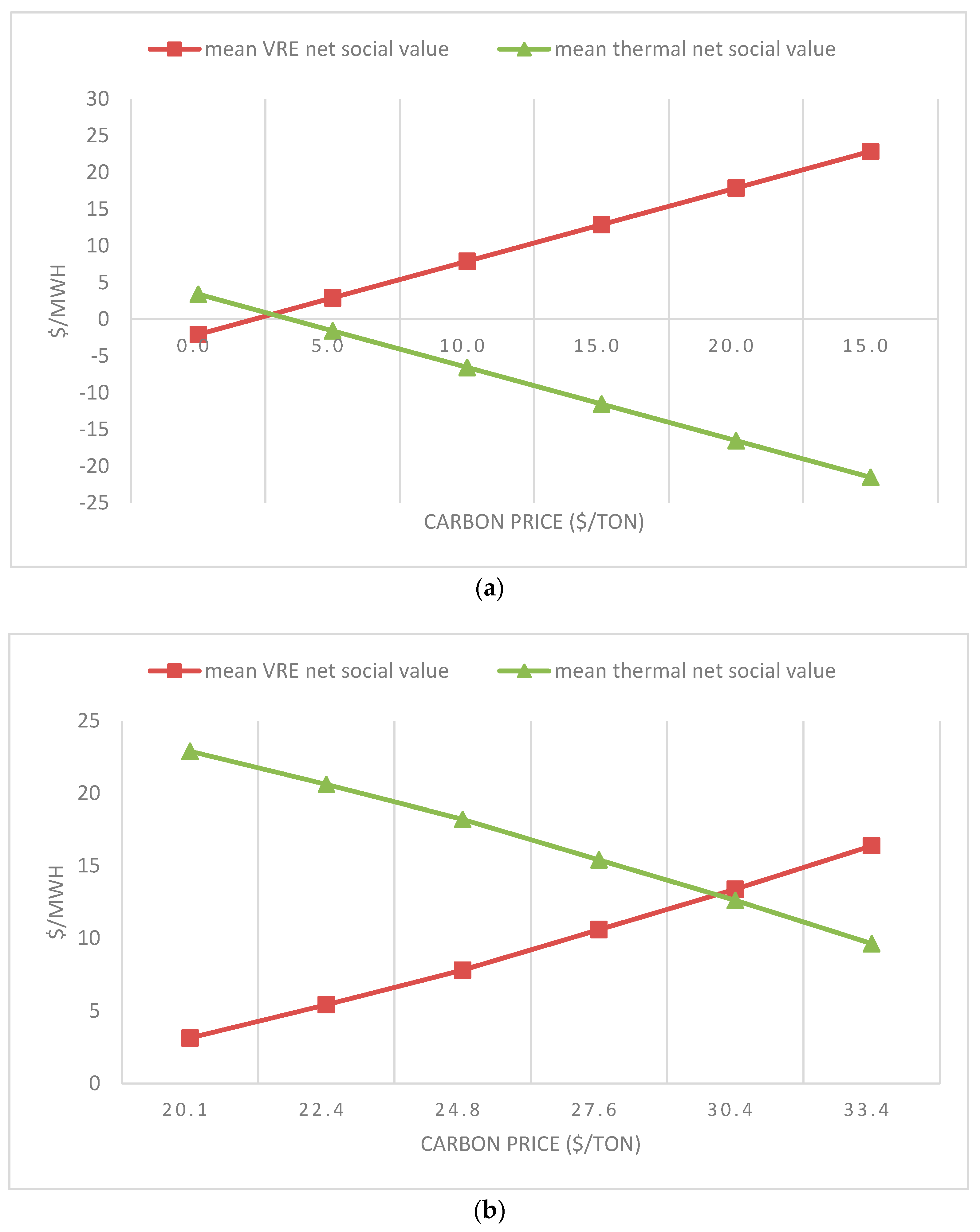
(a) Sensitivity analysis of net social value to carbon price without learning and strategic behavior. (b) Sensitivity analysis of net social value to carbon price with learning and strategic behavior.
By comparing Figure 12a,b, we can see that generally, the net social value of VRE increases as the carbon price increases, while the net social value of thermal units decreases as the carbon price increases. We define the carbon price where net social value of VRE and thermal as balance point. At the balance point, VRE units bring just as much of the net social value as that of thermal units. We can see that learning and strategic market behavior can essentially uplift the balance point. This means that if the market mechanism cannot rule out strategic bidding, the carbon price where VRE can act as a truly “better” energy source can be high.
4.3. Discussions
4.3.1. Locational Marginal Price of VRE
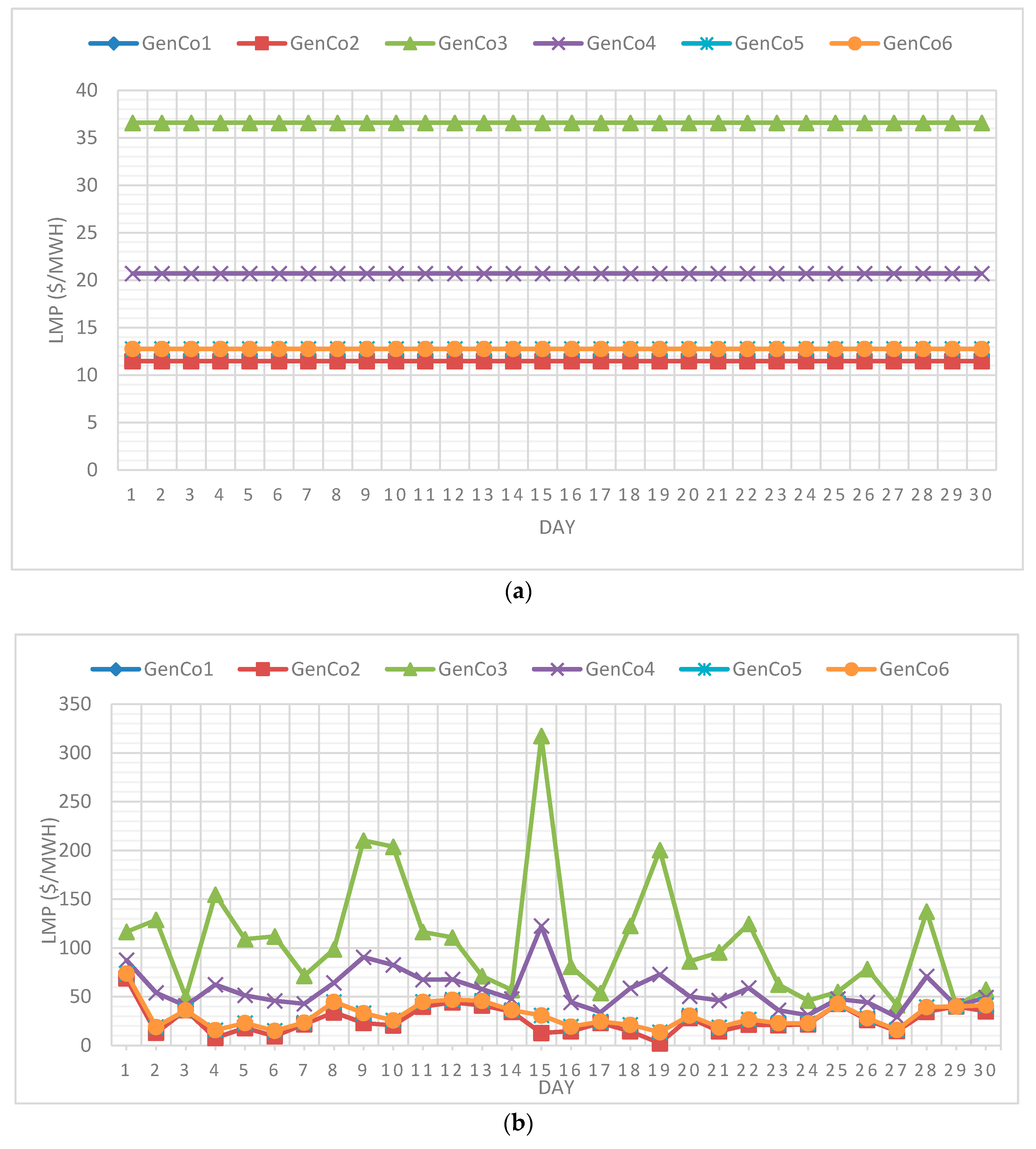
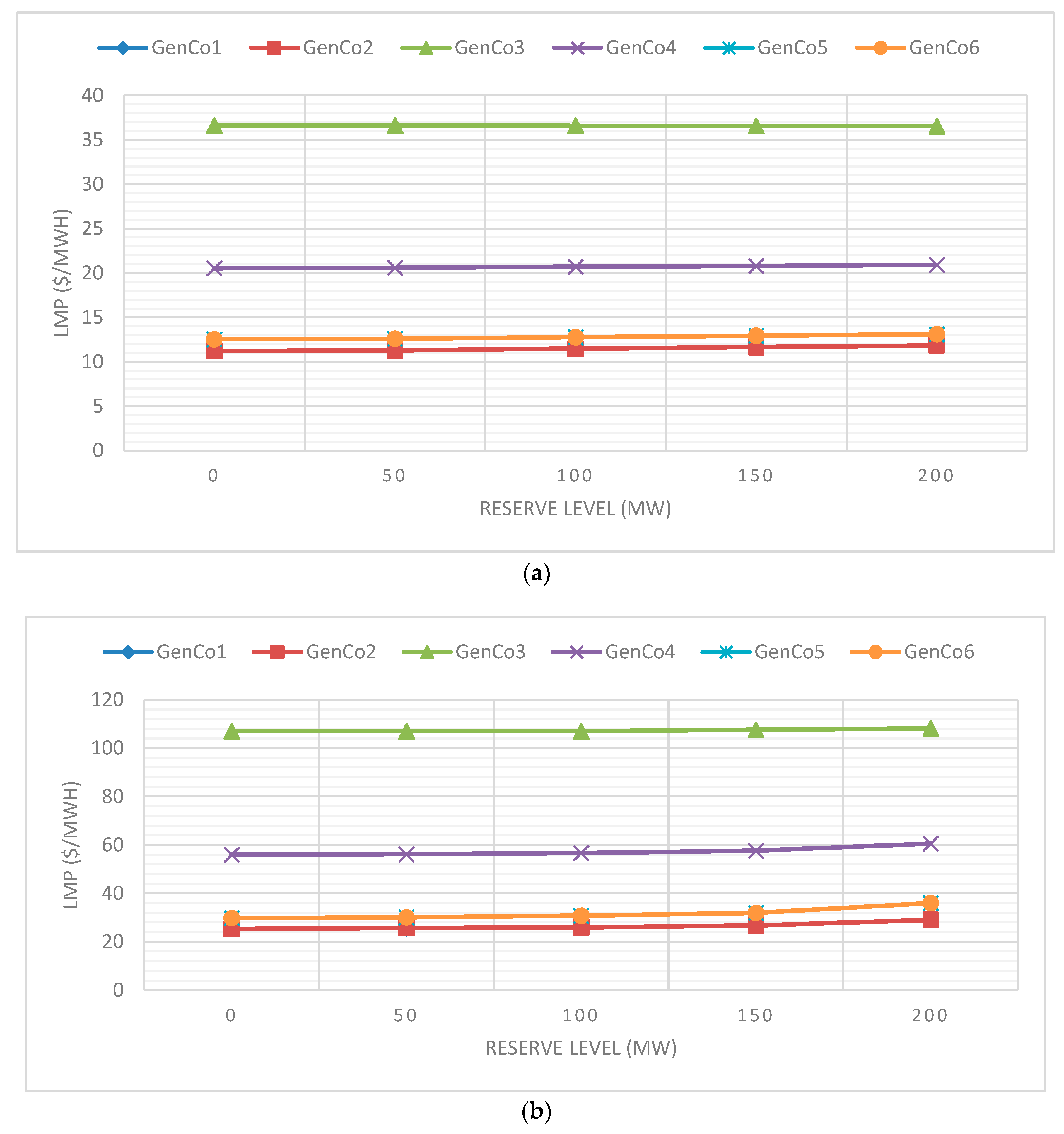
In this section, we try to determine the reason of low profitability of VRE in pool-based market. Under standard pool-based 2-settlement market mechanism, price volatility varies much between no-learning and learning cases. Compare Figure 13a,b, we can see that since GenCos always submit their true parameters, Locational marginal price (LMP) does not vary in the no-learning case (note that the influence of load is eliminated), while LMP varies much in the learning case. As can be seen in Figure 14a,b, in both no-learning and learning cases, the system reserve level shows little influence on the LMP.
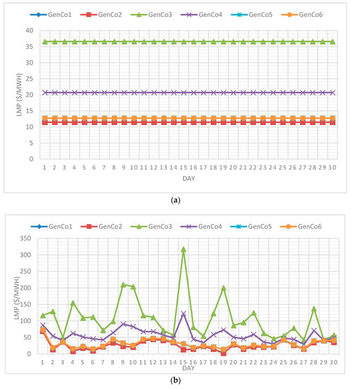
Figure 13.
(a) No-learning case, reserve level = 100 MW, = 2. (b) Leaning case, reserve level = 100 MW.
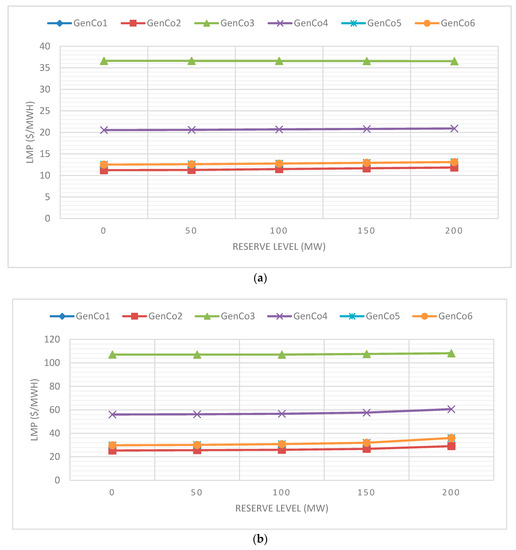
Figure 14.
(a) Average LMP level in no-learning cases under different system reserve levels. (b) Average LMP level in learning cases under different system reserve levels.
By comparing Figure 14a,b, we can see that the average LMP in the learning cases is much higher than that in the no-learning cases. Meanwhile, the LMP of VRE is always lower than that of the thermal GenCos. This paper gives a theoretic analysis as follows, to prove that the LMP of VRE nodes will always be lower than that of pure thermal nodes. We call this phenomenon the LMP disadvantage of VRE.
The production cost of a VRE plant has the following property: The production is dependent on nature force. For example, a PV plant output is dependent on the solar radiation. Thus, this paper makes the assumption: the variable production cost directly related to power generation is far less than conventional power plants which consume fuels, no matter what the production quantity is. This phenomenon can be expressed in the following formulation:
For a standard DC-OPF security constrained economic dispatch (SCED) problem:
r.t.
s.t.
where is the load demand at node k; is the power generated at node k; is the power withdrawn from node k; is the power flow in line km (from node k to node m).
Based on the work of Caramanis [71], the Locational Marginal Price (LMP) of node k is:
To analyze the LMP for VRE plants in the system, this paper makes some assumptions. This paper wants to eliminate the influence of line capacity. Firstly, it is assumed that the lower and upper bounds of line capacity constraints are not binding. This means assuming the transmission line capacity is large enough and . Secondly, it is assumed that the DC-OPF SCED problem is convex. Under the assumptions, let us look at the Lagrange function of KKT condition of the DC-OPF SCED problem.
where is the LMP in node k.
For the wth component in Equation (43), we have:
where means that GenCo w is in node k. and .
From Equation (44), we can get the value of :
where is the quantity for GenCos in node k.
It can be proved that when and , . stands for a minor change. The proof can be found in Appendix A.
From the following analysis we can see that VRE GenCos always have LMP disadvantage in DC-OPF SCED clearance.
For a , the expression reaches the maximum value when . It happens when VRE GenCo reaches its upper capacity bound in the clearance. The maximum value is . Based on Equation (32), we have:
Suppose . We always have:
Note that .
Thus, we can draw the following conclusion:
, if there are more VRE GenCos in node k1 than k2. .
What is the influence of LMP disadvantage? It drives down the LMP of VRE node in the system, which is a phenomenon observed in reality [44,46,72]. Low LMP means low income. Although the production cost of VRE is very low, VRE GenCos must bear integration costs. If VRE wants to strengthen reliability, it must increase reliability cost. All these factors will drive down the profitability of VRE in a pool-based power market.
4.3.2. The Market Value and LCOE of VRE
Traditional FiT mechanisms only focus on the price of VRE generated unit power. FiT is usually based on the LCOE of a specific kind of VRE [31,33,35]. FiT is imposed to ensure the unit power price of VRE is higher or equal to the LCOE. To bring VRE to market, some pricing mechanism are proposed based on FiT and market value. Market premium mechanism is proposed in Germany to promote VRE market participation [43]. It ensures that the market value of VRE is not less than FiT. If so, it will be subsidized. However, as can be observed in Figure 8a,b, based on the LMP disadvantage phenomenon, the market value of VRE GenCos are much lower than the thermal GenCos. The LCOEs of some energy projects in United States and China are shown in Table 5.

Table 5.
The LCOE of some energy projects in United States and China [14].
We can see that the LCOE of some mature VRE technology like onshore wind and large-grounded PV is lower than traditional thermal power such as Ultra-supercritical coal and CCGT. Based on these data, some may conclude that VRE is profitable in pool-based market. Indeed, as a simulation result of this research, the market value of VRE in Figure 8a,b is somewhat acceptable comparing with data in Table 5. However, if integration cost is properly allocated, VRE will become unprofitable (net market value lower than LCOE). Learning and strategic market behavior will even weaken the profitability.
5. Conclusions and Suggestions
Based on the results and analyses of this paper, the following conclusions can be drawn.
LMP disadvantage hampers the profitability of VREs. LMP disadvantage roots in the low output-based marginal production cost in market clearing. Insufficient net market value will lead to pay-back period of VRE projects that is too long to be feasible. Thus, hampering VRE investment. Current market mechanism may be incentive incompatible for VREs. If we want to get positive net market value for VRE and market, we should consider the following approaches.
First, consider reliability cost of VRE in object function in pool-based market clearing. For example, VRE may be allowed to submit a reliability control cost function to ISO. Nevertheless, new mechanisms like deviation pricing should also be studied. The new mechanism should somehow be related to stochastic functions and optimizations, which puts a challenge in building VRE-participated pool-based power market.
Second, incomes from emission market constitute an important source of income for VRE GenCos. As we can see in Section 4.2, the higher the carbon price, the more profitable the VRE units. However, learning and strategic behavior in the electricity market will significantly weaken this advantage.
Third, Learning and strategic behavior is unneglectable in reality. It can make the market clearance result unforeseeable and unstable, and it should be restricted.
Two improvements can be made based on this work for future studies.
The time slot in this paper is relatively long. If big data of VRE source and demand can be acquired, more intelligent dispatch method may be applied based on shorter time slot to further promote VRE penetration.
This paper considers VRE marginal production cost as 0. This is true for some real markets. But in some markets, VRE may also submit none-zero cost coefficients. This situation may be further studied.
Author Contributions
Conceptualization, R.X.; Methodology, R.X. and Z.L.; Software, R.X.; Validation, Z.Y.
Funding
This paper is supported by the National Natural Science Foundation of China (Grant No. 71803046), the Research Funds of Beijing Social Science (No.16GLC069), the Fundamental Research Funds for the Central Universities (NO. 2018ZD14).
Conflicts of Interest
The authors declare no conflict of interest.
Abbreviations
| Rel | Reliability |
| pse | pseudo-max-cost |
| H | Upper limit for GenCo output |
| L | Lower limit for GenCo output |
| U | Upper limit for transmission line capacity |
| Hr | Realized Upper limit for a VRE GenCo |
| AS | Ancillary service |
| rep | Reported value |
| DA | Day ahead values |
| RT | Real time values |
| Exp | Ex-post values |
| Set | Settlement values |
| O | Operation |
| Subindices and superindices | |
| i,v,w | Subindices for GenCos |
| k,m | Subindices for nodes |
| km | Subindices for a transmission line from k to m |
| l | Subindices for transmission lines |
| P, Q | Subindices for conditions in SCED DA |
| j | Subindices for load-serving entities |
| t | Subindices for periods |
| Constants and variables | |
| Forecast error factor for VRE GenCos | |
| Active power output for a CenCo | |
| Reserve power for a thermal CenCo | |
| Reactance of line km | |
| Power flow | |
| Voltage angle | |
| , , | Lagrange multipliers |
| Penalty factor | |
| Locational marginal price (LMP) | |
| Day ahead ancillary service price | |
| Load demand of active power | |
| Price imbalance factor | |
| A, B, C, D | Cost coefficients |
| M | Market power |
| Ex-post settlement coefficients | |
| Settlement price | |
| Imbalance measurement factor | |
| Sets | |
| I | Set of thermal GenCos |
| V | Set of VRE GenCos |
| BR | Set of VRE transmission lines |
| J | Set of LSEs |
| N | Set of Nodes |
| Set of periods | |
| Functions | |
| Production function for a GenCo | |
| Ancillary service production function | |
| A penalty function | |
| A penalty function | |
| Operators | |
| Absolute value or set cardinality |
Appendix A
Consider an optimization problem as follows.
s.t.
Suppose the dimension of , and are respectively , and .
The KKT of this problem is:
For ith dimension (), we have:
Suppose is the solution of the problem.
The first order Taylor approximation of at is:
So we have:
Combine Conditions (b) and (d), we have:
Suppose and , , , , . we have:
References
- Sawin, J.L.; Sverrisson, F.; Seyboth, K.; Adib, R.; Murdock, H.E.; Lins, C.; Edwards, I.; Hullin, M.; Nguyen, L.H.; Prillianto, S.S. Renewables 2017 Global Status Report; REN21: Paris, France, 2017. [Google Scholar]
- Shen, J.; Luo, C. Overall review of renewable energy subsidy policies in China–Contradictions of intentions and effects. Renew. Sustain. Energy Rev. 2015, 41, 1478–1488. [Google Scholar] [CrossRef]
- Kalkuhl, M.; Edenhofer, O.; Lessmann, K. Renewable energy subsidies: Second-best policy or fatal aberration for mitigation? Resour. Energy Econ. 2013, 35, 217–234. [Google Scholar] [CrossRef]
- Li, C.; Shi, H.; Cao, Y.; Wang, J.; Kuang, Y.; Tan, Y.; Wei, J. Comprehensive review of renewable energy curtailment and avoidance: A specific example in China. Renew. Sustain. Energy Rev. 2015, 41, 1067–1079. [Google Scholar] [CrossRef]
- Kane, L.; Ault, G. A review and analysis of renewable energy curtailment schemes and Principles of Access: Transitioning towards business as usual. Energy Policy 2014, 72, 67–77. [Google Scholar] [CrossRef]
- Fink, S.; Mudd, C.; Porter, K.; Morgenstern, B. Wind Energy Curtailment Case Studies: May 2008–May 2009; National Renewable Energy Laboratory (NREL): Golden, CO, USA, 2009. [Google Scholar]
- Denholm, P. Energy storage to reduce renewable energy curtailment. In Proceedings of the 2012 IEEE Power and Energy Society General Meeting, San Diego, CA, USA, 22–26 July 2012; pp. 1–4. [Google Scholar]
- Hirth, L.; Ueckerdt, F.; Edenhofer, O. Integration costs revisited–An economic framework for wind and solar variability. Renew. Energy 2015, 74, 925–939. [Google Scholar] [CrossRef]
- Milligan, M.; Kirby, B. Calculating Wind Integration Costs: Separating Wind Energy Value from Integration Cost Impacts; National Renewable Energy Laboratory (NREL): Golden, CO, USA, 2009. [Google Scholar]
- Koraki, D.; Strunz, K. Wind and solar power integration in electricity markets and distribution networks through service-centric virtual power plants. IEEE Trans. Power Syst. 2018, 33, 473–485. [Google Scholar] [CrossRef]
- Dragoon, K.; Milligan, M. Assessing Wind Integration Costs with Dispatch Models: A Case Study of PacifiCorp; Preprint; National Renewable Energy Laboratory (NREL): Golden, CO, USA, 2003. [Google Scholar]
- Ouyang, X.; Lin, B. Levelized cost of electricity (LCOE) of renewable energies and required subsidies in China. Energy Policy 2014, 70, 64–73. [Google Scholar] [CrossRef]
- Branker, K.; Pathak, M.; Pearce, J.M. A review of solar photovoltaic levelized cost of electricity. Renew. Sustain. Energy Rev. 2011, 15, 4470–4482. [Google Scholar] [CrossRef]
- IEA. Projected Costs of Generating Electricity; International Energy Agency (IEA): Paris, France, 2015. [Google Scholar]
- Bitar, E.Y.; Rajagopal, R.; Khargonekar, P.P.; Poolla, K.; Varaiya, P. Bringing wind energy to market. IEEE Trans. Power Syst. 2012, 27, 1225–1235. [Google Scholar] [CrossRef]
- Traber, T.; Kemfert, C. Gone with the wind?—Electricity market prices and incentives to invest in thermal power plants under increasing wind energy supply. Energy Econ. 2011, 33, 249–256. [Google Scholar] [CrossRef]
- Shin, H.; Baldick, R. Mitigating market risk for wind power providers via financial risk exchange. Energy Econ. 2018, 71, 344–358. [Google Scholar] [CrossRef]
- Lin, W.; Bitar, E. Forward electricity markets with uncertain supply: Cost sharing and efficiency loss. In Proceedings of the 2014 IEEE 53rd Annual Conference on Decision and Control (CDC), Los Angeles, CA, USA, 15–17 December 2014; pp. 1707–1713. [Google Scholar]
- Kirby, B.; Milligan, M.; Wan, Y. Cost-Causation-Based Tariffs for Wind Ancillary Service Impacts; National Renewable Energy Laboratory (NREL): Golden, CO, USA, 2006. [Google Scholar]
- Sotkiewicz, P.M.; Vignolo, J.M. Towards a Cost Causation-Based Tariff for Distribution Networks With DG. IEEE Trans. Power Syst. 2007, 22, 1051–1060. [Google Scholar] [CrossRef]
- Chakraborty, P.; Baeyens, E.; Khargonekar, P.P. Cost Causation Based Allocations of Costs for Market Integration of Renewable Energy. IEEE Trans. Power Syst. 2017, 33, 70–83. [Google Scholar] [CrossRef]
- Baeyens, E.; Bitar, E.Y.; Khargonekar, P.P.; Poolla, K. Coalitional aggregation of wind power. IEEE Trans. Power Syst. 2013, 28, 3774–3784. [Google Scholar] [CrossRef]
- Hernández-Moro, J.; Martínez-Duart, J.M. Analytical model for solar PV and CSP electricity costs: Present LCOE values and their future evolution. Renew. Sustain. Energy Rev. 2013, 20, 119–132. [Google Scholar] [CrossRef]
- Liu, Z.; Zhang, W.; Zhao, C.; Yuan, J. The Economics of Wind Power in China and Policy Implications. Energies 2015, 8, 1529–1546. [Google Scholar] [CrossRef]
- Yuan, J.; Sun, S.; Zhang, W.; Xiong, M. The economy of distributed PV in China. Energy 2014, 78, 939–949. [Google Scholar] [CrossRef]
- Xyu, R.; Song, Z.; Tang, Q.; Yu, Z. The cost and marketability of renewable energy after power market reform in China: A review. J. Clean. Prod. 2018, 204, 409–424. [Google Scholar]
- Yang, M.; Bewley, R. Integration of Variable Generation, Cost-Causation, and Integration Costs. Electr. J. 2011, 24, 51–63. [Google Scholar]
- Holttinen, H.; Meibom, P.; Orths, A.; O’Malley, M.; Ummels, B.; Tande, J.O.; Estanqueiro, A.; Gomez, E.; Smith, J.C.; Ela, E. Impacts of large amounts of wind power on design and operation of power systems, results of IEA collaboration. In Proceedings of the European Wind Energy Conference & Exhibition 2008, Brussels, Belgium, 31 March–3 April 2008. [Google Scholar]
- Ueckerdt, F.; Hirth, L.; Luderer, G.; Edenhofer, O. System LCOE: What are the costs of variable renewables? Soc. Sci. Electr. Publ. 2013, 63, 61–75. [Google Scholar]
- Dong, Y.L.; Shimada, K. Evolution from the renewable portfolio standards to feed-in tariff for the deployment of renewable energy in Japan. Renew. Energy 2017, 107, 590–596. [Google Scholar] [CrossRef]
- Wesseh, P.K., Jr.; Lin, B. A real options valuation of Chinese wind energy technologies for power generation: Do benefits from the feed-in tariffs outweigh costs? J. Clean. Prod. 2016, 112, 1591–1599. [Google Scholar] [CrossRef]
- Rodrigues, S.; Torabikalaki, R.; Faria, F.; Cafofo, N.; Chen, X.; Ivaki, A.R.; Mata-Lima, H.; Morgado-Dias, F. Economic feasibility analysis of small scale PV systems in different countries. Sol. Energy 2016, 131, 81–95. [Google Scholar] [CrossRef]
- Pyrgou, A.; Kylili, A.; Fokaides, P.A. The future of the Feed-in Tariff (FiT) scheme in Europe: The case of photovoltaics. Energy Policy 2016, 95, 94–102. [Google Scholar] [CrossRef]
- Merei, G.; Moshoevel, J.; Magnor, D.; Sauer, D.U. Optimization of self-consumption and techno-economic analysis of PV-battery systems in commercial applications. Appl. Energy 2016, 168, 171–178. [Google Scholar] [CrossRef]
- Javier Ramirez, F.; Honrubia-Escribano, A.; Gomez-Lazaro, E.; Pham, D.T. Combining feed-in tariffs and net-metering schemes to balance development in adoption of photovoltaic energy: Comparative economic assessment and policy implications for European countries. Energy Policy 2017, 102, 440–452. [Google Scholar] [CrossRef]
- Herrando, M.; Markides, C.N. Hybrid PV and solar-thermal systems for domestic heat and power provision in the UK: Techno-economic considerations. Appl. Energy 2016, 161, 512–532. [Google Scholar] [CrossRef]
- Razeghi, G.; Shaffer, B.; Samuelsen, S. Impact of electricity deregulation in the state of California. Energy Policy 2017, 103, 105–115. [Google Scholar] [CrossRef]
- Meyabadi, A.F.; Deihimi, M.H. A review of demand-side management: Reconsidering theoretical framework. Renew. Sustain. Energy Rev. 2017, 80, 367–379. [Google Scholar] [CrossRef]
- Polemis, M.L. Capturing the Impact of Shocks on the Electricity Sector Performance in the OECD. Energy Econ. 2017, 66, 99–107. [Google Scholar] [CrossRef]
- Ajayi, V.; Weyman-Jones, T.; Glass, A. Cost Efficiency and Electricity Market Structure: A Case Study of OECD Countries. Energy Econ. 2017, 65, 283–291. [Google Scholar] [CrossRef]
- Wang, N.; Mogi, G. Deregulation, market competition, and innovation of utilities: Evidence from Japanese electric sector. Energy Policy 2017, 111, 403–413. [Google Scholar] [CrossRef]
- Shi, X.; Sun, S. Energy price, regulatory price distortion and economic growth: A case study of China. Energy Econ. 2017, 63, 261–271. [Google Scholar] [CrossRef]
- Gawel, E.; Purkus, A. Promoting the market and system integration of renewable energies through premium schemes—A case study of the German market premium. Energy Policy 2013, 61, 599–609. [Google Scholar] [CrossRef]
- Zipp, A.; Kalogirou, S.A.; Christodoulides, P. The marketability of variable renewable energy in liberalized electricity markets—An empirical analysis. Renew. Energy 2017, 113, 1111–1121. [Google Scholar] [CrossRef]
- Wild, P. Determining commercially viable two-way and one-way “Contract-for-Difference” strike prices and revenue receipts. Energy Policy 2017, 110, 191–201. [Google Scholar] [CrossRef]
- Percebois, J.; Pommeret, S. Cross-subsidies Tied to the Introduction of Intermittent Renewable Electricity: An Analysis Based on a Model of the French Day-Ahead Market. Energy J. 2018, 39, 245–267. [Google Scholar] [CrossRef]
- Moutinho, V.F.; Moreira, A.C.; Bento, J.P.C. Strategic decisions on bilateral bidding behavior: Evidence from a wholesale electricity market. Empir. Econ. 2018, 54, 1353–1387. [Google Scholar] [CrossRef]
- Sheikhahmadi, P.; Bahramara, S.; Moshtagh, J.; Damavandi, M.Y. A risk-based approach for modeling the strategic behavior of a distribution company in wholesale energy market. Appl. Energy 2018, 214, 24–38. [Google Scholar] [CrossRef]
- Moutinho, V.; Moreira, A.C.; Mota, J. Do regulatory mechanisms promote competition and mitigate market power? Evidence from Spanish electricity market. Energy Policy 2014, 68, 403–412. [Google Scholar] [CrossRef]
- Aliabadi, D.E.; Kaya, M.; Sahin, G. An agent-based simulation of power generation company behavior in electricity markets under different market-clearing mechanisms. Energy Policy 2017, 100, 191–205. [Google Scholar] [CrossRef]
- Farashbashi-Astaneh, S.M.; Hu, W.; Chen, Z. Comparative study between two market clearing schemes in wind dominant electricity markets. IET Gener. Transm. Distrib. 2015, 9, 2215–2223. [Google Scholar] [CrossRef]
- Dehghanpour, K.; Nehrir, M.H.; Sheppard, J.W.; Kelly, N.C. Agent-Based Modeling in Electrical Energy Markets Using Dynamic Bayesian Networks. IEEE Trans. Power Syst. 2016, 31, 4744–4754. [Google Scholar] [CrossRef]
- Cramton, P. Electricity market design: The good, the bad, and the ugly. In Proceedings of the 36th Annual Hawaii International Conference on System Sciences, Big Island, HI, USA, 6–9 January 2003; 8p. [Google Scholar]
- Hogan, W.W. On an “Energy Only” Electricity Market Design for Resource Adequacy; Working Paper; Harvard Kennedy School: Cambridge, MA, USA, 2005. [Google Scholar]
- Biskas, P.N.; Chatzigiannis, D.I.; Bakirtzis, A.G. European electricity market integration with mixed market designs—Part I: Formulation. IEEE Trans. Power Syst. 2014, 29, 458–465. [Google Scholar] [CrossRef]
- Martínez-Budría, E.; Jara-Díaz, S.; Ramos-Real, F.J. Adapting productivity theory to the quadratic cost function. An application to the Spanish electric sector. J. Product. Anal. 2003, 20, 213–229. [Google Scholar] [CrossRef]
- Tishler, A. Optimal production with uncertain interruptions in the supply of electricity: Estimation of electricity outage costs. Eur. Econ. Rev. 1993, 37, 1259–1274. [Google Scholar] [CrossRef]
- Raza, M.Q.; Nadarajah, M.; Ekanayake, C. On recent advances in PV output power forecast. Sol. Energy 2016, 136, 125–144. [Google Scholar] [CrossRef]
- Xydas, E.; Qadrdan, M.; Marmaras, C.; Cipcigan, L.; Jenkins, N.; Ameli, H. Probabilistic wind power forecasting and its application in the scheduling of gas-fired generators. Appl. Energy 2017, 192, 382–394. [Google Scholar] [CrossRef]
- IEM. The Iowa Environmental Mesonet (IEM). Connecticut ASOS. Available online: https://mesonet.agron.iastate.edu/request/download.phtml?network=CT_ASOS (accessed on 10 May 2018).
- Wang, S.; Zhang, N.; Wu, L.; Wang, Y. Wind speed forecasting based on the hybrid ensemble empirical mode decomposition and GA-BP neural network method. Renew. Energy 2016, 94, 629–636. [Google Scholar] [CrossRef]
- Zhang, C.; Zhou, J.; Li, C.; Fu, W.; Peng, T. A compound structure of ELM based on feature selection and parameter optimization using hybrid backtracking search algorithm for wind speed forecasting. Energy Convers. Manag. 2017, 143, 360–376. [Google Scholar] [CrossRef]
- Sun, J.; Tesfatsion, L. DC Optimal Power Flow Formulation and Solution Using QuadProgJ.; Working Paper No. 06014; Iowa State University: Ames, IO, USA, 2010. [Google Scholar]
- Martín, S.; Smeers, Y.; Aguado, J.A. A stochastic two settlement equilibrium model for electricity markets with wind generation. IEEE Trans. Power Syst. 2015, 30, 233–245. [Google Scholar] [CrossRef]
- Wang, Q.; Zhang, C.; Ding, Y.; Xydis, G.; Wang, J.; Østergaard, J. Review of real-time electricity markets for integrating distributed energy resources and demand response. Appl. Energy 2015, 138, 695–706. [Google Scholar] [CrossRef]
- Zheng, T.; Litvinov, E. On ex post pricing in the real-time electricity market. IEEE Trans. Power Syst. 2011, 26, 153–164. [Google Scholar] [CrossRef]
- Fudenberg, D.; Levine, D. Learning in games. Eur. Econ. Rev. 1998, 42, 631–639. [Google Scholar] [CrossRef]
- Erev, I.; Barron, G. On adaptation, maximization, and reinforcement learning among cognitive strategies. Psychol. Rev. 2005, 112, 912. [Google Scholar] [CrossRef] [PubMed]
- Li, H.; Tesfatsion, L. The AMES wholesale power market test bed: A computational laboratory for research, teaching, and training. In Proceedings of the PES’09 IEEE Power & Energy Society General Meeting, Calgary, AL, Canada, 26–30 July 2009; pp. 1–8. [Google Scholar]
- Insider Co2 European Emission Allowance. Available online: https://markets.businessinsider.com/commodities/co2-emissionsrechte (accessed on 10 May 2018).
- Caramanis, M.C.; Bohn, R.E.; Schweppe, F.C. Optimal spot pricing: Practice and theory. IEEE Trans. Power Appar. Syst. 1982, 9, 3234–3245. [Google Scholar] [CrossRef]
- Frondel, M.; Ritter, N.; Schmidt, C.M.; Vance, C. Economic impacts from the promotion of renewable energy technologies: The German experience. Energy Policy 2010, 38, 4048–4056. [Google Scholar] [CrossRef]
© 2019 by the authors. Licensee MDPI, Basel, Switzerland. This article is an open access article distributed under the terms and conditions of the Creative Commons Attribution (CC BY) license (http://creativecommons.org/licenses/by/4.0/).

