3.1. Production Model of Thermal and VRE GenCos
In the model, the supply side is constituted by thermal and VRE GenCos (Generation Companies). It is assumed that a thermal GenCo has a quadratic form of production function. This is a widely applied assumption [
56,
57]. It is in the following form:
where
is the production cost of a thermal GenCo.
is the set of thermal GenCos.
is the output of GenCo i.
and
are the coefficients of the production function.
Wind power is a widely adopted variable renewable energy. The maximum output of a wind turbine is affected by the wind speed, which is a variable factor. Wind speed varies each hour. The wind speed distribution of an observation point in Beijing at 0:00 from 2018/1/1 to 2018/5/14 is shown in
Figure 2. This is the basic property of variability of VRE. Output of VRE such as PV and wind are affected by many meteorological factors, such as temperature and wind speed [
58,
59].
Many researchers contribute to the field of VRE output forecast. Despite the differences in methodology, many of the studies show normal distribution patterns of forecast error [
58,
61,
62]. Note that the wind speed or solar energy output may not necessarily comply with normal distribution. In fact, many observations show that they do not, such as the one in
Figure 2.
Normally, VREs can be treated with 0 marginal production cost, so that VRE power output forecast cost becomes an important cost in short-term power market. This paper establishes an economic model to describe the relationship between output forecast error and forecast cost, since it can essentially affect the profitability of VREs in the short-term power market. As will be mentioned in
Section 3.2, the error is the difference between the reported value and the realized output. So, forecast cost is essentially a reliability cost. There are many approaches to enhance the day-ahead reliability of a wind or solar power plant, such as adding investment in short-term wind power forecast, and in local energy ancillary sources such as storages.
In a day-ahead market, a VRE GenCo will forecast its next-day maximum output level for each hour, assuming to be . So, it can report a forecasted power generation limits to the Independent System Operator (ISO). Let us assume the forecast error range is , is the standard deviation of a normal distribution . The error complies with . The density of normal distribution is very low out of the range , so we assume .
In order to make the simulation results comparable, an important assumption is made. We assume that the marginal reliability cost function of a VRE GenCo is affine, same as the marginal production function of a thermal GenCo (this paper adopts quadratic form of production function). When a VRE GenCo is able to achieve an error level of
at a reliability cost, the cost is in the following form:
where
is the reliability cost for v.
is the set of VRE GenCos.
is the max capacity of v.
and
are the coefficients of the reliability function.
is a pseudo-max-cost, which has the following value:
The setting of
is just to make the mapping:
. Note that
where Equation (4) is an affine function of
. As we can see from Functions (2)–(4), this paper established an affine-first-order-derivative reliability cost function for the VRE GenCos, so that the first-order-derivatives of both VRE and thermal GenCos are affine. In fact, the reliability cost function can come in many forms, like exponential. However, the reliability cost function is affected by the reliability technology applied. This paper will not discuss the influences of this factor, although the model built by this paper gives a good framework for the discussion.
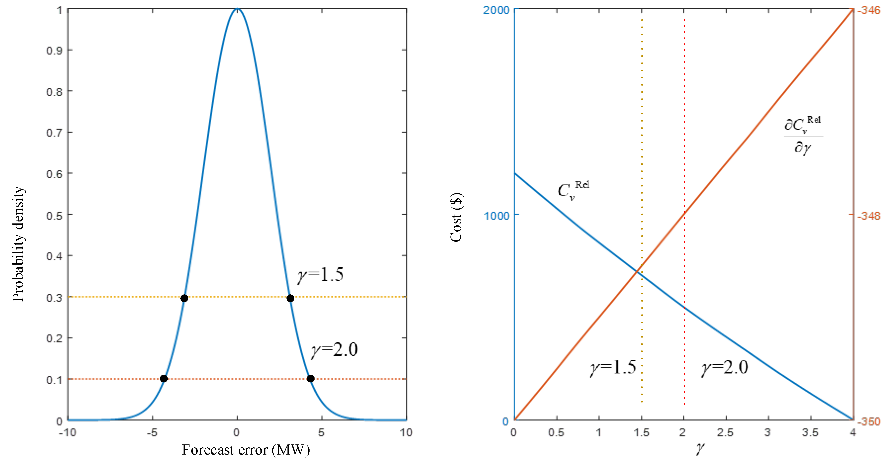
For example, if the parameters of a VRE GenCo is as shown in
Table 1, the relation of reliability and cost is shown in
Figure 3.
Note that parameters can be set to fit the practical situation. If a VRE GenCo does not control its forecast error, then and no reliability cost will occur. If a VRE GenCo increases cost in reliability control, for example in storage, then both fixed cost and variable cost will occur in reliability control. The variable cost is connected to the error range. Note that the first-order-derivative can be quite large when approaches 0, then the form of exponential function may be a better fit. However, in this paper, the variable reliability cost is assumed to be quadratic along with the production cost of thermal units.
If the operation of the market result in an amount of is cleared for (a VRE GenCo) to deliver, bears 2 types of risks: ① Its realized maximum power is lower than . This means negative deviation of power output happened, and has to bear deviation cost. ② Its realized maximum power is higher than . This means has to bear energy curtailment of .
3.2. Day-Ahead forward Market Considering Reserve Services for Variability
Inspired by the authors of [
63], the day-ahead market is cleared by multi-period DC-OPF model for each hour in a day. VREs are allowed to participate in the market. This paper applies DC-OPF model because it is a simplified model while maintains accuracy when certain assumptions are satisfied. The simplicity helps unveiling the patterns of VRE market participation.
There are some basic settings and assumptions as follows.
Assumption 1. The resistance for each branch is negligible compared to the reactance and can therefore be set to 0 [63]. Assumption 2. The voltage magnitude at each node is equal to the base voltage [63]. Assumption 3. The voltage angle difference across any branch is sufficiently small in magnitude [63]. Assumption 4. Thermal GenCos and VRE GenCos can lock income in day-ahead market. The production function of thermal GenCos and reliability function of VRE GenCos have quadratic form, and their first-order derivatives have affine form.
Assumption 5. The ISO will announce the reserve demand for imbalance for the intraday operation before the day-ahead market bidding.
Assumption 6. No-load, start up and shut down cost of units are neglected. Thus, all units can be treated as committed and Security Constrained Unit Commitment (SCUC) problem solving would not be needed.
Assumption 7. The ISO will solve a DC-OPF Security Constrained Economic Distribution (SCED) problem to for each hour of the next 24 h at the beginning of each day in the day-ahead clearing.
Assumption 8. All GenCos are committed.
Assumptions 1–3 are to simplify the computation requirement. Assumptions 4–8 set a basic VRE-participated model of a day-ahead power market. The simplification will not ease the significance of the results and conclusions.
The day-ahead SCED problem (SCED DA) is as follows.
r.t.s.t.We have: , , , , , .
is the production function, for , for . is the production function for ancillary service, which is the reserve service in this problem. also has quadratic form . And the ancillary service can only be provided by thermal GenCos in this setting. is a penalty function to make sure Assumption 3 is satisfied.
Condition (5) considers the node active power balance. is the sum of demand bid by load-serving entities (LSE). is the sum of demand offered by GenCos including thermal and VRE GenCos. is the sum of power drawn from node k by the system. is the Lagrange multiplier of this condition.
Condition (6) considers the Ancillary service requirement. Based on Assumption 6, this paper only deals with short-term reserves. is a hourly reserve requirement proposed by the ISO, and considered as a control factor. It must not be smaller than the sum of reserve quantity offered by the thermal GenCos. It is related to the system balance, and to short-term reserve cost for VRE integration. Note that in a complex practical market, the ancillary service requirement is much more than a short-term requirement. It includes load following, regulation, long-term reserve, reactive compensation, frequency adjustment and so on.
Condition (7) considers the transmission line security constraint. is the maximum magnitude capacity of transmission line km.
Condition (8) claims that the sum of the active power offer and reserve offer cannot exceed the maximum generation capacity. Note that is reported by thermal GenCo.
Condition (9) is the lower output constraint of a VRE GenCo. Note that is reported by thermal GenCos.
Conditions (10) is the output constraint of a VRE GenCo. Note that and are reported by VRE GenCos.
Condition (11) is the value range constraints of variables.
In this model, the marginal generation cost of VRE is treated as 0. However, costs need to be paid if a VRE GenCo wants to maintain a certain level of generation reliability, as described in
Section 3.1. But this cost is not considered by the ISO as part of the objective function. This is a reasonable consideration, because under current spot market mechanism, the production cost is quantity-based.
The day-ahead cleared ancillary service price is .
3.3. Real Time Balance
To simplify the model and make the mechanism trackable, we make another assumption here.
Assumption 9. There is no intra-day sudden outage of a VRE generation unit or a thermal unit or a transmission line.
Assumption 9 means that the variability of active power output of VRE GenCos is the only uncertain factor in the model. By eliminating other uncertain factors, this setting helps analyze the influence of integration of VRE to the cost and efficiency.
The ISO will maintain the system balance by solving another real time SCED problem (SCED RT) as follows. For each real-time period:
r.t.s.t.We have: , , .
In real-time (every hour for simplification), the actual maximum output capacity of a VRE GenCo is realized. is the realized value.
is the penalty function for node load imbalance. We have:
Condition (12) is the real time node balance constraint. It is similar to Condition (15) while a slack variable is allowed. . and are recognized as “imbalance factors”, which is a measurement of the negative effect of the variability of VRE on the system. Based on and , the imbalance cost can be measured. Since the only uncertain factor is the output variation of VRE, the imbalance cost brought by VRE integration can be measured by and . is a penalty factor.
Condition (13) is real time transmission line security constraint.
Condition (14) is the real time output constraint of a thermal GenCo. The lower limit is consistent with the day-ahead report. The upper limit is the sum of cleared day-ahead cleared power output and reserve output.
Condition (15) is the real time output constraint of a VRE GenCo. The lower limit is consistent with the day-ahead report. The upper limit is the minimum of realized maximum output and day-ahead cleared power output.
Condition (16) is the value range constraints of variables.
From model SCED RT, we can see that the system is optimally dispatched based on the real time status of the system.
3.4. Ex-Post Settlement
Ex-post settlement is important for determining the cost of deviation. There are many researchers studying the ex-post settlement mechanism [
64,
65]. In this paper, we adopt the idea proposed by Zheng and Litvinov [
66].
Under the assumption of perfect market and perfect information, from an ISO perspective, for each GenCo agent
, in equilibrium, it faces the following profit maximization problem (PMP). For each period:
s.t.. is the day ahead LMP, is the cleared day ahead reserve price.
The first-order KKT condition of this problem can be formulated as:
The complementarity conditions are:
and
are Lagrange coefficients obtained by solving the SCED DA problem. According to the work of Zheng and Litvinov [
66], if the result of the SCED DA problem can be treated as the equilibrium result of the day ahead situation, then the Karush-Kuhn-Tucker (KKT) condition of the PMP problem gives a good constraint for the ex-post settlement problem. In this paper, we ignored the Conditions (22)–(25), because the ex-post settlement condition is a deviation to the SCED DA result; additionally, we consider learning and strategic behavior for GenCos, then the Conditions (22)–(25) could be too strong and lead to problem infeasibility.
As a result, this paper set the ex-post settlement as the following problem (EXP). For each
:
r.t.s.t. and (w belongs to node k). The solution and give the ex-post price.
and are Lagrange function imbalance factors. is a penalty factor.
Conditions (27) and (28) are respectively the Lagrange function of the active power maximization and reserve power maximization problem in PMP.
The settlement price is as follows:
is an ex-post settlement threshold, and . Condition (30) means that if the actual output deviates from the day-ahead cleared amount and the deviation exceeds a threshold, the ex-post price should be applied.
3.5. Learning and Strategic Behavior of GenCos
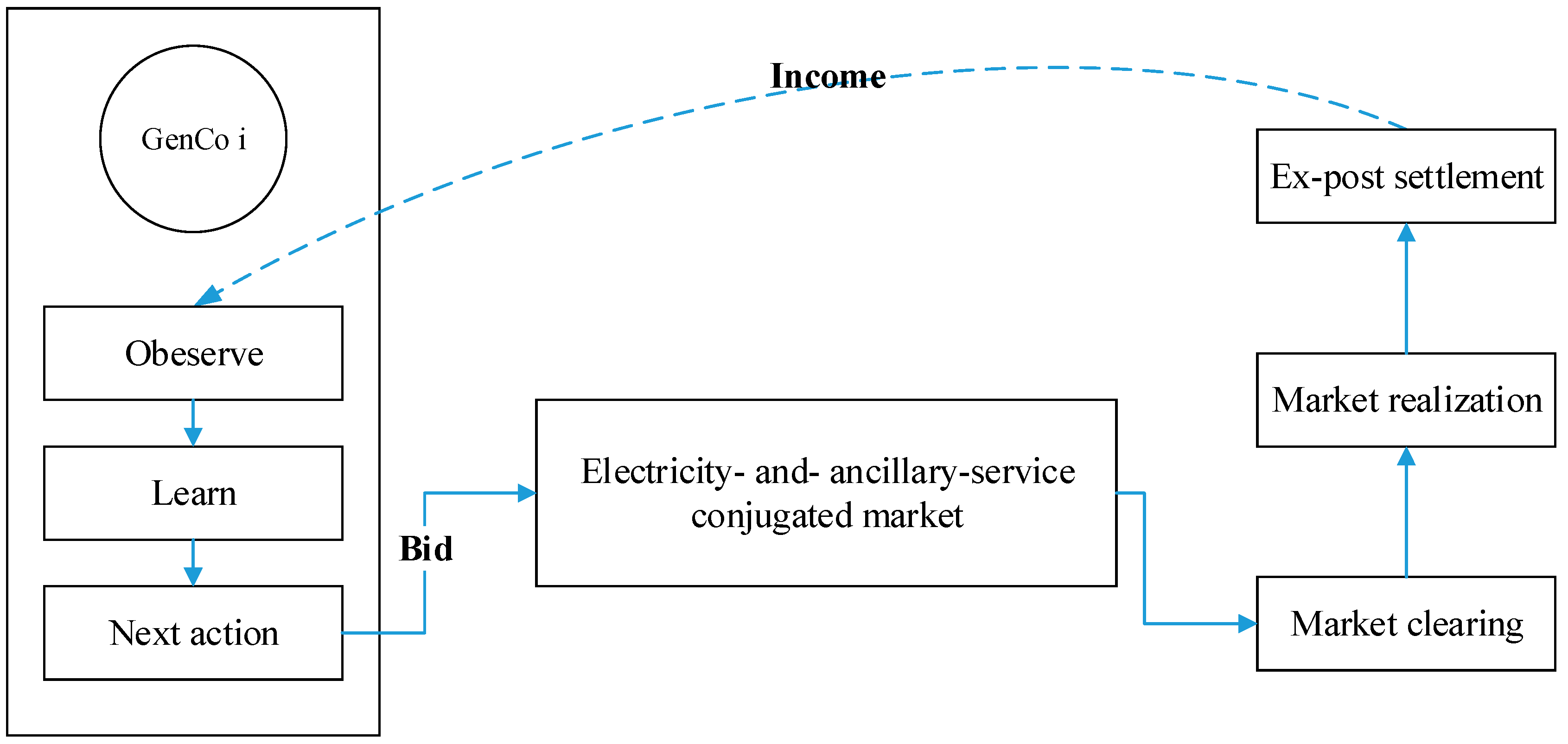
Ideally, GenCos report their true production parameters to the ISO. Under this situation, ISO can clear the market with true marginal condition and reach society optimality. However, there exists information asymmetry in the market. The true production parameters are private information of the GenCos. In the real world, market participators are humans. Human behavior is complicated. In the market, participators will observe the profit brought by their previous action and choose the best action (bid parameters) that brings the most income. This process can be simulated by reinforcement learning method. The process is illustrated in
Figure 4.
This paper considers strategic behaviors of GenCos. For each period, for a VRE GenCo at maximum output level , it can achieve a forecast error level at with mean value at a cost level of . However, can report strategic coefficients (, ) to the ISO, as a result of a learning process. Moreover, can learn to adopt a best value (reliability level) to a day’s operation.
Similarly, a thermal GenCo will learn to strategically report (
,
,
,
) to the ISO in the day ahead market. This paper adopted the famous Erev–Roth reinforcement learning method to simulate the learning behavior of GenCos [
67,
68]. This method imitates the learning process of human being; thus, it grants us a chance to study the influences of learning and strategic behavior. Learning and strategic behavior make the system equilibrium hard to track, but it is a more practical setting than perfect market assumption. The consequences of learning and strategic behavior can be tracked by simulation approach as shown in this paper.
3.6. Case Design and Numerical Simulation
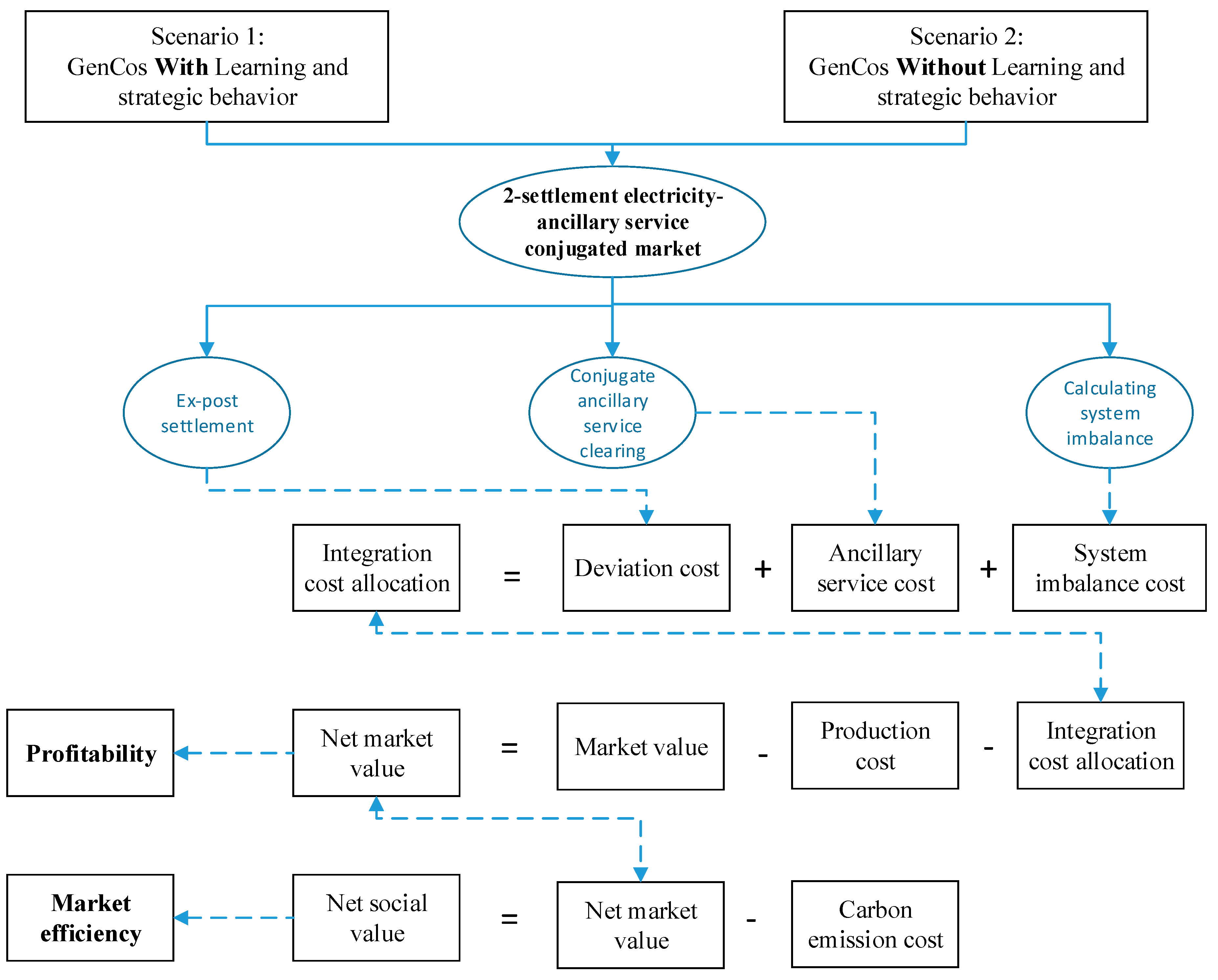
The case design principle is shown in
Figure 5. Two scenarios are set to formulate comparison. Under one scenario, agents do not have learning and strategic behavior while under another scenario agents have learning and strategic behavior. The result comparison can show the influences of the learning and strategic behavior. This paper mainly considers three kinds of trackable integration costs, which are widely considered in practical VRE participated markets. Through the design of the 2-settlement electricity-ancillary service conjugated market in
Section 3.1,
Section 3.2,
Section 3.3,
Section 3.4 and
Section 3.5, they can be simulated numerically. Ex-post settlement will determine deviation cost of VRE, since we rule out other deviations. Conjugate ancillary service clearing will show the cost of ancillary service. Since VRE are the only uncertainty source need for ancillary service, they must bear all the ancillary service cost. System imbalance cost is the cost of lost load. Since the total capacity is enough, load is lost because of the output uncertainty of the VRE.
Profitability of VRE is characterized by their net market value, which is the net income of the VRE in the market. It equals market value minus production cost and minus integration cost. Market efficiency is characterized by the net market value of VRE. It characterized the net benefit the VRE brought to the society.
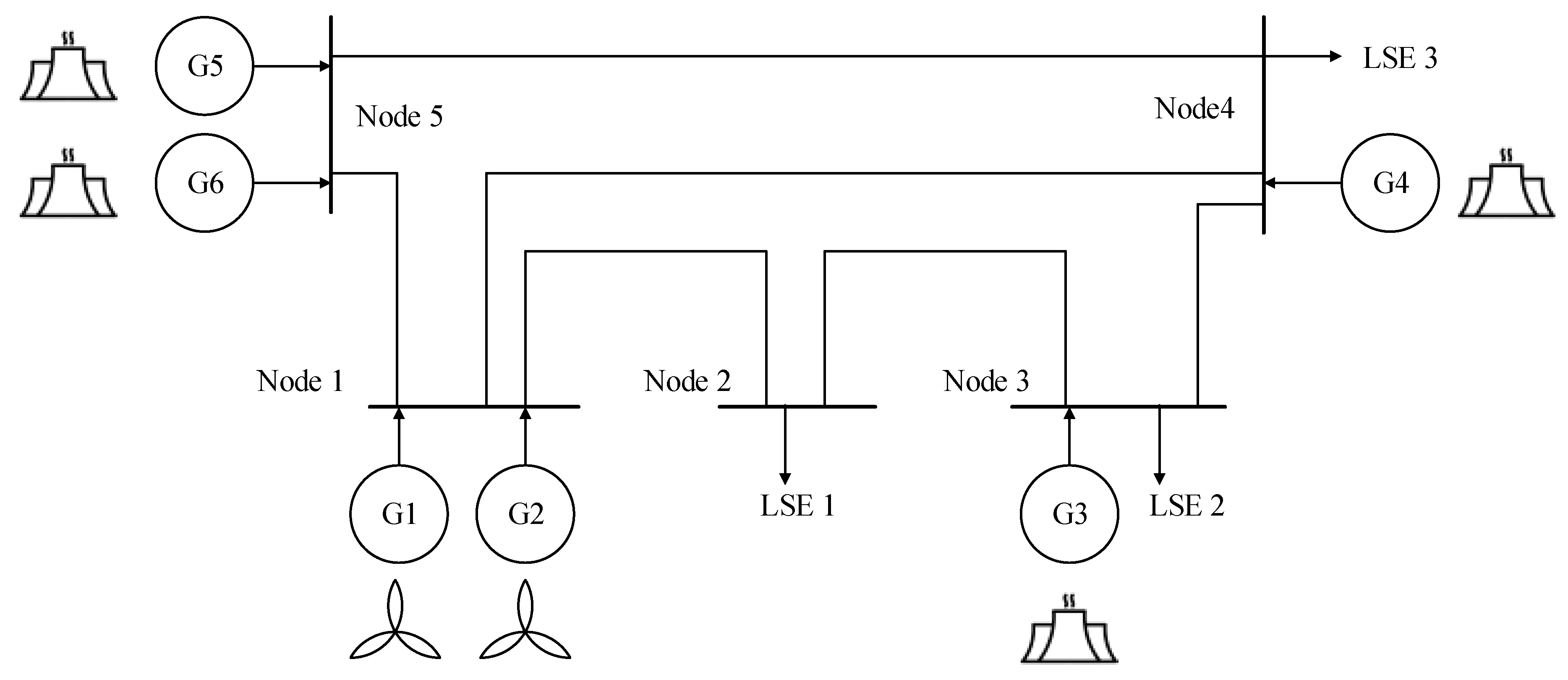
This paper extended the standard 5-node test framework in the work of Sun and Tesfatsion, and Li and Tesfatsion [
63,
69]. The system structure is shown in
Figure 6. There are 6 GenCos and 3 load-serving entities (LSEs). G1 and G2 are VRE GenCos, and the others are thermal GenCos. Initial properties of GenCos are shown in
Table 2. The transmission line properties are shown in
Table 3. All the parameter explanation can be found in the Nomenclatures table at the front of this paper.
The parameter setting is representative. Note that in
Table 2, the reserve cost coefficients are 1/10 of the production coefficients, because reserve cost is usually the no-load cost of the unit. It is significantly smaller than the production cost. For VRE GenCos, GenCo1 and GenCo2 have the same fixed cost, initial money and learning settings. The installed capacity ratio of VRE GenCo is 13.16%. This ratio is representative, because it is nearly the practical ratio of many countries (except for some wind dominant countries such as north European countries).
The simulation process can be found in
Figure 7. At the beginning of the day-ahead market, LSEs provide their load profile to the ISO. To make the result trackable, this paper does not consider price-sensitive bidding and strategic behavior of the LSEs. In other words, all demands are price-inelastic. This paper adopt the 24-h load profile in the work of Sun and Tesfatsion, and Li and Tesfatsion [
63,
69]. To eliminate the influences of load variation between days, the load profile is the same for each day.
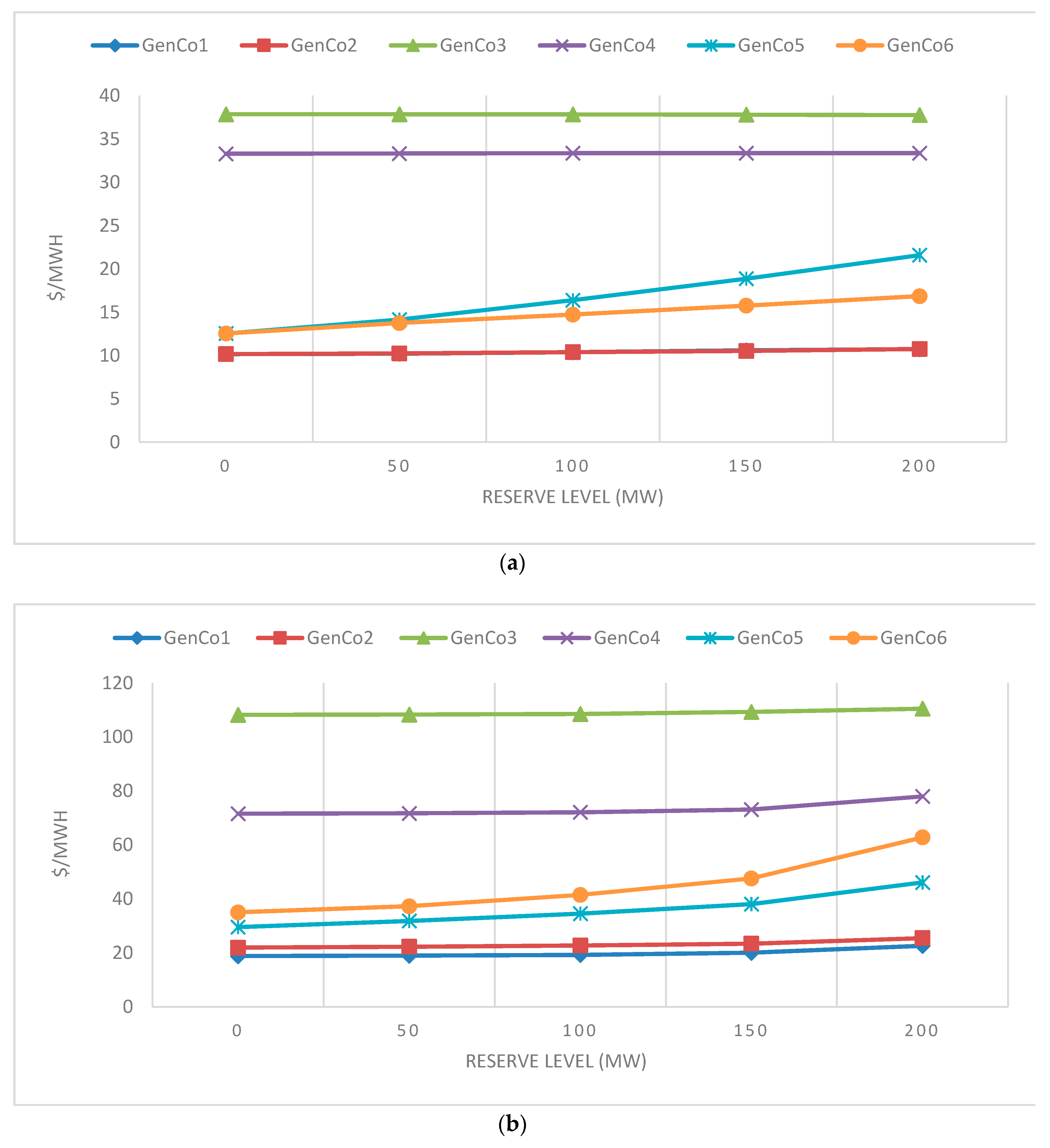
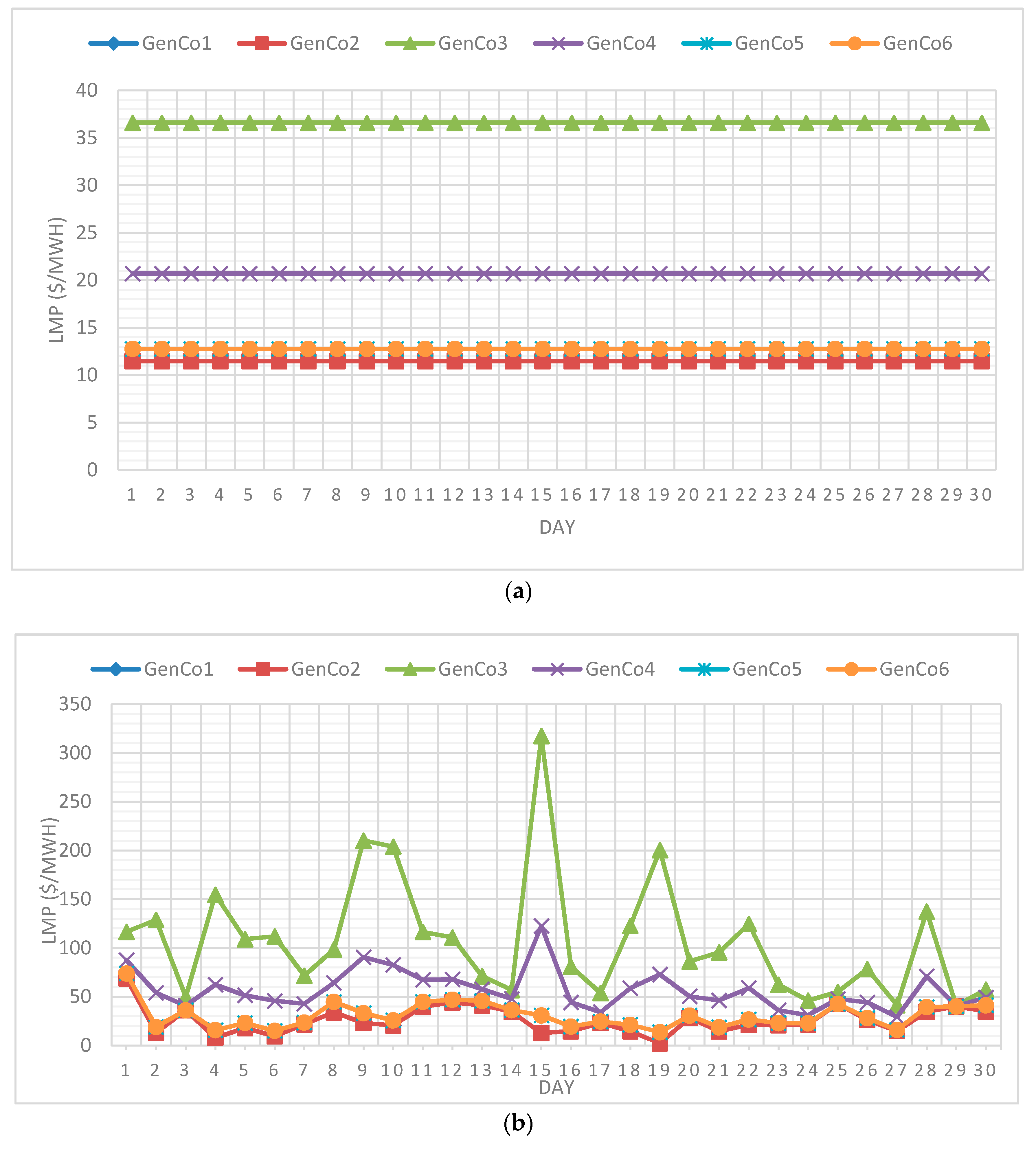
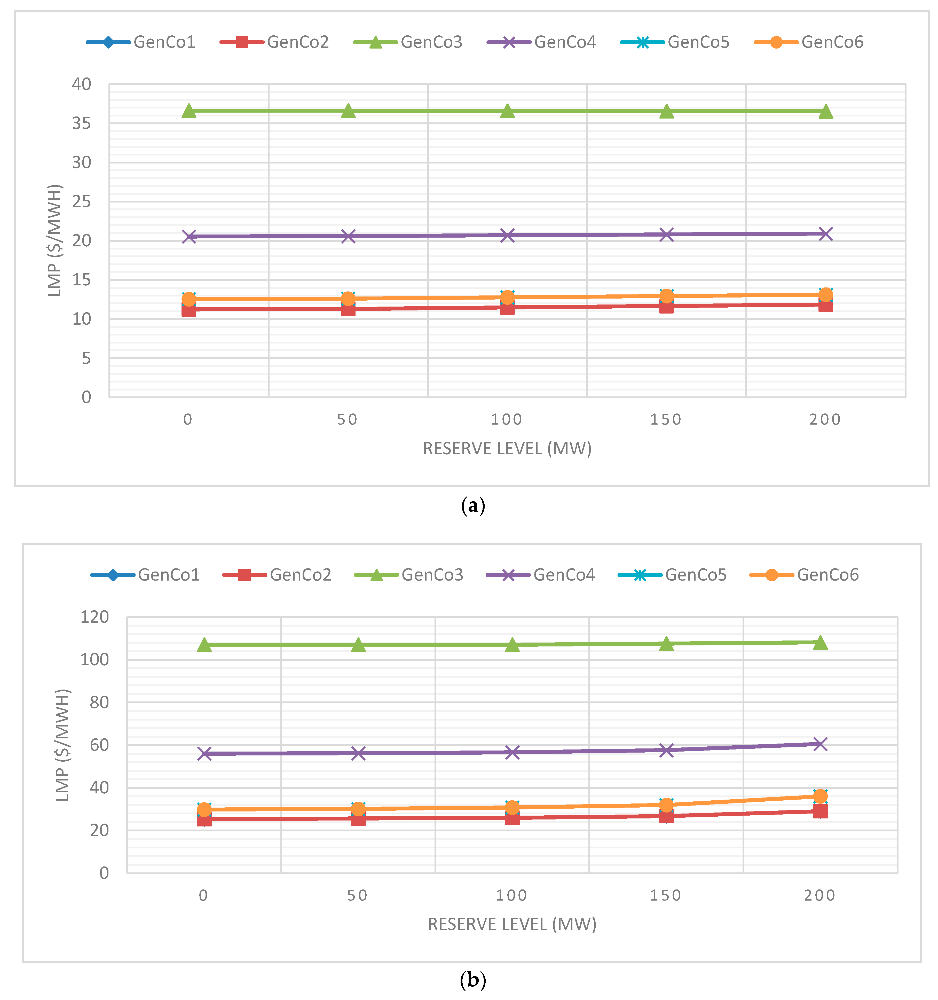
This research carried out two scenarios of test cases, all of which lasted for 30 simulation days. The condition variation is shown in
Table 4. Note that when reserve level is 0 MW, there are no ancillary services for VRE. This will expose the negative influences of the variability of the VRE GenCos. When the reserve level is 200 MW, it covers all of the VRE capacity. Note that when GenCos do not have learning ability, they bid by their true parameter value, and thus the system operation result can be treated as an equilibrium result.


