Robust Sensor Fault Reconstruction via a Bank of Second-Order Sliding Mode Observers for Aircraft Engines

Abstract

This paper deals with sensor faults of aircraft engines under uncertainties using a bank of second-order sliding mode observers (SMOs). In view of the effect of inevitable uncertainties on the fault reconstruction, a method combining $H_{\infty }$ concepts and linear matrix inequalities (LMIs) is proposed, in which a scaling matrix is designed to minimize the gain of the transfer function matrix from uncertainty to reconstruction. However, robust design generally requires that engine outputs outnumber faults. In the case where the above-mentioned requirement is not satisfied, a bank of sliding mode observers is proposed to ensure the degrees of freedom available in robust design. In specific, each observer corresponds to a certain sensor with the hypothesis that the corresponding sensor will not have faults, to create one degree of design freedom for each observer. After fault occurrence, a large estimation error is expected in the observers with wrong hypothesis, and then a logic module is designed to detect sensor faults and obtain the optimal robust sensor fault reconstruction at the same time. The proposed approach is applied to a nonlinear engine component-level-model (CLM) simulation platform, and a numerical study is performed to validate the effectiveness.

1. Introduction

With the increasing demand for higher reliability and safety of aircraft engine, the fault detection and isolation (FDI) system has been widely developed in recent decades [1,2,3]. With sensor being an important part in the control loop, faults occurring in sensors would directly affect, even devastate the quality of the control system, hence more and more importance has been attached to the study of sensor fault diagnosis. Different approaches including model-based methods [4,5] and data-based methods [6] can be found in the literature. Due to the limitation of on-board storage capability of engines, the model-based approach [7], which relies on mathematical model and residual generation [8], has gained more attention from researchers. The main drawback of these approaches lies in their dependence on the accurate dynamic model, which is hard to balance simplicity against accuracy from many actual systems, and the presence of uncertainty will inevitably cause deviations from true states and optimal fault reconstructions [9,10]. Nevertheless, most frameworks of FDI are designed for the linear system in the past decades [11,12]. Model-based fault diagnosis against external disturbance and modeling uncertainties is the most difficult and important issue, especially in the incipient fault detection (IFD) step [13,14,15].

As a model-based method, the sliding mode observer is widely studied in fault diagnosis because of its inherent robustness against uncertainties which satisfies characteristic conditions [16,17,18]. It is able to resist uncertainties by applying proper gain without resorting to any numerical optimization, and then deal with sensor fault [19], actuator fault [20,21], performance change estimation [22], and so on. In sliding mode observers, a non-linear discontinuous term containing the information of output estimation error is designed to make the system converge to the sliding surface [17]. Although the discontinuous switching term makes the chattering phenomenon of fault reconstruction inevitable, proper observer design such as high-order sliding mode can weaken this issue according to the recent research [23]. Higher order sliding modes (HOSM), which eliminate the chattering phenomenon [24,25], are proved to have better performance than first orders. In this paper, a second-order sliding mode observer (SOSMO) is proposed based on the super twisting algorithm (STA) [26] due to its fast convergence rate and robustness against bounded uncertainties. Compared with the standard first order sliding mode observer [17], SOSMOs do have better performance such as small chattering effect [22]. Its stability and finite time convergence under uncertainties is proved through the Lyapunov function [27]. To ascertain the robustness against a class of perturbations wider than that in [27], a family of strict Lyapunov functions is constructed for the STA [28] by JA Moreno and M Osorio. However, the design described above only ensures the finite-time convergence, and the effect of uncertainty on fault reconstruction is still inevitable. In order to minimize this effect, two types of sliding mode observer designs are proposed. The first one is to estimate the uncertainty directly and compensate for the effect of uncertainty into the reconstruction, but this method has strict conditions for application [29]. The second one is to minimize the gain of the transfer matrix from uncertainty to reconstructions through the LMI design, so as to reduce the effect of uncertainty on the reconstruction [17,30,31]. In this paper, the latter approach is adopted for its general applicability in handling more forms of uncertainties and conditions, and the method based on $H_{\infty }$ is widely used for robust fault estimation [22,23,24,25,26,27,28,29,30,31,32,33].

Nevertheless, classical robust design against uncertainties using LMI [33] requires the degrees of freedom available. For sensor fault diagnosis, it means that at least one sensor is ensured to be no fault during operations. In some practical situations, certain sensors are actually less vulnerable than others, and the above-mentioned assumption is not unrealistic [17]. However, for aircraft engines, all sensors work in the environment of high temperature, high pressure, and high rotation speed, thus, all risk damages. In this situation, there is not enough design freedom left for robust design against any uncertainty. Therefore, a framework constituting a bank of sliding mode observers is proposed in this paper. The architecture contains 7 sliding mode observers where 7 is the number of considered sensors. Each observer corresponds to a certain sensor, with the specific hypothesis that the corresponding sensor is guaranteed not to malfunction, for example, the first observer is constructed on the premise that the first sensor is reliable. This design ascertains that each observer can have a degree of design freedom. In the event that a fault occurs, reconstructions except the SMOs using the correct assumptions will produce large reconstruction errors. A scalar indicator is designed to evaluate the residual of each observer and the fault diagnosis module is established to detect and reconstruct the sensor faults.

This paper is organized as follows: The system description of aircraft engines is shown in Section 2, and the rest part of this section is concerned about the design of the bank of SMOs, containing the robust design based on STA using LMI and the whole framework of the FDI system. The proposed method is applied to the engine system which is depicted in Section 3. The whole FDI system’s validation is proved in simulation and experiment. And conclusions are given in Section 4.

2. Design of the Bank of Robust Sliding Mode Observers

A twin-spool commercial turbofan engine is used in this paper. The structure of the engine is shown in Figure 1. The air is compressed by a low pressure compressor (LPC) and a high pressure compressor (HPC), mixed with fuel, and injected into the combustor for combustion. A high pressure turbine (HPT) and a low pressure turbine (LPT) are driven by gases of high pressure and temperature generated by combustion, and drive the two compressors through two rotating shafts. The notations in this paper are shown in Table 1.

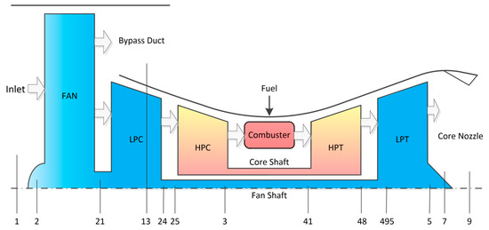
Figure 1. Structure of the engine.

Table 1. The descriptions of the notations.

Notation	Description
H	Flight height
Ma	Mach number
Wf	Fuel flow rate
T25	LPC outlet temperature
P25	LPC outlet pressure
T3	HPC outlet temperature
P3	HPT outlet pressure
T495	Exhaust gas temperature
NL	Low pressure rotor speed
NH	High pressure rotor speed

The engine is inherently nonlinear on account of the thermal effects, complex mechanical structures and so on. A component level model (CLM) is used in this paper which is a nonlinear simulation of the turbofan engine with high fidelity, and it has been validated versus testing data [34]. Based on the CLM, a state variable model (SVM), which is a linear engine dynamic model, can be obtained and represented by the following state-space equations [34]:

$$\dot{\mathit{x}}(t)=\mathit{Ax}(t)+\mathit{Bu}(t),$$

(1)

$$\mathit{y}(t)=\mathit{Cx}(t)+\mathit{Du}(t),$$

(2)

where $\mathit{x}(t)\in {ℝ}^n$, $\mathit{y}(t)\in {ℝ}^p$, $\mathit{u}(t)\in {ℝ}^m$ are the state variables, measurable outputs, and measurable inputs, respectively. $\mathit{A}\in {ℝ}^{n\times n},\mathit{B}\in {ℝ}^{n\times m},\mathit{C}\in {ℝ}^{p\times n}$, and $\mathit{D}\in {ℝ}^{p\times m}$ are real known matrices. $\mathit{x}(t)={\left[\begin{array}{cc}{N}_L& N_H\end{array}\right]}^{\mathrm{T}}$, $\mathit{y}(t)={\left[\begin{array}{ccccccc}{N}_L& N_H& T_{25}& P_{25}& T_3& P_3& EGT\end{array}\right]}^{\mathrm{T}}$, and $u(t)=W_f$, that is, $n=2,p=7$ and $m=1$.

The nominal model does not take into account uncertainties such as parameter uncertainties and external disturbances. Under the influence of simultaneous sensor faults and uncertainty, the real engine dynamic system can be written as:

$$\dot{\mathit{x}}(t)=\mathit{Ax}(t)+\mathit{Bu}(t)+{\mathit{Q}}_1\mathit{\xi }(\mathit{x},t),$$

(3)

$$\mathit{y}(t)=\mathit{Cx}(t)+\mathit{Du}(t)+\mathit{Nf}(t)+{\mathit{Q}}_2\mathit{\xi }(\mathit{x},t),$$

(4)

where the signal $\mathit{f}(t)\in {ℝ}^q$ represents the sensor faults imposed upon the system with $p\ge q$ and $\mathit{N}\in {ℝ}^{p\times q}$ as the distribution matrix. The term $\mathit{\xi }(\mathit{x},t)\in {ℝ}^r$ is considered as any uncertainty present. ${\mathit{Q}}_1\in {ℝ}^{p\times r}$, ${\mathit{Q}}_2\in {ℝ}^{n\times r}$ are real known distribution matrices. Sensor fault signals and uncertainties are unknown but bounded and satisfy the following conditions:

$$\Vert \mathit{f}(t)\Vert \le {\epsilon }_1,\Vert \dot{\mathit{f}}(t)\Vert \le {\epsilon }_2,\Vert \mathit{\xi }(t)\Vert \le \eta ,$$

(5)

where ${\epsilon }_1,{\epsilon }_2$, and $\eta$ are known scalars, and $\Vert ·\Vert$ represents Euclidean norm of the vector. All parameters are normalized and the detailed values are calculated by the data extracted from the engine design point.

Define a new output $\mathit{z}(t)\in {ℝ}^p$ which is a filter version satisfying:

$$\mathit{z}(t)=-{\mathit{A}}_f\mathit{z}(t)+{\mathit{A}}_f\mathit{y}(t),$$

(6)

where ${\mathit{A}}_f$ is a designed stable real matrix. According to Equations (3), (4) and (6), the uncertain system can be rewritten as an augmented state-space system given by:

$$\left[\begin{array}{c}\dot{\mathit{x}}(t)\\ \dot{\mathit{z}}(t)\end{array}\right]=\underset{{\mathit{A}}_a}{\underbrace{\left[\begin{array}{cc}\mathit{A}& \mathit{0}\\ {\mathit{A}}_f\mathit{C}& -{\mathit{A}}_f\end{array}\right]}}\left[\begin{array}{c}\mathit{x}(t)\\ \mathit{z}(t)\end{array}\right]+\underset{{\mathit{B}}_a}{\underbrace{\left[\begin{array}{c}\mathit{B}\\ {\mathit{A}}_f\mathit{D}\end{array}\right]}}u(t)+\underset{{\mathit{M}}_a}{\underbrace{\left[\begin{array}{c}\mathit{0}\\ {\mathit{A}}_f\mathit{N}\end{array}\right]}}\mathit{f}(t)+\underset{{\mathit{Q}}_a}{\underbrace{\left[\begin{array}{c}{\mathit{Q}}_1\\ {\mathit{A}}_f{\mathit{Q}}_2\end{array}\right]}}\mathit{\xi }(\mathit{x},t),$$

(7)

$$\mathit{z}(t)=\underset{{\mathit{C}}_a}{\underbrace{\left[\begin{array}{cc}\mathit{0}& {\mathit{I}}_p\end{array}\right]}}\left[\begin{array}{c}\mathit{x}(t)\\ \mathit{z}(t)\end{array}\right],$$

(8)

Define ${\mathit{x}}_a(t)={[\begin{array}{cc}\mathit{x}{(t)}^{\mathrm{T}}& \mathit{z}{(t)}^{\mathrm{T}}\end{array}]}^{\mathrm{T}}\in {ℝ}^{n+p}$ are augmented state variables. ${\mathit{A}}_a$, ${\mathit{B}}_a$, ${\mathit{C}}_a$, ${\mathit{M}}_a$ and ${\mathit{Q}}_a$ are augmented matrices with appropriate dimensions.

To underpin the rest part of this method, the following conditions must be satisfied:

• The fault distribution matrix ${\mathit{M}}_a$ has full rank of columns and satisfies the equation $rank({\mathit{C}}_a{\mathit{M}}_a)=rank({\mathit{M}}_a)=r$.
• Let the triple $\left({\mathit{A}}_a,{\mathit{M}}_a,{\mathit{C}}_a\right)$ represent the linear system and the invariant zeros (if any) of $\left({\mathit{A}}_a,{\mathit{M}}_a,{\mathit{C}}_a\right)$ are Hurwitz.

Considering the special structure of ${\mathit{M}}_a$, ${\mathit{C}}_a$, and the square matrix ${\mathit{A}}_f$ with full rank, the first condition can be proved by:

$$\begin{array}{cc}\hfill rank\left({\mathit{M}}_a\right)& =rank\left(\left[\begin{array}{c}\mathit{0}\\ {\mathit{A}}_f\mathit{N}\end{array}\right]\right)=rank\left({\mathit{A}}_f\mathit{N}\right)\hfill \\ & =rank\left(\mathit{N}\right)=q\hfill \end{array}$$

(9)

$$\begin{array}{cc}\hfill rank\left({\mathit{C}}_a{\mathit{M}}_a\right)& =rank\left(\left[\begin{array}{cc}\mathit{0}& {\mathit{I}}_p\end{array}\right]\left[\begin{array}{c}\mathit{0}\\ {\mathit{A}}_f\mathit{N}\end{array}\right]\right)\hfill \\ & =rank\left({\mathit{A}}_f\mathit{N}\right)=rank\left(\mathit{N}\right)=q\hfill \end{array}$$

(10)

The zeros of $\left({\mathit{A}}_a,{\mathit{M}}_a,{\mathit{C}}_a\right)$ are given by the values of $s$ which make the Rosenbrock matrix $\mathit{R}$ lose rank [17], where:

$$\mathit{R}=\left[\begin{array}{cc}s\mathit{I}-{\mathit{A}}_a& -{\mathit{M}}_a\\ {\mathit{C}}_a& \mathit{0}\end{array}\right]=\left[\begin{array}{ccc}s{\mathit{I}}_n-\mathit{A}& \mathit{0}& \mathit{0}\\ -{\mathit{A}}_f\mathit{C}& s{\mathit{I}}_p+{\mathit{A}}_f& {\mathit{A}}_f\mathit{N}\\ \mathit{0}& {\mathit{I}}_p& \mathit{0}\end{array}\right].$$

(11)

In consideration of the fact that the matrix ${\mathit{A}}_f$ is square with full rank, the Rosenbrock matrix loses rank if $rank\left(s{\mathit{I}}_n-\mathit{A}\right)<n$. The invariant zeros of $\left({\mathit{A}}_a,{\mathit{M}}_a,{\mathit{C}}_a\right)$ are contained in the eigenvalues of $\mathit{A}$ and so if the open-loop system is stable, system is detectable and minimum phase [17].

Based on the uncertain system in Equations (7) and (8), a sliding mode observer can be designed in the following form:

$${\dot{\widehat{\mathit{x}}}}_a(t)={\mathit{A}}_a{\widehat{\mathit{x}}}_a(t)+{\mathit{B}}_{a}u(t)+{\mathit{G}}_n\mathit{v}-{\mathit{G}}_l{\mathit{e}}_z(t),$$

(12)

$$\widehat{\mathit{z}}(t)={\mathit{C}}_a{\widehat{\mathit{x}}}_a(t),$$

(13)

where $\left({\widehat{\mathit{x}}}_a(t),\widehat{\mathit{z}}(t)\right)$ are the estimates of $\left({\mathit{x}}_a(t),\mathit{z}(t)\right)$ and $\mathit{v}(t)\in {ℝ}^p$ is a nonlinear discontinuous term. Define $\mathit{e}(t):={\widehat{\mathit{x}}}_a(t)-{\mathit{x}}_a(t)$ and ${\mathit{e}}_z(t)=\widehat{\mathit{z}}(t)-\mathit{z}(t)$ as the state estimation and output estimation errors, respectively. The output error feedback term ${\mathit{G}}_l{\mathit{e}}_z(t)$ is attached to the observer to enlarge the size of the sliding patch. Both ${\mathit{G}}_l\in {ℝ}^{(n+p)\times p}$ and ${\mathit{G}}_n\in {ℝ}^{(n+p)\times p}$ are design matrices to be determined. Assuming that the gain ${\mathit{G}}_l$ and ${\mathit{G}}_n$ have the structure:

$${\mathit{G}}_n=\left[\begin{array}{c}\mathit{0}\\ {\mathit{I}}_p\end{array}\right],{\mathit{G}}_l=\left[\begin{array}{c}\mathit{0}\\ -{\mathit{A}}_f\end{array}\right].$$

(14)

Then based on the super-twisting algorithm (STA), the term $\mathit{v}(t)$ is designed component-wise as [28]:

$$v_i(t)=-k_{1}sign(e_{z,i}(t))|e_{z,i}(t){|}^{\frac{1}{2}}+d_i(t),$$

(15)

$${\dot{d}}_i(t)=-k_{2}sign(e_{z,i}(t))i=1,2,\cdots ,p,$$

(16)

where $k_1$ and $k_2$ are design scalars to be determined. $\mathit{d}(t)$ is an intermediate variable. The subscript $i$ represents $i$th element of variables.

According to the definitions of $\mathit{e}(t)$ and ${\mathit{e}}_z(t)$, the error system can be obtained from Equations (7), (8), (12) and (13):

$$\dot{\mathit{e}}(t)={\mathit{A}}_a\mathit{e}(t)-{\mathit{G}}_l{\mathit{e}}_z(t)+{\mathit{G}}_n\mathit{v}(t)-{\mathit{M}}_a\mathit{f}(t)-{\mathit{Q}}_a\mathit{\xi }(\mathit{x},t),$$

(17)

$${\mathit{e}}_z(t)={\mathit{C}}_a\mathit{e}(t).$$

(18)

Due to the special structure of ${\mathit{C}}_a$ in Equation (8), the state estimation error can be partitioned as $\mathit{e}(t)={[\begin{array}{cc}{\mathit{e}}_1{(t)}^{\mathrm{T}}& {\mathit{e}}_z{(t)}^{\mathrm{T}}\end{array}]}^{\mathrm{T}}$ where ${\mathit{e}}_1(t)\in {ℝ}^n$. Then the error system can be rewritten as:

$$\left[\begin{array}{c}{\dot{\mathit{e}}}_1(t)\\ {\dot{\mathit{e}}}_z(t)\end{array}\right]=\left[\begin{array}{cc}\mathit{A}& \mathit{0}\\ {\mathit{A}}_f\mathit{C}& -{\mathit{A}}_f\end{array}\right]\left[\begin{array}{c}{\mathit{e}}_1(t)\\ {\mathit{e}}_z(t)\end{array}\right]+\left[\begin{array}{c}\mathit{0}\\ {\mathit{I}}_p\end{array}\right]\mathit{v}(t)-\left[\begin{array}{c}\mathit{0}\\ -{\mathit{A}}_f\end{array}\right]{\mathit{e}}_z(t)-\left[\begin{array}{c}\mathit{0}\\ {\mathit{A}}_f\mathit{N}\end{array}\right]\mathit{f}(t)-\left[\begin{array}{c}{\mathit{Q}}_1\\ {\mathit{A}}_f{\mathit{Q}}_2\end{array}\right]\mathit{\xi }(\mathit{x},t).$$

(19)

The above equation can be further written in the following form:

$${\dot{\mathit{e}}}_1(t)=\mathit{A}{\mathit{e}}_1(t)-{\mathit{Q}}_1\mathit{\xi }(t),$$

(20)

$${\dot{\mathit{e}}}_z(t)={\mathit{A}}_f\mathit{C}{\mathit{e}}_1(t)+\mathit{\nu }(t)-{\mathit{A}}_f\mathit{Nf}(t)-{\mathit{A}}_f{\mathit{Q}}_2\mathit{\xi }(\mathit{x},t),$$

(21)

and from the definition of $\mathit{v}(t)$, the output error system in Equation (21) becomes (component-wise):

$$\{\begin{array}{cc}\hfill {\dot{e}}_{z,i}(t)& ={({\mathit{A}}_f\mathit{C})}_i{\mathit{e}}_1(t)+[-k_{1}sign(e_{z,i}(t))|e_{z,i}(t){|}^{\frac{1}{2}}+d_i(t)]-{({\mathit{A}}_f\mathit{N})}_i\mathit{f}(t)-{({\mathit{A}}_f{\mathit{Q}}_2)}_i\mathit{\xi }(\mathit{x},t)\hfill \\ & =[-k_{1}sign(e_{z,i}(t))|e_{z,i}(t){|}^{\frac{1}{2}}]+[{({\mathit{A}}_f\mathit{C})}_i{\mathit{e}}_1(t)-{({\mathit{A}}_f\mathit{N})}_i\mathit{f}(t)-{({\mathit{A}}_f{\mathit{Q}}_2)}_i\mathit{\xi }(\mathit{x},t)+d_i(t)]\hfill \\ \hfill {\dot{d}}_i(t)& =-k_{2}sign(e_{z,i}(t))i=1,2,\cdots ,p\hfill \end{array},$$

(22)

where ${({\mathit{A}}_f\mathit{C})}_i$, ${({\mathit{A}}_f\mathit{N})}_i$, and ${({\mathit{A}}_f{\mathit{Q}}_2)}_i$ represent the $i$th row of the corresponding matrices, respectively. For simplicity, define nominal variables:

$${\mathit{d}}_t(t):={\mathit{A}}_f\mathit{C}{\mathit{e}}_1(t)-{\mathit{A}}_f\mathit{Nf}(t)+\mathit{d}(t),$$

(23)

$$\varphi (t):={\mathit{A}}_f\mathit{C}{\dot{\mathit{e}}}_1(t)-{\mathit{A}}_f\mathit{N}\dot{\mathit{f}}(t),$$

(24)

and the error system can be rewritten as:

$$\{\begin{array}{l}{\dot{e}}_{z,i}(t)=[-k_{1}sign(e_{z,i}(t))|e_{z,i}(t){|}^{\frac{1}{2}}]+d_{t,i}(t)-{({\mathit{A}}_f{\mathit{Q}}_2)}_i\mathit{\xi }(\mathit{x},t)\\ {\dot{d}}_{t,i}(t)=-k_{2}sign(e_{z,i}(t))+\varphi (t)i=1,2,\cdots ,p\end{array},$$

(25)

the term $\mathit{v}(t)$ has been designed to switch discontinuously around the sliding surface $\mathit{S}=\left\{\mathit{e}(t):{\mathit{C}}_a\mathit{e}(t)=\mathit{0}\right\}$ and to drive the trajectories of $\mathit{e}(t)$ to $\mathit{S}$. From inequality (5) and the definition of $\varphi (t)$, the existence of a constant $L$ is ensured, such that the inequality:

$$\Vert \varphi (t)\Vert \le L,$$

(26)

holds for any possible $t$.

The output error system in Equation (25) is a standard super-twisting structure with disturbance term. Then the design process of the two important coefficients $k_1$ and $k_2$ in Equations (15) and (16) is as follows [28]:

• Choose positive constants $\left(\beta ,\gamma \right)$ satisfying $0\text{<}\beta <1$, $\gamma >1$, and $\beta \ast \gamma >1$.
• Calculate positive constants $(\mu ,\alpha )$ where:

  $$\mu =\frac{(\beta -2\frac{1}{\gamma })\beta +1}{1-{\beta }^2},\alpha =\frac{\beta -\frac{1}{\gamma }}{1-{\beta }^2}.$$

  (27)
• Given such values of $\left(\beta ,\gamma \right)$ and $(\mu ,\alpha )$, the gains can be calculated as:

  $$k_1=\mu \sqrt{\frac{2\gamma }{(1-\beta )\alpha }}\sqrt{L},k_2=\frac{\beta +1}{1-\beta }L.$$

  (28)

The gains $k_1,k_2$ based on the recipe in [28] assure the robust, finite time stability of the super-twisting structure with disturbance term, and ensures that a sliding motion can be achieved (${\mathit{e}}_z(t)={\dot{\mathit{e}}}_z(t)=\mathit{0}$). The proof of standard super-twisting structure stability can consult the Lyapunov stability theorem in literature [28]. Once the system state is reached and maintained on the sliding surface $\mathit{S}$, the error system defined by Equations (20) and (21) can be written as:

$${\dot{\mathit{e}}}_1(t)=\mathit{A}{\mathit{e}}_1(t)-{\mathit{Q}}_1\mathit{\xi }(t),$$

(29)

$$\mathit{0}={\mathit{A}}_f\mathit{C}{\mathit{e}}_1(t)+{\mathit{\nu }}_{eq}(t)-{\mathit{A}}_f\mathit{Nf}(t)-{\mathit{A}}_f{\mathit{Q}}_2\mathit{\xi }(\mathit{x},t),$$

(30)

where ${\mathit{v}}_{eq}(t)$ is the so-called equivalent output error injection. This is not the term $\mathit{v}(t)$ which is applied to the system, but rather, the averaged injection used to maintain the sliding motion (${\mathit{e}}_z(t)={\dot{\mathit{e}}}_z(t)=\mathit{0}$), and it can be obtained by filtering.

In the case where the uncertainties are not taken into account, i.e., $\mathit{\xi }(\mathit{x},t)=\mathit{0}$, the existence of the fact ${\mathit{e}}_1(t)\to \mathit{0}$ in finite time is ensured. Hence the reconstruction of $\mathit{f}(t)$ from the equivalent injection signal will be in the following form:

$$\widehat{\mathit{f}}(t)={({\mathit{A}}_f\mathit{N})}^{-1}{\mathit{v}}_{eq}(t),$$

(31)

where $\widehat{\mathit{f}}(t)$ is the estimation of the real sensor faults without robust design.

However, the actual system is always affected by uncertainties. In the case where $\mathit{\xi }(\mathit{x},t)\ne \mathit{0}$, the above attempted reconstruction $\widehat{\mathit{f}}(t)$ will be corrupted by the exogenous factor $\mathit{\xi }(\mathit{x},t)$. To minimize the influence of the uncertainty on the reconstruction, a scaling of the equivalent output injection signal $v_{eq}(t)$ is demanded to be chosen. To this end define:

$${\mathit{W}}_{sc}=\left[\begin{array}{cc}{\mathit{W}}_1& {\mathit{M}}_0{}^{-1}\end{array}\right],$$

(32)

where ${\mathit{W}}_1\in {ℝ}^{p\times (p-q)}$ is the design freedom to be determined and ${\mathit{M}}_0\in {ℝ}^{r\times r}$ is a nonsingular design matrix.

If condition 1 is satisfied it can be proven that there exists an orthogonal matrix $\mathit{T}\in {ℝ}^{p\times p}$, where:

$${\mathit{T}}^{\mathrm{T}}\left({\mathit{A}}_f\mathit{N}\right)=\left[\begin{array}{c}\mathit{0}\\ {\mathit{M}}_0\end{array}\right]\begin{array}{c}\updownarrow \\ \updownarrow \end{array}\begin{array}{c}p-q\\ q\end{array},$$

(33)

the solution of $\mathit{T}$ can be obtained by ‘QR’ decomposition of $\left({\mathit{A}}_f\mathit{N}\right)$.

Define a would-be reconstruction signal as:

$${\widehat{\mathit{f}}}_r(t)={\mathit{W}}_{sc}{\mathit{T}}^{\mathrm{T}}{\mathit{v}}_{eq}(t).$$

(34)

Re-arranging (29) and (30) as:

$${\dot{\mathit{e}}}_1(t)=\mathit{A}{\mathit{e}}_1(t)-{\mathit{Q}}_1\mathit{\xi }(\mathit{x},t),$$

(35)

$${\mathit{\nu }}_{eq}=-{\mathit{A}}_f\mathit{C}{\mathit{e}}_1(t)+{\mathit{A}}_f\mathit{Nf}(t)+{\mathit{A}}_f{\mathit{Q}}_2\mathit{\xi }(\mathit{x},t).$$

(36)

Pre-multiplying (36) by ${\mathit{W}}_{sc}{\mathit{T}}^{\mathrm{T}}$ obtains:

$${\widehat{\mathit{f}}}_r(t)=-{\mathit{W}}_{sc}{\mathit{T}}^{\mathrm{T}}{\mathit{A}}_f\mathit{C}{\mathit{e}}_1(t)+{\mathit{W}}_{sc}{\mathit{T}}^{\mathrm{T}}{\mathit{A}}_f\mathit{Nf}(t)+{\mathit{W}}_{sc}{\mathit{T}}^{\mathrm{T}}{\mathit{A}}_f{\mathit{Q}}_2\mathit{\xi }(\mathit{x},t).$$

(37)

Remark 1.

Notice that ${\mathit{W}}_{sc}{\mathit{T}}^{\mathrm{T}}{\mathit{A}}_f\mathit{N}=\left[\begin{array}{cc}{\mathit{W}}_1& {\mathit{M}}_0{}^{-1}\end{array}\right]{\left[\begin{array}{cc}\mathit{0}& {\mathit{M}}_0{}^{\mathrm{T}}\end{array}\right]}^{\mathrm{T}}={\mathit{I}}_q$, the special structure of the scaling matrix ${\mathit{W}}_{sc}$ in Equation (32) is aim to decouple sensor faults and exogenous signal and leave a certain degree of design freedom to minimize the effect of the exogenous signal on the reconstruction.

Theorem 1.

Considering the system from (35) and (37), it can be rewritten as:

$${\dot{\mathit{e}}}_1(t)={\mathit{A}}^{\prime }{\mathit{e}}_1(t)+{\mathit{B}}^{\prime }\mathit{\xi }(\mathit{x},t),$$

(38)

$${\widehat{\mathit{f}}}_r(t)={\mathit{C}}^{\prime }{\mathit{e}}_1(t)+{\mathit{D}}^{\prime }\mathit{\xi }(\mathit{x},t)+\mathit{f}(t),$$

(39)

where ${\mathit{A}}^{\prime }=\mathit{A}$, ${\mathit{B}}^{\prime }=-{\mathit{Q}}_1$, ${\mathit{C}}^{\prime }=-{\mathit{W}}_{sc}{\mathit{T}}^{\mathrm{T}}{\mathit{A}}_f\mathit{C}$, and ${\mathit{D}}^{\prime }={\mathit{W}}_{sc}{\mathit{T}}^{\mathrm{T}}{\mathit{A}}_f{\mathit{Q}}_2$. The following statements are equivalent.

1.

The system is asymptotically stable and the gain of transfer matrix$\mathit{G}(s)$does not exceed$\kappa \in {ℝ}^{+}$(${\Vert G(s)\Vert }_{\infty }<\kappa$) where:

$$\mathit{G}(s)\triangleq {\mathit{C}}^{\prime }{(s\mathit{I}-{\mathit{A}}^{\prime })}^{-1}{\mathit{B}}^{\prime }+{\mathit{D}}^{\prime }.$$

(40)

2.

There exists a symmetric matrix$P>0$satisfying:

$$\left[\begin{array}{ccc}{\mathit{PA}}^{\prime }+{{\mathit{A}}^{\prime }}^{\mathrm{T}}\mathit{P}& {\mathit{PB}}^{\prime }& {{\mathit{C}}^{\prime }}^{\mathrm{T}}\\ {{\mathit{B}}^{\prime }}^{\mathrm{T}}\mathit{P}& -\kappa \mathit{I}& {{\mathit{D}}^{\prime }}^{\mathrm{T}}\\ {\mathit{C}}^{\prime }& {\mathit{D}}^{\prime }& -\kappa \mathit{I}\end{array}\right]\prec 0.$$

(41)

Proof of Theorem 1.

See Appendix A.

                                 □

Therefore:

$${\widehat{\mathit{f}}}_r(t)=\mathit{f}(t)+\mathit{G}(s)\mathit{\xi }(\mathit{x},t),$$

(42)

where the transfer matrix $\mathit{G}(s)={\mathit{W}}_{sc}{\mathit{T}}^{\mathrm{T}}{\mathit{A}}_f\mathit{C}{(s\mathit{I}-\mathit{A})}^{-1}{\mathit{Q}}_1+{\mathit{W}}_{sc}{\mathit{T}}^{\mathrm{T}}{\mathit{A}}_f{\mathit{Q}}_2$ derived from (38) and (39).

The effect from $\mathit{\xi }(\mathit{x},t)$ to ${\widehat{\mathit{f}}}_r(t)$ can be minimized by choosing the appropriate ${\mathit{W}}_1$. Based on Theorem 1, the $L_2$ gain of $\mathit{G}(s)$ will not exceed $\kappa$ if the following inequality can be satisfied:

$$\left[\begin{array}{ccc}\mathit{PA}+{\mathit{A}}^{\mathrm{T}}\mathit{P}& -\mathit{P}{\mathit{Q}}_1& -{({\mathit{W}}_{sc}{\mathit{T}}^{\mathrm{T}}{\mathit{A}}_f\mathit{C})}^{\mathrm{T}}\\ -{\mathit{Q}}_1{}^{\mathrm{T}}\mathit{P}& -\kappa {\mathit{I}}_r& {({\mathit{W}}_{sc}{\mathit{T}}^T{\mathit{A}}_f{\mathit{Q}}_2)}^{\mathrm{T}}\\ -{\mathit{W}}_{sc}{\mathit{T}}^{\mathrm{T}}{\mathit{A}}_f\mathit{C}& {\mathit{W}}_{sc}{\mathit{T}}^{\mathrm{T}}{\mathit{A}}_f{\mathit{Q}}_2& -\kappa {\mathit{I}}_q\end{array}\right]\prec 0,$$

(43)

where $\mathit{P}\in {ℝ}^{n\times n}$ is symmetric positive definite. The value of ${\mathit{W}}_1$ and $\mathit{P}$ can be calculated through standard LMI software in Matlab and subsequently the observer parameters can also be obtained. It is worth noting that the selection of ${\mathit{Q}}_1$ and ${\mathit{Q}}_2$ is very critical and will affect the final optimization effect. The selection of ${\mathit{Q}}_1$ and ${\mathit{Q}}_2$ can be referred to [17]. Remark 2 Robust design for exogenous signal $\mathit{\xi }(\mathit{x},t)$ is essentially dependent on the design matrix ${\mathit{W}}_1\in {ℝ}^{p\times (p-q)}$. It is worth noting that for the square system ($p=q$), ${\mathit{W}}_1$ does not exist, and the transfer function $\mathit{G}(s)={\mathit{M}}_0{}^{-1}{\mathit{T}}^{\mathrm{T}}{\mathit{A}}_f\mathit{C}{(s\mathit{I}-\mathit{A})}^{-1}{\mathit{Q}}_1+{\mathit{M}}_0{}^{-1}{\mathit{T}}^{\mathrm{T}}{\mathit{A}}_f{\mathit{Q}}_2$ is a constant matrix, thus the significance of robust design does not exist.

From Remark 2, the dimension of output signal $\mathit{y}(t)$ must be larger than that of sensor fault signal $\mathit{f}(t)$ to ensure the validity of robust design ($p>q$). In other words, it is necessary to ensure that at least one dimension of sensor is reliable and not prone to fault, so that at least one dimension of freedom can be left for robust design. However, the sensors of the engine work in the harsh environment of high pressure, high temperature and high rotation, so all sensors are facing with the possibility of fault. The actual system has no design freedom (square system), so the design method mentioned above cannot be directly applied.

In this paper, a bank of sliding mode observers is designed to solve the problem of insufficient design freedom. It is assumed that all the sensors will not fault at the same time. The assumption used here is more realistic than having at least one sensor guaranteed reliable. The designed structure is shown in Figure 2. The bank of sliding mode observers contains 7 sliding mode observers where 7 is the number of monitored sensors. Each observer corresponding to a certain sensor is built on the specific hypothesis that the corresponding sensor is guaranteed not to malfunction, for example, the first observer is applied on the premise that the first sensor is reliable; the second observer application is premised on the reliability of the second sensor; and so on. For square system, the purpose of this design is to ensure that each observer has one dimension of design freedom ($(p-q)=1$), so as to achieve robust design for uncertainty. When a fault occurs, such as the fault of the first sensor, since only the first sliding mode observer uses the wrong assumption, it will produce a large estimation error whereas the reconstruction results of the other observers are still accurate. In order to evaluate the accuracy of the fault reconstruction, the following scalar indicator is computed for each observer:

$$R^i={({\widehat{\mathit{f}}}_r{}^i)}^T{\kappa }^{\mathrm{i}}{\widehat{\mathit{f}}}_r{}^i,$$

(44)

where $i$ represents corresponding observer.

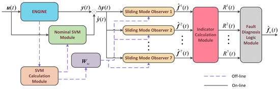
Figure 2. Robust sensor fault reconstruction using bank of sliding mode observers.

The working mechanism of fault diagnosis module is summarized as follows:

• When there is no sensor fault, each robust reconstruction ${\widehat{\mathit{f}}}_r$ has a small estimation error and indicator calculation module can also get a small scalar indicator $R$. In the diagnosis module, the sum of 7 indicators is less than the pre-defined threshold value $R_e$, indicating that no sensor fault occurs at this time.
• When there are one or more sensor faults, there will be a large error in the reconstruction generated by the observer without applying the correct assumptions, so that the corresponding indicators will be larger than those with the correct assumptions. In the fault diagnosis module, due to the occurrence of faults, the sum of all the indicators will exceed the set threshold value $R_e$, indicating there exist sensor faults. The reconstruction generated by the observer corresponding to the smallest indicator is selected as the final estimation result of the proposed architecture.

The flow chart of fault diagnosis module is shown in Figure 3:

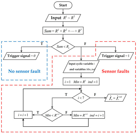
Figure 3. Flow chart of fault diagnosis module.

where ${\widehat{\mathit{f}}}_n$ is the final robust reconstruction of sensor faults, $ind$ is the index of the indicator with the minimum value, and trigger signal is aim to determine whether there is a sensor fault.

3. Application of the Method to an Aircraft Engine

A CLM of a commercial turbofan engine is used in this section. By linearizing the engine at the cruise design point ($H=\mathrm{10,668} \mathrm{m}$, $Ma=0.785$, 100% fan speed), an SVM can be obtained to characterize the engine’s small range dynamic characteristics, and observer parameters are well calculated. Simulations on CLM are carried out to examine the method in the cruise condition. To represent real working environment, the white Gaussian measurement noise and process noise are considered with variance values of 0.0015² and 0.0005² (percentage of the nominal value) [34]. The coefficient matrices are as follows:

$$\begin{array}{l}\mathit{A}=\left[\begin{array}{cc}-1.299& 1.284\\ -0.055& -1.319\end{array}\right]\mathit{B}=\left[\begin{array}{c}0.225\\ 0.188\end{array}\right]\\ \mathit{C}=\left[\begin{array}{cc}1& 0\\ 0& 1\\ 0.342& -0.154\\ 1.061& -0.522\\ 0.053& 1.518\\ 0.582& 3.012\\ -0.311& -0.962\end{array}\right]\mathit{D}=\left[\begin{array}{c}0\\ 0\\ 0.008\\ -0.005\\ 0.038\\ 0.103\\ 0.536\end{array}\right]\end{array}$$

(45)

Uncertainty $\mathit{\xi }(\mathit{x},t)$ present in this system is composed of parametric uncertainties ${\mathit{\xi }}_1\in {ℝ}^9$ and external disturbance ${\xi }_2\in {ℝ}^1$ ($\mathit{\xi }={[\begin{array}{cc}{\mathit{\xi }}_1{}^{\mathrm{T}}& {\xi }_2{}^{\mathrm{T}}\end{array}]}^{\mathrm{T}}$). The parametric uncertainty is given by:

$${\mathit{\xi }}_1(\mathit{x},t)=0.01\times \left[\begin{array}{cc}-1.299& 1.284\\ -0.055& -1.319\\ 0& 0\\ 0& 0\\ 0.342& -0.154\\ 1.061& -0.522\\ 0.053& 1.518\\ 0.582& 3.012\\ -0.311& -0.962\end{array}\right]\mathit{x}(t),$$

(46)

External disturbance is Gaussian distributed noise with mean value of 0.004 and variance value of 0.003². The distribution matrices ${\mathit{Q}}_1$ and ${\mathit{Q}}_2$ in Equations (3) and (4) are assumed to have structures given by:

$$\begin{array}{l}{\mathit{Q}}_1=\left[\begin{array}{cccccccccc}1& 0& 0& 0& 0& 0& 0& 0& 0& 1\\ 0& 1& 0& 0& 0& 0& 0& 0& 0& 1\end{array}\right]\\ {\mathit{Q}}_2=\left[\begin{array}{cccccccccc}0& 0& 1& 0& 0& 0& 0& 0& 0& 1\\ 0& 0& 0& 1& 0& 0& 0& 0& 0& 1\\ 0& 0& 0& 0& 1& 0& 0& 0& 0& 1\\ 0& 0& 0& 0& 0& 1& 0& 0& 0& 1\\ 0& 0& 0& 0& 0& 0& 1& 0& 0& 1\\ 0& 0& 0& 0& 0& 0& 0& 1& 0& 1\\ 0& 0& 0& 0& 0& 0& 0& 0& 1& 1\end{array}\right]\end{array}$$

(47)

According to the design method introduced in the previous section, the selected values of relevant design parameters are as follows:

$$\beta =0.6,\gamma =2,k_1=1.645,k_2=0.120,{\mathit{A}}_f=40{\mathit{I}}_7,R_e=0.07,$$

(48)

Taking the design of the first sliding mode observer as an example, since it is assumed that the first sensor will not malfunction, the sensor fault distribution matrix $\mathit{N}$ has the following form:

$$\mathit{N}=\left[\begin{array}{c}{\mathit{0}}_{1\times 6}\\ {\mathit{I}}_6\end{array}\right],$$

(49)

By LMI software, the design freedom ${\mathit{W}}_1\in {ℝ}^{7\times 1}$ in the scaling matrix ${\mathit{W}}_{sc}$ can be obtained as

$${\mathit{W}}_1={\left[\begin{array}{cccccc}-0.008& -0.007& -0.022& -0.014& -0.039& 0.016\end{array}\right]}^{\mathrm{T}},$$

(50)

At the engine cruise design point, four sensor fault modes are examined, covering both the hard and soft faults, and single and multiple faults, as shown in Table 2.

Table 2. Descriptions of 4 fault modes.

Mode Number	Description
Mode 1	−4% on $N_L$ at $t=5s$
Mode 2	−4% on $N_L$ over $50s$
Mode 3	−4% on $N_L$ and −6% on $T_{495}$ at $t=5s$
Mode 4	−5% on $N_L$ and −3% on $N_H$ over $50s$

Consider a scenario where all the sensors remain fault free, the comparison between threshold value $R_e$ and sum of all indicators is shown in Figure 4, which indicates no sensor fault occurred.

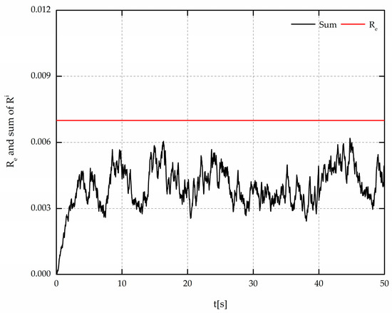
Figure 4. Comparison between threshold and sum of indicators in the case of no fault.

When the fault in Mode 1 is injected into CLM, the fault indication signals and their sum are shown in Figure 5 and Figure 6, respectively. Figure 7 shows the comparison between robust reconstruction ${\widehat{\mathit{f}}}_n$ and reconstruction $\widehat{\mathit{f}}$ without robust design in Mode 1.

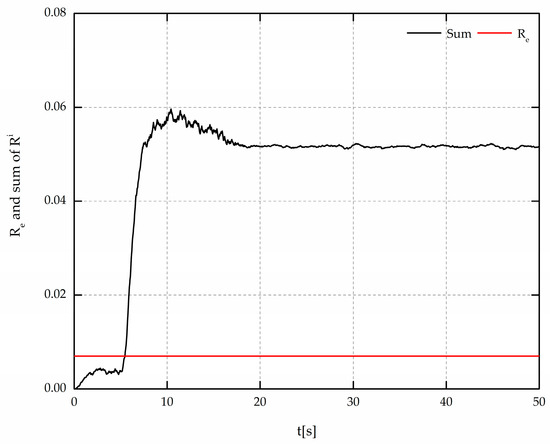
Figure 5. Comparison between threshold and sum of indicators in Mode 1.

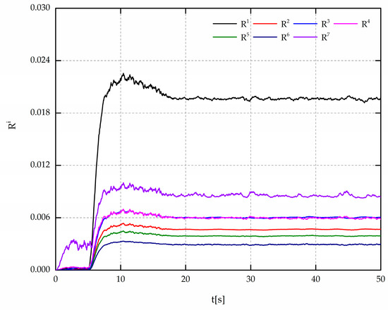
Figure 6. Fault indicator signals of the bank of SMOs in Mode 1.

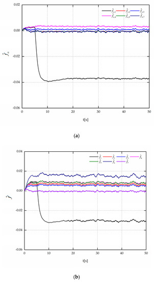
Figure 7. Sensor fault reconstruction in Mode 1: (a) Robust sensor fault reconstruction ${\widehat{\mathit{f}}}_n$; (b) reconstruction $\widehat{\mathit{f}}$ without any robust design.

From Figure 6, the fault indicator signal generated by the SMO1 is much larger than the others. This is because the fault of Mode 1 does not satisfy the assumption of SMO1, and its reconstruction shown in Figure 8 has a large estimation error. With the proposed fault diagnosis module, the sensor fault can be detected around 6 s, and the final robust reconstruction ${\widehat{\mathit{f}}}_n$ is shown in Figure 7. In the reconstruction with robust design the estimation error can be guaranteed within 0.5%, while the estimation results without robust design are relatively worse where the maximum estimation error partially reaches 1.8%.

Figure 8. Fault reconstruction generated by SMO1 in Mode 1.

To verify the effectiveness of the method under the sensor soft fault cases, Mode 2 is injected into CLM. The fault indication signals and their sum are shown in Figure 9 and Figure 10, respectively. Figure 11 shows the comparison between robust reconstruction ${\widehat{\mathit{f}}}_n$ and reconstruction $\widehat{\mathit{f}}$ without robust design in Mode 2.

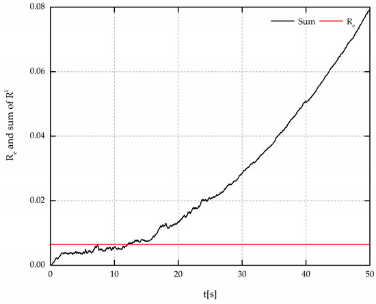
Figure 9. Comparison between threshold and sum of indicators in Mode 2.

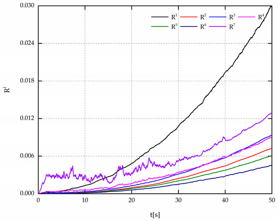
Figure 10. Fault indicator signals of the bank of SMOs in Mode 2.

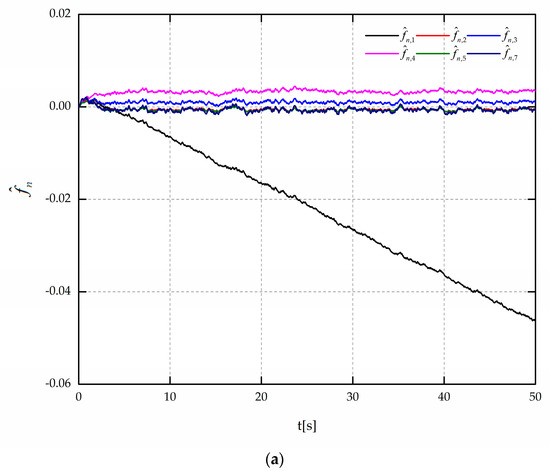
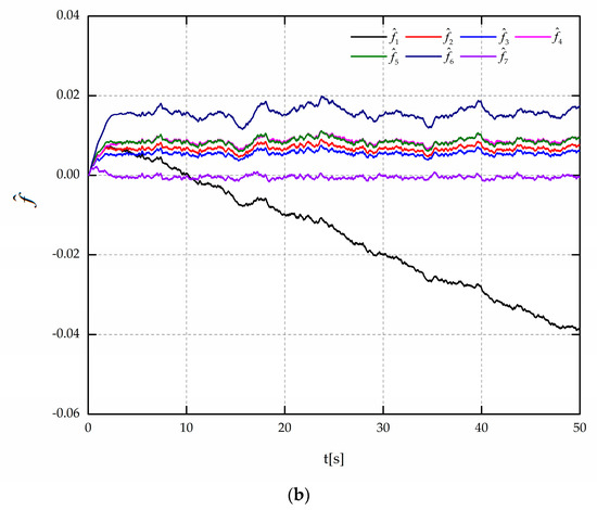
Figure 11. Sensor fault reconstruction in Mode 2: (a) Robust sensor fault reconstruction ${\widehat{\mathit{f}}}_n$; (b) reconstruction $\widehat{\mathit{f}}$ without robust design.

From Figure 11, the method proposed in this paper is still effective for sensor soft fault, reducing the influence of uncertainty on reconstruction results, and ensuring the estimation error less than 0.5%.

Mode 3 and 4 represent hard and soft faults in multi-fault cases, respectively. Figure 12 and Figure 13 show the sensor fault reconstructions in Mode 3 and 4, respectively.

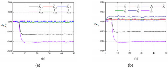
Figure 12. Sensor fault reconstruction in Mode 3: (a) Robust sensor fault reconstruction ${\widehat{\mathit{f}}}_n$; (b) reconstruction $\widehat{\mathit{f}}$ without robust design.

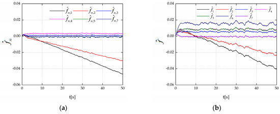
Figure 13. Sensor fault reconstruction in Mode 4: (a) Robust sensor fault reconstruction ${\widehat{\mathit{f}}}_n$; (b) reconstruction $\widehat{\mathit{f}}$ without robust design.

The effectiveness of this method is proved in the case of simultaneous faults of multiple sensors. Figure 14 shows the comparison of the maximum estimation error between the proposed robust method and the design without considering uncertainty.

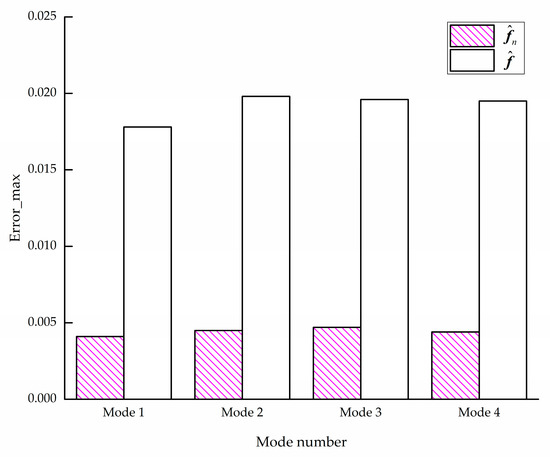
Figure 14. Maximum estimation error.

From Figure 14, the reconstruction errors can be guaranteed to be less than 0.5% for both hard and soft faults. Compared with the reconstructions without robust design, the proposed method reduces the influence of uncertainty on the reconstructions.

4. Conclusions

In this paper, a bank of second-order sliding mode observer has been designed based on the super-twisting structure for robust sensor fault reconstruction. In order to reduce the influence of uncertainties on reconstructions, the proposed method has minimized the $L_2$ gain of the transfer matrix from uncertainty to the reconstructions by designing a scaling matrix ${\mathit{W}}_{sc}$. Facing the problem of lacking design freedom in the square system, a bank of sliding mode observers has been proposed, in which each observer corresponds to a certain sensor with the assumption that the corresponding sensor would not have faults, so that the design freedom is available for robust design. When sensor faults occur, estimation errors generated by the observers with wrong hypothesis would be large. Then, through the logical diagnosis module, sensor faults can be detected and the optimal robust reconstruction results can be obtained. Numerical simulations covering diverse fault scenarios have shown the ascendency of the proposed method.

References

- Salehi, R.; Alasty, A.; Shahbakhti, M.; Vossoughi, G. Detection and isolation of faults in the exhaust path of turbocharged automotive engines. Int. J. Automot. Technol. 2015, 16, 127–138. [Google Scholar] [CrossRef]
- Dimogianopoulos, D.G.; Hios, J.D.; Fassois, S.D. Onboard Engine FDI in Autonomous Aircrafts Using Compact Stochastic Nonlinear Modelling of Flight Signal Dependencies. In Proceedings of the European Control Conference, Kos, Greece, 2–5 July 2007. [Google Scholar]
- Amozegar, M.; Khorasani, K.; Amozeghar, M. An ensemble of dynamic neural network identifiers for fault detection and isolation of gas turbine engines. Neural Netw. 2016, 76, 106–121. [Google Scholar] [CrossRef] [PubMed]
- Zhang, J.; Swain, A.K.; Nguang, S.K. Robust sliding mode observer based fault estimation for certain class of uncertain nonlinear systems. Asian J. Control 2015, 17, 1296–1309. [Google Scholar] [CrossRef]
- Simon, D.L.; Garg, S. Optimal Tuner Selection for Kalman filter-based aircraft engine performance estimation. In Printed Proceedings of the ASME Turbo Expo 2009: V. 7, Pt. A: Power for Land, Sea, and Air (GT2009), 8–12 June 2009, Orlando, FL, USA; American Society of Mechanical Engineers: New York, NY, USA, 2009; pp. 659–671. [Google Scholar]
- Feng, L.; Huang, J.Q.; Qiu, X.J. Application of multi-outputs LSSVR by PSO to the aero-engine model. J. Syst. Eng. Electron. 2009, 20, 1153–1158. [Google Scholar]
- Kobayashi, T.; Simon, D.L. Application of a Bank of Kalman Filters for Aircraft Engine Fault Diagnostics. Turbo. Expo. 2003, 1, 461–470. [Google Scholar]
- Frank, P.M. Fault diagnosis in dynamic systems using analytical and knowledge-based redundancy: A survey and some new results. Automatica 1990, 26, 459–474. [Google Scholar] [CrossRef]
- Pazera, M.; Buciakowski, M.; Witczak, M. Robust Multiple Sensor Fault–Tolerant Control for Dynamic Non–Linear Systems: Application to the Aerodynamical Twin–Rotor System. Int. J. Appl. Math. Comput. Sci. 2018, 28, 297–308. [Google Scholar] [CrossRef]
- Buciakowski, M.; Witczak, M.; Mrugalski, M.; Theilliol, D. A quadratic boundedness approach to robust DC motor fault estimation. Control Eng. Pract. 2017, 66, 181–194. [Google Scholar] [CrossRef]
- Li, J.; Park, J.H.; Ye, D. Fault detection filter design for switched systems with quantisation effects and packet dropout. IET Control Theory Appl. 2016, 11, 182–193. [Google Scholar] [CrossRef]
- Cai, J.; Ferdowsi, H.; Sarangapani, J. Model-based fault detection, estimation, and prediction for a class of linear distributed parameter systems. Automatica 2016, 66, 122–131. [Google Scholar] [CrossRef]
- Zhang, X. Sensor Bias Fault Detection and Isolation in a Class of Nonlinear Uncertain Systems Using Adaptive Estimation. IEEE Trans. Autom. Control 2011, 56, 1220–1226. [Google Scholar] [CrossRef]
- Jiang, B.; Staroswiecki, M.; Cocquempot, V. Fault Accommodation for Nonlinear Dynamic Systems. IEEE Trans. Autom. Control 2006, 51, 1578–1583. [Google Scholar] [CrossRef]
- Chen, J.; Patton, R.J. Robust Model-Based Fault Diagnosis for Dynamic Systems; Springer Science & Business Media: Berlin, Germany, 2012; Volume 3. [Google Scholar]
- Liu, M.; Zhang, L.; Shi, P.; Karimi, H.R. Robust Control of Stochastic Systems Against Bounded Disturbances with Application to Flight Control. IEEE Trans. Ind. Electron. 2014, 61, 1504–1515. [Google Scholar] [CrossRef]
- Alwi, H.; Edwards, C.; Tan, C.P. Fault Detection and Fault-Tolerant Control. Using Sliding Modes; Springer: London, UK, 2011. [Google Scholar]
- Liu, M.; Shi, P. Sensor fault estimation and tolerant control for Itô stochastic systems with a descriptor sliding mode approach. Automatica. 2013, 49, 1242–1250. [Google Scholar] [CrossRef]
- Tan, C.P.; Edwards, C. Sliding mode observers for detection and reconstruction of sensor faults. Automatica 2002, 38, 1815–1821. [Google Scholar] [CrossRef]
- Bouibed, K.; Seddiki, L.; Guelton, K.; Akdag, H. Actuator fault detection by nonlinear sliding mode observers: Application to an actuated seat, 2013. In Proceedings of the Conference on Control and Fault-Tolerant Systems (SysTol), Nice, France, 9–11 October 2013; pp. 739–743. [Google Scholar]
- Yan, X.G.; Edwards, C. Robust sliding mode observer-based actuator fault detection and isolation for a class of nonlinear systems. Int. J. Syst. Sci. 2008, 39, 349–359. [Google Scholar] [CrossRef]
- Chang, X.; Huang, J.; Lu, F. Health Parameter Estimation with Second-Order Sliding Mode Observer for a Turbofan Engine. Energies 2017, 10, 1040. [Google Scholar] [CrossRef]
- Laghrouche, S.; Liu, J.; Ahmed, F.S.; Harmouche, M.; Wack, M. Adaptive Second-Order Sliding Mode Observer-Based Fault Reconstruction for PEM Fuel Cell Air-Feed System. IEEE Trans. Control Syst. Technol. 2015, 23, 1098–1109. [Google Scholar] [CrossRef]
- Levant, A. Quasi-continuous high-order sliding-mode controllers. In Proceedings of the 42nd IEEE International Conference on Decision and Control, Maui, HI, USA, 9–12 December 2003; pp. 4605–4610. [Google Scholar]
- Levant, A.J. Principles of 2-sliding mode design. Automatica 2007, 43, 576–586. [Google Scholar] [CrossRef]
- Levant, A. Sliding order and sliding accuracy in sliding mode control. Int. J. Control 1993, 58, 1247–1263. [Google Scholar] [CrossRef]
- Moreno, J.A.; Osorio, M. A Lyapunov approach to second-order sliding mode controllers and observers. In Proceedings of the 47th IEEE Conference on Decision and Control, Cancun, Mexico, 9–11 December 2008; pp. 2856–2861. [Google Scholar]
- Moreno, J.A.; Osorio, M. Strict Lyapunov Functions for the Super-Twisting Algorithm. IEEE Trans. Autom. Control 2012, 57, 1035–1040. [Google Scholar] [CrossRef]
- Ben Brahim, A.; Dhahri, S.; Ben Hmida, F.; Sellami, A. Simultaneous actuator and sensor faults reconstruction based on robust sliding mode observer for a class of nonlinear systems. Asian J. Control 2017, 19, 362–371. [Google Scholar] [CrossRef]
- Alaei, H.K.; Yazdizadeh, A. Robust Output Disturbance, Actuator and Sensor Faults Reconstruction Using H∞ Sliding Mode Descriptor Observer for Uncertain Nonlinear Boiler System. Int. J. Control Autom. Syst. 2018, 16, 1271–1281. [Google Scholar] [CrossRef]
- Zhao, K.; Li, P.; Zhang, C.; Li, X.; He, J.; Lin, Y. Sliding Mode Observer-Based Current Sensor Fault Reconstruction and Unknown Load Disturbance Estimation for PMSM Driven System. Sensors 2017, 17, 2833. [Google Scholar] [CrossRef] [PubMed]
- Buciakowski, M.; Pazera, M.; Witczak, M. A Combined H2/H∞ Approach for Robust Joint Actuator and Sensor Fault Estimation: Application to a DC Servo-Motor System. Sensors 2019, 19, 2648. [Google Scholar] [CrossRef] [PubMed]
- Tan, C.P.; Edwards, C. An LMI approach for designing sliding mode observers. Int. J. Control 2001, 74, 1559–1568. [Google Scholar] [CrossRef]
- Lu, F.; Huang, J.; Lv, Y. Gas Path Health Monitoring for a Turbofan Engine Based on a Nonlinear Filtering Approach. Energies 2013, 6, 492–513. [Google Scholar] [CrossRef]
© 2019 by the authors. Licensee MDPI, Basel, Switzerland. This article is an open access article distributed under the terms and conditions of the Creative Commons Attribution (CC BY) license (http://creativecommons.org/licenses/by/4.0/).