Abstract
The formation of pollutant emissions in jet engines is closely related to the fuel distribution inside the combustor. Hence, the characteristics of the spray formed during primary breakup are of major importance for an accurate prediction of the pollutant emissions. Currently, an Euler–Lagrangian approach for droplet transport in combination with combustion and pollutant formation models is used to predict the pollutant emissions. The missing element for predicting these emissions more accurately is well defined starting conditions for the liquid fuel droplets as they emerge from the fuel nozzle. Recently, it was demonstrated that the primary breakup can be predicted from first principles by the Lagrangian, mesh-free, Smoothed Particle Hydrodynamics (SPH) method. In the present work, 2D Direct Numerical Simulations (DNS) of a planar prefilming airblast atomizer using the SPH method are presented, which capture most of the breakup phenomena known from experiments. Strong links between the ligament breakup and the resulting spray in terms of droplet size, trajectory and velocity are demonstrated. The SPH predictions at elevated pressure conditions resemble quite well the effects observed in experiments. Significant interdependencies between droplet diameter, position and velocity are observed. This encourages to employ such multidimensional interdependence relations as a base for the development of primary atomization models.
1. Introduction
The design of aircraft propulsion systems, mainly gas turbines, is facing major challenges regarding the reduction of noise, pollutants and greenhouse gas emissions. The combustion chamber of a jet engine is the key component to meet these requirements. The design process of combustion chambers strongly relies on numerical methods, mostly Euler–Lagrangian simulations of the reacting spray. Combined with models for fuel injection, turbulent dispersion, secondary breakup and evaporation of droplets as well as models for combustion and pollutant formation, this approach enables the numerical prediction of pollutant emissions. Besides the air distribution, pressure, temperature and other parameters, the fuel atomization and the resulting spray have a significant influence on the pollutant formation processes [1]. Hence, the reliable prediction of pollutant emissions strongly depends on the precise prediction of the droplet trajectory through the combustion chamber, which is influenced by its starting conditions and the airflow through the atomizer [1]. The interaction of air and fuel droplets can be captured by the momentum equation [2]. In recent Euler–Lagrangian simulations of aero-engine combustion chambers, different methodologies have been used to set the droplet starting conditions. The initial droplet diameters are usually computed using drop size distributions [3,4,5,6,7,8,9], which are derived by primary atomization models. Those correlations are mostly derived from measurements downstream from the injection location. Due to the annular shape of the injector nozzle, the droplets are assumed to be injected at multiple discrete injection points equally distributed on a circle [6,8]. The position of the circle downstream from the injector nozzle is selected to fit experimental data. Usually, the initial droplet velocity is purely axial, neglecting the radial and tangential components. Some authors set a fixed initial axial velocity [4,5,7,8], while others use models to predict the initial axial velocity depending on the droplet diameter [3,6].
These common definitions of the droplet starting position and the initial velocity vector are illustrated in Figure 1.
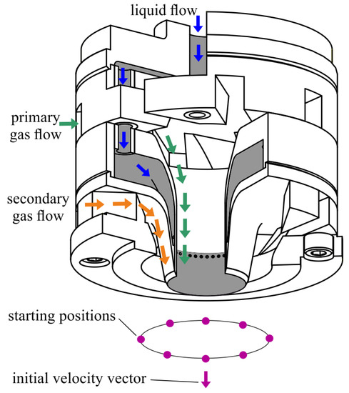
Figure 1.
Sketch of annular prefilming airblast nozzle illustrating common droplet starting positions and initial velocity vector in magenta, adapted from [10].
In most publications the initial diameter, position and velocity are treated independently, and sometimes a relation between droplet size and axial velocity is considered. Consequently, there is a lack of knowledge if and how droplet diameter, position and velocity are correlated.
Collecting such data for elevated pressure conditions and for realistic injector geometries may be quite challenging, due to complex experimental facilities and restricted optical access. Hence, some attempts have been made to predict the atomization process numerically from first principles. In the context of prefilming airblast atomization, Euler–Euler [11,12,13] and Lagrange–Lagrange [14] approaches have been developed to resolve the gas–liquid interface. Two-phase simulations at elevated pressure have been conducted using both fully Eulerian methods [12] as well as fully Lagrangian methods [15].
In the present work, the fully Lagrangian Smoothed Particle Hydrodynamics (SPH) method is applied for simulating the breakup process of a prefilming airblast atomizer with different trailing edge thicknesses and gas velocities. The main objectives of this study are (i) to provide spray characteristics close to the fuel nozzle and at elevated pressure, (ii) to analyse breakup and spray quantities using descriptive statistics, (iii) to explain relations between ligament breakup and spray formation, (iv) to highlight the multivariate interdependencies between the spray quantities, (v) to show the effects of trailing edge thickness and gas velocity on these multivariate interdependencies within the sprays, (vi) to give detailed statistical insights into the ligament and spray formation, which support the selection of appropriate modelling methods. The paper is organized as follows. First, the numerical method is introduced. Second, the investigated atomizer geometry and operating conditions as well as the details of the numerical setup are presented. Third, the characteristic quantities and the sampling procedure are introduced. Fourth, the airflow field around the prefilmer is described. Then the breakup phenomena as well as the resulting ligament and spray quantities including the multivariate interdependencies between each other are discussed for one baseline case. Subsequently, the effects of trailing edge thickness and gas velocity on these multivariate interdependencies are outlined. Finally, the impact of the present work on modelling primary atomization is discussed.
2. Numerical Method
The Smoothed Particle Hydrodynamics (SPH) method is a mesh-free method that relies on a Lagrangian representation of the fluid by particles moving with the velocity of the fluid. The particles carry the physical properties of the fluid such as mass, momentum and energy. This method was originally developed for astrophysics [16,17] and later adapted to free surface flow applications [18]. In recent years, the SPH method has been applied to air-assisted liquid atomization [14,19,20].
The main advantage of the SPH method in the context of non-miscible multiphase flows is the natural handling of the phase interface. In contrast to Eulerian methods, neither an interface reconstruction nor a threshold for the volume fraction [11] are required. Furthermore, the usage of discrete particles avoids interface diffusion and enables inherent mass conservation.
Since the state of a certain particle depends on its adjacent particles, a weighting function W [18] as depicted in Figure 2 (top) is used to evaluate a function f at the particle location by:
where is the volume of the neighbour particles b, located inside the sphere of influence of particle a, as illustrated in Figure 2 (bottom).
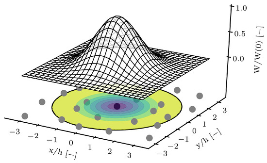
Figure 2.
Top: Illustration of a 2D kernel. Bottom: Particle distribution superimposed with the kernel weight and illustration of the sphere of influence.
The weighting function is defined on a compact support, the so-called ‘sphere of influence’, that depends on the smoothing length h, and must fulfil mathematical properties such as the unity integral () and the convergence to the Dirac -function for . The Wendland kernel function [21] is used with where is the mean particle spacing.
With this formalism the Navier-Stokes equations can be cast into an SPH formulation, as explained in [14]. To close the system, the Tait equation of state is used. This approach is referred to as Weakly Compressible SPH [22]. Surface tension is applied using the Continuum Surface Force (CSF) method [23,24]. The liquid–wall interaction (contact angle) is modelled by a correction of the normal vector in the framework of the CSF model [25].
The numerical performance of the SPH code developed at the Institut für Thermische Strömungsmaschinen (ITS) has been demonstrated recently [26]. A 3D SPH simulation with this code has proved the capability of the SPH method to predict the primary breakup process accurately compared to experimental data [14,26], in particular the drop size. Using 2D SPH simulations of the primary breakup at ambient pressure, the effect of the trailing edge thickness on the atomization process has been clarified [27]. 2D SPH simulations of a realistic fuel injector geometry at high pressure conditions [28] gave detailed insights into the film flow development, mixing and spray characteristics. Consequently, the SPH method seems to be an appropriate tool for capturing the atomization process at elevated pressure.
3. Numerical Setup
In this chapter, a brief introduction to the investigated geometry and operating conditions is given. Furthermore, the details of the numerical setup with respect to the SPH method are presented.
3.1. Investigated Fuel Injector
A planar prefilming airblast atomizer, Figure 3 (left), which has been extensively studied experimentally [11,29,30], is investigated numerically using a 2D segment at the trailing edge, as depicted in Figure 3 (right). The trailing edge thickness , which has a significant influence on the generated spray [31], is set to 230 and 640 μm. Any other dimension is kept constant in this study.
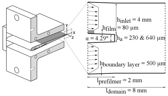
Figure 3.
Experimentally investigated prefilmer (left) and corresponding computational domain (right).
3.2. Investigated Operating Conditions
In order to consider real engine conditions, the air is assumed to be compressed isentropically from ambient conditions to a pressure of 5 bar before entering the atomizer. The air is at 464 K with a density of kg/m3 and a viscosity of 2.575 × 10 kg/m/s. The air velocity is chosen to be 70 and 90 /. As liquid, the fuel substitute Shellsol D70 is used [30]. The liquid properties of D70 are almost identical to those of kerosene, namely density = 770 kg/m, surface tension = 0.0275 kg/s and dynamic viscosity = 0.00156 kg/m/s at ambient conditions. The same liquid properties are used for all three simulations. Due to the short residence time of the liquid on the prefilmer, the liquid is assumed not to be heated up significantly. The liquid film loading is kept constant at = 75 mm/s. This is equivalent to an inlet velocity of u = 0.9375 m/s at a film height of h = 80 μm.
All three cases presented in this paper and the corresponding non-dimensional quantities are given in Table 1. The definitions can be found in Appendix A.

Table 1.
Non-dimensional quantities describing prefilming airblast atomization (c.f. Appendix A).
3.3. Details of the SPH Setup
The 2D domain is discretized by three different types of particles representing the air, the fuel and the walls. In previous simulations (page 4 in [27]), the influence of the mean particle distance, i.e., the spatial resolution on the airflow field and the spray, was studied at ambient conditions and at a medium air velocity ( = 50 m/s). From these simulations it was concluded that a mean particle distance of 5 μm is a good compromise between accuracy and computational effort. For the simulations presented in this paper the mean particle distance has been reduced to μm, since elevated air pressure ( = 5 bar) and high air velocity ( = 90 m/s) are covered. This fine spatial resolution is required for capturing the atomization process properly. It results into 11.3 Mio particles within the domain. Due to an adaptive time stepping which takes into account the Courant–Friedrichs–Lewy (CFL) condition and the maximum acceleration as well as viscous effects and surface tension, the mean step time varies between 64 and 68 .
No turbulence model has been applied. The smallest turbulence length and time scales can be estimated using the channel height of 8.11 mm [30] as large scale, a turbulence intensity of 10 [30] and taking into account the variation of air velocity. This results into Kolmogorov length scales from 6.7 to 8 μm and Kolmogorov time scales of 6.4 to μs (Table 1 in [32]). Hence, the smallest turbulence scales in time and space are adequately resolved by the present simulations, meaning Direct Numerical Simulations (DNS) are conducted.
In the Tait equation of state, the polytropic exponent is taken as 7 and the fictive speed of sound are m/s for the air and m/s for the liquid fuel. The background pressure is set to bar. The contact angle of the wall–liquid–gas interface is kept constant at an angle of 60°.
Using 1000 CPUs for 72 h for each simulation, 511 to 633 through flow times were simulated.
4. Results and Discussion
4.1. Characteristic Quantities and Sampling Procedure
The ligament breakup can be characterized using five quantities as illustrated in Figure 4. The SPH particles which form the liquid structure attached to the trailing edge (red and green) are identified using a Connected Component Labeling technique [33]. The liquid on the prefilmer (red) is neglected in the following analysis. A length scale characterizing the size of the ligament (green) is derived from the equivalent area of a circle. The size of the ligament in stream-wise direction is equal to its projected length from the trailing edge to its maximum x-coordinate. The height of the ligament is defined by the difference between the minimal and maximal y-coordinates of the ligament. The axial and vertical velocity of the ligament and are obtained at the crest of the ligament. The crest is defined by the particle of the ligament with the maximum x-coordinate.
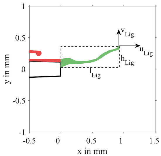
Figure 4.
Quantities describing the ligament breakup.
To investigate the spray quantitatively, clusters of liquid particles are identified using a Connected Component Labeling technique [33]. Each particle cluster with 5 or more particles is considered to represent a droplet. The droplet diameter is determined by the equivalent area of a circle. These two assumptions lead to a minimum detectable diameter of μm. The centroid of the clustered particles is assumed to represents the droplet positions and . The droplet velocities and are equivalent to the mean velocities of all particles representing the cluster. Furthermore, only droplets located downstream from the trailing edge and which do not touch the top and bottom walls are taken into account. In the present work, the droplet set of each operating point comprises the droplets of all time steps and consists of 137,000 to 243,000 droplets. Due to the high sampling frequency, most droplets are taken into account multiple times during their flight through the domain. Since no recirculation zone is established in the airflow field (Figure 5), the droplets will move towards the outlet to the domain. Droplets hitting the top and bottom wall boundaries of the computational domain are removed from the further analysis by filtering ( 4 mm).
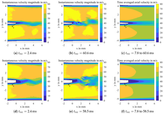
Figure 5.
Instantaneous and time averaged airflow field for = 5 bar, = 70 /, = 230 and 640 μm.
4.2. Airflow Field
The prefilming airblast atomization is driven by the momentum transfer from the airflow to the liquid fuel. The airflow around and downstream from the trailing edge is presented in Figure 5 using both the instantaneous velocity magnitude as well as the time averaged axial velocity.
Two instantaneous flow fields are recorded ms after the start of the simulation, which is ms after the first droplets are formed downstream from the prefilmer (Figure 5a,d). Two more instantaneous flow fields are recorded at the end of the simulations (Figure 5b,e). The time averaged flow fields are obtained from ms to ms and ms, respectively (Figure 5c,f). Hence, for all plots, the prefilmer is wetted and liquid undergoes breakup. It is clearly visible that vortex shedding occurs downstream from the trailing edge (Figure 5a,b,d,e). As expected, the size of the wake downstream from the prefilmer is proportional to the height of the trailing edge (Figure 5c,f). Due to the liquid breakup, no recirculation zone is established.
4.3. Phenomena Observed During Breakup
Five snapshots of a breakup sequence are depicted in Figure 6 (bottom), including the recording time of the snapshots (top). Please note that a video of this breakup sequence is available online in the Supplementary Materials of this paper. In this sequence the film waves (i), the temporal evolution of one ligament (iii) as well as its breakup (iv) and finally the dispersion of the resulting droplets (v) can be observed. Due to the wavy film, most liquid is advected within the film waves (i) to the trailing edge (ii). The volume of the wave is either integrated into the liquid accumulated at the trailing edge or the wave has enough momentum to stretch out the accumulated liquid resulting in the formation of a ligament. In most cases, the tip of the ligament (Snapshot 1) reaches into the co-flowing high speed air. This causes a breaking up of the tip and a forcing of the middle part of the ligament to evade into the wake of the trailing edge. Consequently, the ligament is stretched in both the axial and vertical direction, whereas the tip mostly moves only in axial direction (Snapshots 2 and 3). The middle part dips into the lower high speed airflow (Snapshots 2 and 3). This results in the breakup of the tip and the middle part of the ligament (Snapshot 4). The resulting larger liquid structures will disintegrate further into droplets that are widely spread in the vertical direction (Snapshot 5). Meanwhile, the shortened ligament moves upwards, where it is further disintegrated by the upper airflow. This sequence will be repeated with the following film wave reaching the trailing edge (Snapshot 5).
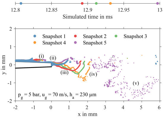
Figure 6.
Breakup sequence at the prefilmer (bottom) and recording times of snapshots (top).
Shadowgraphy images of the liquid breakup at the tip of a prefilming airblast atomizer, as studied by Gepperth et al. [11,29,30], are depicted in Figure 7. The geometry is identical to that depicted in Figure 3 (left). The side view perspective on the tip of the prefilmer is presented in the first and third column and corresponds to the sequence shown in Figure 6. The green lines represent the tip of the prefilmer. The images showing the side view are blurry since the depth of field of the camera is very small compared to the width of the wetted prefilmer (|z| ≤ 25 mm). Consequently, the liquid on the prefilmer and the liquid structures attached to the trailing edge are superimposed by each other.
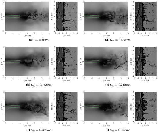
Figure 7.
Shadowgraphy images of the liquid breakup at the prefilmer tip in side view perspective (first and third column) and top view perspective (second and fourth column) for = 1 bar, = 70 /, = 230 μm, = 25 mm/s
The corresponding top view perspective of the prefilmer is presented in the second and fourth column. From the top view perspective, a wavy film flow, the accumulation of liquid at the trailing edge, the elongation of ligaments and formation of liquid bags with a thick rim and a thin interior lamella as well as their breakup can be observed. These processes are classified as primary atomization. Furthermore, the subsequent breakup of non-spherical liquid blobs into spherical droplets is depicted, which corresponds to secondary atomization. In the side view perspective the stretching, flapping and breakup of both the ligaments as well as the bags can be observed.
Please note that the shadowgraphy images correspond to operating conditions of = 1 bar, = 70 /, = 230 μm and = 25 mm/s. Compared to the results of the simulation as presented in Figure 6 only two out of four boundary conditions are met by the shadowgraphy images. This can be explained as follows: First, at higher pressure ( = 5 bar) and higher film loading ( = 75 mm/s) the number of concurrent breakup events and the amount of liquid present at the trailing edge increases rapidly. Hence, the side view perspective would not provide sufficient insights. Second, images at these conditions are not available. Since the underlying atomization mechanisms are the same for both ambient and elevated pressure, the same phenomena can be observed during breakup. Please note that experiments at low air velocity ( = 20 /) provide many insights in the side view perspective (Figure 4 in [34]). The present numerical observations are in good agreement with the experimental observations. Despite the fact that the present SPH simulations are 2D, most of these effects can be reproduced. In the following we focus on the statistical analysis of the resulting ligaments and droplets and not on the formation process itself. The dynamics of the primary breakup process have been investigated in a previous study [35].
4.4. Analysis of the Ligament Evolution
The evolution of multiple ligaments can be analysed using bivariate histograms. In Figure 8a the interdependencies between the ligament length and height are depicted.
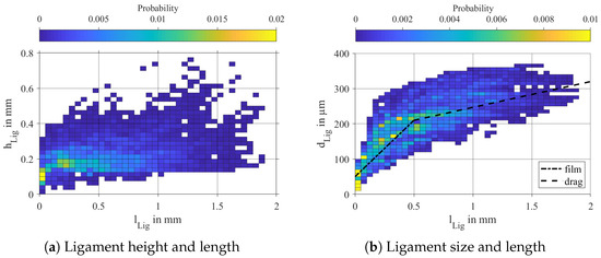
Figure 8.
Interdependencies between ligament length scales for = 5 bar, = 70 /, = 230 μm.
As the full temporal evolution from minimum to maximum elongation is covered by the data, most of the detected ligaments are smaller than mm in height and 1 mm in length. In the following discussion, ligaments smaller than mm in length are ignored, as they represent the liquid accumulated at the trailing edge instead of a ligament. Generally, the length to height ratio ranges from 1 to 10, which is reasonable due to the drag force imposed by the co-flowing air. Ligament heights mm are very unlikely to occur. This value is larger than due to the boundary layer which is established on the prefilmer (Figure 5a).
The interdependency of ligament length and ligament size is presented in Figure 8b. It can be divided into two sections using two lines. One with a steep slope (dash–dot line) and one with a flat slope (dashed line). In the first section the evolution of the ligament is dominated by the film waves. Consequently, , which is based on the area or “volume” represented by the liquid, strongly increases. In the latter section the stretching of the ligament caused by the drag force of the co-flowing air dominates. Hence, strongly increases, whereas changes only moderately.
The relation between the axial velocity of the crest of the ligament and its length is depicted in Figure 9a. Obviously, the crest velocity increases with increasing . This is reasonable since the probability of the ligament to flap and dive into the high speed airflow increases with increasing . Due to the drag forces the crest is accelerated. These findings are supported by the positive relation between and (Figure 9b). Furthermore, it can be observed that only a few events with 7 m/s occur. These result from events where the tip of the ligament is accelerated strongly by the drag forces and evades into the wake of the main part of the ligament. The negative axial crest velocities result from the contraction of the remaining ligament back to the trailing edge.
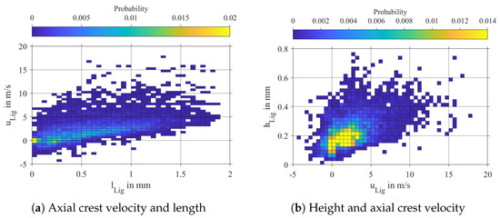
Figure 9.
Interdependencies between axial crest velocity and ligament length scales for = 5 bar, = 70 /, = 230 μm.
The vertical crest velocity is symmetrically distributed around zero with a slight trend to negative velocities as depicted in Figure 10a. With increasing no significant change can be observed, indicating that the flapping mechanism of the ligaments is independent of their length. In a previous numerical study [36] it has been observed that the vortex shedding frequencies of the airflow are at least one order of magnitude higher than the flapping frequencies of the ligaments attached to the trailing edge. However, the dynamics of gas and liquid are not part of the present work. The relation between axial and vertical crest velocity is depicted in Figure 10b. While the remaining ligament contracts back to the trailing edge ( 0 m/s), the ligaments flap vertically, resulting in both positive and negative . The ratio of axial to vertical crest velocity ranges from 2 to 20, which is reasonable due to the high speed airflow.
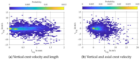
Figure 10.
Interdependencies of the vertical crest velocity for = 5 bar, = 70 /, = 230 μm.
In summary, the evolution of the ligaments is based on two mechanisms: The ligament growth driven by the film waves and the stretching of the ligaments by the drag imposed. For the investigated operating point, the acceleration of the crest of the ligament is mainly induced by drag forces. Furthermore, flapping of ligaments is observed for all ligament lengths.
4.5. Relations between Ligaments and Droplets
In the following, the interaction of ligaments and droplets is discussed using histograms of both ligament and droplet quantities (blue and orange bins). The number distributions of the ligament length and the axial position of the droplets are depicted in Figure 11a. The probability for mm is quasi constant (solid line) and then decreases linearly with a steep and flat slope (dashed line). The first region (solid line) is related to the accumulation of liquid at the trailing edge and the ligament growth. The latter region (dashed line) is a consequence of the ligament stretching and breakup (Figure 6). A characteristic length of the ligaments at breakup cannot be provided since for the simulated time too few breakup events occur. However, the probability of the presence of a drop increases asymptotically from 0 to mm and then decreases slightly. The presence of droplets in the first region (solid line) can be related to stripping phenomena where some droplets are sheered off from smaller ligaments or film waves. Longer ligaments break up fully or partially, releasing a significant number of droplets. As most of these droplets are too large to withstand the harsh airflow, subsequent breakup into smaller droplets occurs, which results in the increase of the probability from 2.0 to mm. The slight decrease of the probability more downstream is related to the different axial velocities of the droplets. These observations regarding the distributions of and are in good agreement with experimental results (Figure 29 in [29]).
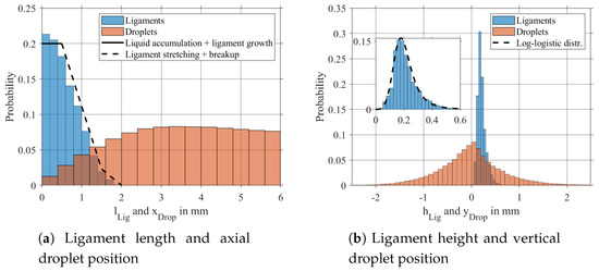
Figure 11.
Ligament length scales and droplet positions for = 5 bar, = 70 /, = 230 μm.
The probability of the projected heights of the ligaments as well as the vertical droplet positions are depicted in Figure 11b. The ligament height follows a Log-logistic distribution within 0 to 0.6 mm. This reflects the flapping mechanism of the prefilmer. Large ligaments reach into the co-flowing air and are disrupted (Figure 6). The resulting droplets are normally distributed in the vertical direction. They are more spread than the ligament crests due to the interaction with the airflow, as to be discussed later.
The amount of liquid contained in the ligaments and droplets can be analysed by using the number distribution of the ligament size and the droplet diameter , as depicted in Figure 12, since both quantities are derived from the area of the ligaments and droplets. The dimension of the ligaments is smaller than 400 μm with a peak at 235 μm following approximately a Gaussian distribution with a tail at smaller sizes. The tail results from the fact that the crest of the smaller ligaments is moving slower than the crest of large ligaments (Figure 8b and Figure 9a). Consequently, small ligaments are recorded more often than large ligaments. The largest recorded droplet is about 200 μm. The droplet size distribution shows the typical peak at small diameters and an exponential decline to larger diameters as is expected for the atomization processes. In general, both distributions reflect the disintegration of very large ligaments into much smaller droplets.
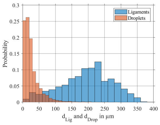
Figure 12.
Ligament size and droplet diameter for = 5 bar, = 70 /, = 230 μm.
The sprays generated by the simulations are compared to the corresponding experiment using the Sauter Mean Diameter. As the full temporal evolution of the droplets is captured by the simulations, slowly moving droplets are taken into account more often than fast moving droplets. This bias is counterbalanced by a weight based on the droplet velocity (page 77 in [19]). It is defined as . The length scale l is equal to the length of the sampling region ( mm) and the time scale is the median between all saved snapshots of one simulation. Thus, the velocity weighted SMD can be defined as: . The experimental are derived from an experimental correlation which is based on non-dimensional quantities (Appendix B). The resulting SMDs are presented in Table 2. For all three cases, a good agreement between the numerical results and the experimental correlation can be observed. Thus, the trends indicated by the correlation can be reproduced very well by the simulations.
Table 2.
Sauter Mean Diameters of Smoothed Particle Hydrodynamics (SPH) simulations and experimental correlation.
The velocity distributions of the crest of the ligament and the resulting droplets are presented in Figure 13. The axial crest velocity (Figure 13a) follows approximately a Gaussian distribution with a tail at high velocities. A peak is observed at / and negative velocities up to /. Negative axial crest velocities can be triggered by the flapping of the ligaments around the trailing edge when its size is not changed and by the contraction of the ligaments after breakup. The maximum crest velocity is about 15 / and much smaller than the bulk velocity of the gas ( = 70 /). In contrast, the maximum axial velocity of the droplets is 76 / and thus even higher than . This is reasonable, since by the flapping ligament the effective channel height is reduced when it reaches into the airflow (Figure 6). Consequently, the airflow is locally accelerated. The distribution of is bimodal and can be represented by two Gaussian distributions with peaks at / and 30 /. The Gaussian distribution at the slower velocities (dashed line) represents the droplets that are generated directly after the disintegration from the ligament crest. Hence, the range of m/s is fully covered by . The Gaussian distribution at the faster velocities (dash–dot line) corresponds to the droplets that are accelerated by the fast co-flowing air. This bimodal character of the distribution was also observed in experiments (Figure 33 in [29]).
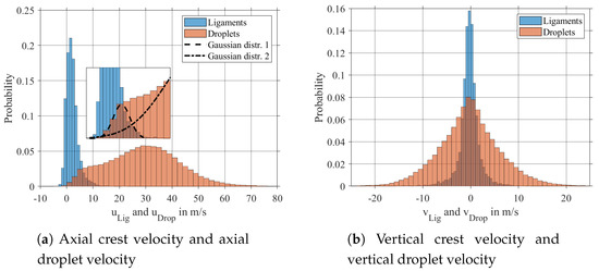
Figure 13.
Velocities of ligament crest and droplets for = 5 bar, = 70 /, = 230 μm.
The vertical velocities of ligament crest and droplets are depicted in Figure 13b. Both follow a Gaussian distribution. However, the distribution of is much broader than that of . When the crests of the ligaments dive into the fast co-flowing air, their movement in vertical direction is slowed down due to the drag force imposed by the airflow on the body of the ligament (Figure 6). Immediately after the detachment from the ligament, the droplet is no more pulled down by the ligament. Hence, they can move faster than the ligament crest.
As to be expected, the ligaments and the droplets immediately after breakup are closely related, for example, in terms of axial velocity. However, the longer a droplet exist, the more its movement is influenced by the drag forces imposed by the co-flowing air.
4.6. Analysis of the Spray Evolution
The marginal distributions of the droplet quantities, as discussed in the previous section, revealed several interdependencies between these quantities. These can be further analysed using bivariate histograms which represent the joint probability. In Figure 14a the joint probability between droplet diameter and its axial position downstream from the trailing edge is depicted. This plot can be interpreted as the evolution of the droplet size distribution over time. A primary breakup zone ( mm) and a secondary breakup zone ( mm) can be identified. The primary breakup zone is characterized by large droplets ( 100 μm) and is superimposed by the ligament breakup (Figure 11a). These large droplets will break up into smaller ones. Consequently, the number of small droplets will increase in the secondary breakup zone, whereas the number of large droplets will decrease.
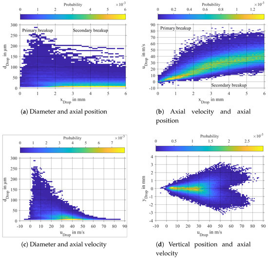
Figure 14.
Interdependencies of spray quantities for = 5 bar, = 70 /, = 230 μm.
The velocity of the droplets in the streamwise direction is illustrated by Figure 14b. Within the primary breakup zone most of the droplets move rather slow, m/s, which is in the same range as the ligament crest velocities as presented in Figure 13a. Furthermore, the velocity distribution becomes significantly broader, because existing droplets are accelerated, while actually generated droplets have the same velocity as the crest of the ligament. In the secondary breakup zone most of the droplets are accelerated to up to 50 /. The maximum speed of a droplet depends on its size as depicted in Figure 14c, where the relation between the axial droplet velocity and the droplet diameter is presented. It can be observed that the maximum speed of a droplet is inverse proportional to its size. Large droplets ( 100 μm) experience a significant amount of drag force, but as the inertia dominates, the relative velocity remains high, resulting in the breakup of these droplets. Consequently, these droplets cannot reach high velocities ( m/s). The resulting smaller droplets and the already existing ones can handle the acceleration better. Thus, these reach higher velocities. The maximum axial droplet velocity increases with , which is in good agreement with experimental and numerical investigations (Figure 26 in [11]).
The structure of the airflow field (Figure 5) strongly influences the relation between axial droplet velocity and the vertical droplet position as presented in Figure 14d. Most of the droplets remain in the wake of the prefilmer (200 μm), where they reach velocities of 30 to 60 m/s. Droplets entering the co-flowing air get significantly faster ( m/s). The minimum velocity of the droplets increases linearly with increasing distance from the prefilmer. As all droplets entering the high speed airflow move from the inner to the outer region of the computational domain (increasing ), Figure 14d represents the acceleration of these droplets over time by the airflow.
The relations between the droplet diameter and both the vertical droplet position and velocity are depicted in Figure 15a,b. Both quantities follow a Gaussian distribution around zero and their width is inversely proportional to the droplet size. Large droplets ( 100 μm) can only exist in and close to the wake downstream from the prefilmer ( mm). Thus, their vertical velocity m/s is relatively small.
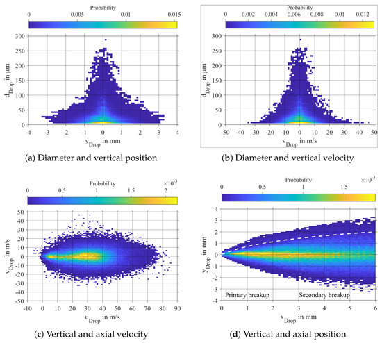
Figure 15.
Interdependencies of spray quantities for = 5 bar, = 70 /, = 230 μm.
It is actually the same range as the vertical velocities of the crest of the ligaments (Figure 13b). The smaller droplets are expelled into the fast co-flowing air ( mm) and reach higher vertical velocities ( m/s). The resulting droplet velocity vectors are depicted in Figure 15c. The ratio ranges from 0.5 to 80. However, for most of the droplets, the axial component dominates. These vectors are related to the droplet trajectories as depicted in Figure 15d. The droplets are widely spread over the domain, forming a typical spray cone. Usually their trajectory follows a parabolic curve (dashed line). Some droplets cross the domain from top to bottom and vice versa, resulting in more chaotic trajectories. In summary, strong relations between all droplet quantities, namely diameter, position and velocity, are observed in the presented data. Hence, the correct representation of the spray characteristics near the injector is required, for example, for simulations focusing on soot production [37]. Consequently, the multivariate interdependencies of the spray quantities as outlined previously have to be taken into account.
4.7. Effect of Gas Velocity and Prefilmer Geometry on the Spray Evolution
In this section the effect of gas velocity and the trailing edge thickness of the prefilmer on the interdependencies within the spray are outlined. Therefore, the kernel densities corresponding to Figure 14 and Figure 15 are estimated and analysed using lines of constant probability (isolines). For the baseline case ( = 5 bar, = 70 /, = 230 μm) up to three different isolines are plotted in red to illustrate the bivariate distribution. The value of the isolines are indicated by corresponding labels. For the cases to be compared ( = 5 bar, = 70 /, = 640 μm and = 5 bar, = 90 /, = 230 μm) only one line corresponding to a low probability is plotted, since these are much more strongly affected by and than the lines of high probability.
In Figure 16a the effect of and on the droplet diameter as well as on the primary and secondary breakup zone is presented using isolines of . Obviously, the increase of results in smaller droplet sizes and the increase of results in larger compared to the baseline case. This is in good agreement with experimental investigations [29,30]. For the isolines, peaks of droplet size can be observed at = 1.2 and mm. These peaks represent the primary breakup zone. The size of the primary breakup zone is enlarged with increasing . This is reasonable, since the wake region of the prefilmer is extended further downstream, resulting in longer ligaments. In contrast, seems to have no significant effect on the location of the primary breakup zone. Experimental results (Figure 24 (right) in [29]) indicate that for an increase of from 70 to 90 / the ligament length will not decrease significantly. Figure 16b reflects the acceleration of the droplets due to the imposed drag force. With increasing , the faster droplets reach higher axial velocities compared to the baseline case, whereas the slower droplets are not affected. This is reasonable, since the faster droplets are located in the high speed airflow. The slower droplets remain in the wake of the prefilmer, where they are just slightly accelerated. The increase of increases the size of the wake zone. Consequently, the slower droplets are less accelerated compared to the baseline case. Moreover, the faster droplets reach lower velocities compared to the baseline case. This can be explained by the larger size of the droplets and the fact that the maximum droplet velocity is inversely proportional to its size. In Figure 16c the correlation between and is illustrated in more detail. For the slow droplets the influence of and on is clearly visible. In addition, the maximum velocity of the small droplets is affected by and . The relation between the vertical droplet position and its axial velocity is depicted in Figure 16d. Increasing obviously increases the maximum velocity of the droplets, whereas an increase in results into smaller axial droplet velocities. Increasing both and decreases the vertical spread of the droplets (). When increasing , the spray cone becomes slender, since the axial velocity increases, whereas the vertical velocity remains the same. The increase of leads to a larger wake zone resulting in a longer residence time of the droplets in this region, which will cause a narrowing of the spray cone. Hence, different mechanisms will lead to the same effects in terms of the vertical droplet position .
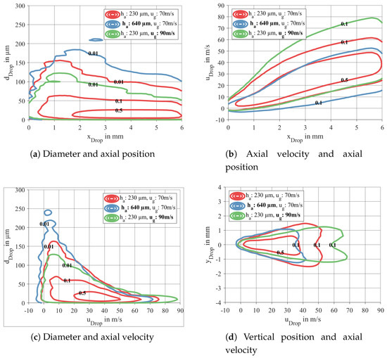
Figure 16.
Effect of gas velocity and prefilmer geometry on the interdependencies of the spray quantities for = 5 bar.
The change of the velocity vectors due to an increase of and is depicted in Figure 17a. Obviously, the former leads to higher axial velocities and the latter to lower ones compared to the baseline case. The lines of constant probability () scale in size and their shape is identical since all three cases are subject to the same breakup mechanism. Consequently, the droplet trajectories and the spray cones as depicted in Figure 17b are only slightly effected by and .
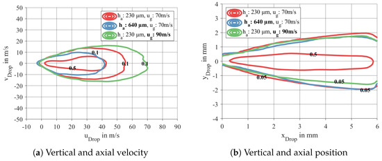
Figure 17.
Effect of gas velocity and prefilmer geometry on the interdependencies of the spray quantities for = 5 bar.
In summary, the qualitative characteristics, i.e., the shape of the joint probabilities of the spray quantities do not change with and . This is reasonable, as all simulations belong to the same regime of prefilming airblast atomization. However, and have a major effect on the shape of the distributions of and . A change in also effects . Regarding and , only minor effects of and can be observed.
5. Conclusions
Detailed simulations of a prefilming airblast atomizer using the Smoothed Particle Hydrodynamics (SPH) method have been presented. While the simulations are 2D, most of the breakup characteristics observed in experiments can be reproduced. Different effects of the film waves and the drag forces on the ligaments are discussed. Strong links between the ligament breakup and the resulting spray in terms of size, position and velocity of the droplets are demonstrated. The SPH simulations resemble quite well the effects observed by experiments. Hence, reliable spray characteristics close to the fuel nozzle and in particular at elevated pressure can be generated by the SPH method. This enables the usa of SPH data for the development of primary atomization models. Regarding the spray, significant interdependencies between droplet diameter, position and velocity are observed. The effects of gas velocity and trailing edge thickness on these interdependencies are outlined. In future work, these interdependencies will be further analysed and modelled using multivariate statistical methods.
Supplementary Materials
The following are available online at https://www.mdpi.com/1996-1073/12/14/2835/s1. Video S1: Breakup Sequence.
Author Contributions
Conceptualization, S.H., G.C., R.K.; data curation, S.H., S.B.; formal analysis, S.H.; funding acquisition, R.K., H.-J.B.; investigation, S.H., S.B., G.C., R.K.; methodology, S.H., S.B.; project administration, R.K.; resources, H.-J.B.; software, S.B., S.H.; supervision, R.K.; validation, S.B., G.C., S.H.; visualization, S.H.; writing—original draft preparation, S.H.; writing—review and editing, S.H., S.B., G.C., R.K.
Funding
This research was partially funded by the German aeronautical research program LuFo V within the project EmKoVal.
Acknowledgments
The numerical computations were performed on the high performance computing cluster ForHLR I at the Karlsruhe Institute of Technology. The cluster is funded by the Ministry of Science, Research and the Arts Baden Württemberg and the DFG (“Deutsche Forschungsgemeinschaft”). We acknowledge support by the KIT-Publication Fund of the Karlsruhe Institute of Technology.
Conflicts of Interest
The authors declare no conflict of interest.
Appendix A. Non Dimensional Quantities
The following non-dimensional quantities can be defined for prefilming airblast atomization:
Ratio of momentum fluxes:
The velocity of the liquid is set equal to the film velocity at the inlet: = m/s.
Weber number based on the height of the trailing edge :
Reynolds number based on the thickness of the turbulent boundary layer :
Weber number based on the thickness of the turbulent boundary layer :
Density ratio:
Non-dimensional trailing edge thickness:
As length scale, the thickness of the turbulence boundary layer at the end of the prefilmer can be applied. Following the definition of [38] leads to:
Please note that is set to 71 mm in the present study, which is similar to the length of the prefilmer in the experiment.
Appendix B. SMD-Correlation of Gepperth
Gepperth [31] derived a correlation for the SMD of the spray downstream from a prefilming airblast atomizer using a shadowgraphy technique. During the experimental study, the air pressure was increased up to 8 bar and the air velocity was varied from 20 to 80 m/s, leading to 350 experimentally investigated operating points including different trailing edge thicknesses.
References
- Lefebvre, A.H.; Ballal, D.R. Gas Turbine Combustion: Alternative Fuels and Emissions, 3rd ed.; CRC Press: Boca Raton, FL, USA, 2012. [Google Scholar]
- Gosman, A.D.; Ioannides, E. Aspects of Computer Simulation of Liquid-Fueled Combustors. J. Energy 1983, 7, 482–490. [Google Scholar] [CrossRef]
- Gallot-Lavallée, S.; Jones, W.; Marquis, A. Large Eddy Simulation of an ethanol spray flame under MILD combustion with the stochastic fields method. Proc. Combust. Inst. 2017, 36, 2577–2584. [Google Scholar] [CrossRef]
- Puggelli, S.; Paccati, S.; Bertini, D.; Mazzei, L.; Andreini, A.; Giusti, A. Multi-coupled numerical simulations of the DLR Generic Single Sector Combustor. In Proceedings of the Tenth Mediterranean Combustion Symposium, Naples, Italy, 17 September 2017. [Google Scholar]
- Comer, A.L.; Kipouros, T.; Cant, R.S. Multi-objective Numerical Investigation of a Generic Airblast Injector Design. J. Eng. Gas Turbines Power 2016, 138, 091501. [Google Scholar] [CrossRef]
- Keller, J.; Gebretsadik, M.; Habisreuther, P.; Turrini, F.; Zarzalis, N.; Trimis, D. Numerical and experimental investigation on droplet dynamics and dispersion of a jet engine injector. Int. J. Multiph. Flow 2015, 75, 144–162. [Google Scholar] [CrossRef]
- El-Asrag, H.A.; Iannetti, A.C.; Apte, S.V. Large eddy simulations for radiation-spray coupling for a lean direct injector combustor. Combust. Flame 2014, 161, 510–524. [Google Scholar] [CrossRef]
- Jones, W.; Marquis, A.; Vogiatzaki, K. Large-eddy simulation of spray combustion in a gas turbine combustor. Combust. Flame 2014, 161, 222–239. [Google Scholar] [CrossRef]
- Jaegle, F.; Senoner, J.M.; García, M.; Bismes, F.; Lecourt, R.; Cuenot, B.; Poinsot, T. Eulerian and Lagrangian spray simulations of an aeronautical multipoint injector. Proc. Combust. Inst. 2011, 33, 2099–2107. [Google Scholar] [CrossRef]
- Holz, S.; Chaussonnet, G.; Gepperth, S.; Koch, R.; Bauer, H.J. Comparison of the Primary Atomization Model PAMELA with Drop Size Distributions of an Industrial Prefilming Airblast Nozzle. In Proceedings of the 27th Annual Conference on Liquid Atomization and Spray Systems, Brighton, UK, 4–7 September 2016. [Google Scholar]
- Warncke, K.; Gepperth, S.; Sauer, B.; Sadiki, A.; Janicka, J.; Koch, R.; Bauer, H.J. Experimental and numerical investigation of the primary breakup of an airblasted liquid sheet. Int. J. Multiph. Flow 2017, 91, 208–224. [Google Scholar] [CrossRef]
- Volz, M.; Habisreuther, P.; Zarzalis, N. Correlation for the Sauter Mean Diameter of a Prefilmer Airblast Atomizer at Varying Operating Conditions. Chem. Ing. Tech. 2016. [Google Scholar] [CrossRef]
- Bilger, C.; Cant, S. Mechanisms of Atomization of a Liquid-Sheet: A Regime Classification. In Proceedings of the 27th Annual Conference on Liquid Atomization and Spray Systems, Brighton, UK, 4–7 September 2016. [Google Scholar]
- Braun, S.; Wieth, L.; Holz, S.; Dauch, T.F.; Keller, M.C.; Chaussonnet, G.; Gepperth, S.; Koch, R.; Bauer, H.J. Numerical prediction of air-assisted primary atomization using Smoothed Particle Hydrodynamics. Int. J. Multiph. Flow 2019, 114, 303–315. [Google Scholar] [CrossRef]
- Dauch, T.F.; Braun, S.; Wieth, L.; Chaussonnet, G.; Keller, M.C.; Koch, R.; Bauer, H.J. Computational Prediction of Primary Breakup in Fuel Spray Nozzles for Aero-Engine Combustors. In Proceedings of the 28th Conference on Liquid Atomization and Spray Systems, València, Spain, 6–8 September 2017. [Google Scholar] [CrossRef]
- Gingold, R.; Monaghan, J.J. Smoothed particle hydrodynamics: theory and application to non-spherical stars. Mon. Not. R. Astron. Soc. 1977, 181, 375–389. [Google Scholar] [CrossRef]
- Lucy, L.B. A numerical approach to the testing of the fission hypothesis. Astron. J. 1977, 82, 1013–1024. [Google Scholar] [CrossRef]
- Monaghan, J.J.; Kocharyan, A. SPH simulation of multi-phase flow. Comput. Phys. Commun. 1995, 87, 225–235. [Google Scholar] [CrossRef]
- Chaussonnet, G.; Braun, S.; Dauch, T.; Keller, M.; Sänger, A.; Jakobs, T.; Koch, R.; Kolb, T.; Bauer, H.J. Toward the development of a virtual spray test-rig using the Smoothed Particle Hydrodynamics method. Comput. Fluids 2019, 180, 68–81. [Google Scholar] [CrossRef]
- Hoefler, C.; Braun, S.; Koch, R.; Bauer, H.J. Modeling Spray Formation in Gas Turbines—A New Meshless Approach. J. Eng. Gas Turbines Power 2012, 135, 011503. [Google Scholar] [CrossRef]
- Wendland, H. Piecewise polynomial, positive definite and compactly supported radial functions of minimal degree. Adv. Comput. Math. 1995, 4, 389–396. [Google Scholar] [CrossRef]
- Wang, Z.B.; Chen, R.; Wang, H.; Liao, Q.; Zhu, X.; Li, S.Z. An overview of smoothed particle hydrodynamics for simulating multiphase flow. Appl. Math. Model. 2016, 40, 9625–9655. [Google Scholar] [CrossRef]
- Brackbill, J.; Kothe, D.; Zemach, C. A continuum method for modeling surface tension. J. Comput. Phys. 1992, 100, 335–354. [Google Scholar] [CrossRef]
- Adami, S.; Hu, X.; Adams, N. A new surface-tension formulation for multi-phase SPH using a reproducing divergence approximation. J. Comput. Phys. 2010, 229, 5011–5021. [Google Scholar] [CrossRef]
- Wieth, L.; Braun, S.; Koch, R.; Bauer, H.J. Modeling of liquid-wall interaction using the Smoothed Particle Hydrodynamics (SPH) method. In Proceedings of the 26th Annual Conference on Liquid Atomization and Spray Systems, Bremen, Germany, 8–10 September 2014. [Google Scholar]
- Braun, S.; Koch, R.; Bauer, H.J. Smoothed Particle Hydrodynamics for Numerical Predictions of Primary Atomization. In High Performance Computing in Science and Engineering’16; Springer Nature: Basingstoke, UK, 2016; pp. 321–336. [Google Scholar]
- Koch, R.; Braun, S.; Wieth, L.; Chaussonnet, G.; Dauch, T.; Bauer, H.J. Prediction of primary atomization using Smoothed Particle Hydrodynamics. Eur. J. Mech. B/Fluids 2017, 61, 271–278. [Google Scholar] [CrossRef]
- Dauch, T.; Braun, S.; Wieth, L.; Chaussonnet, G.; Keller, M.; Koch, R.; Bauer, H.-J. Computation of liquid fuel atomization and mixing by means of the SPH method: Application to a jet engine fuel nozzle. In Proceedings of the ASME Turbo Expo 2016: Turbine Technical Conference and Exposition GT2016, Seoul, Korea, 13–17 June 2016. [Google Scholar]
- Chaussonnet, G.; Gepperth, S.; Holz, S.; Koch, R.; Bauer, H.J. Influence of the ambient pressure on the liquid accumulation and on the primary spray in prefilming airblast atomization. arXiv 2019, arXiv:1906.04042. [Google Scholar]
- Gepperth, S.; Müller, A.; Koch, R.; Bauer, H.J. Ligament and droplet characteristics in prefilming airblast atomization. In Proceedings of the 12th Triennial International Annual Conference on Liquid Atomization and Spray Systems, Heidelberg, Germany, 2–6 September 2012. [Google Scholar]
- Gepperth, S. Experimentelle Untersuchung des Primärzerfalls an generischen luftgestützten Zerstäubern unter Hochdruckbedingungen. Ph.D. Thesis, Fakultät für Maschinenbau, Karlsruher Institut für Technologie, Karlsruher, Germany, 2018. [Google Scholar]
- Landahl, M.T.; Mollo-Christensen, E. Turbulence and Random Processes in Fluid Mechanics; Cambridge University Press: Cambridge, UK, 1992. [Google Scholar] [CrossRef]
- Pfaltz, J.L. Sequential Operations in Digital Picture Processing. J. ACM 1966, 13, 471–494. [Google Scholar] [CrossRef]
- Gepperth, S.; Koch, R.; Bauer, H.J. Analysis and comparison of primary droplet characteristics in the near field of a prefilming airblast atomizer. In Proceedings of the ASME Turbo Expo 2013: Turbine Technical Conference and Exposition, San Antonio, TX, USA, 3–7 June 2013. [Google Scholar]
- Holz, S.; Braun, S.; Chaussonnet, G.; Dauch, T.; Kaden, J.; Keller, M.; Schwitzke, C.; Koch, R.; Bauer, H.J. New Insights in the Primary Breakup Process of Prefilming Airblast Atomizers by SPH Predictions. In Proceedings of the 14th International Conference on Liquid Atomization and Spray Systems, Chicago, IL, USA, 22–26 July 2018. [Google Scholar]
- Braun, S.; Wieth, L.; Koch, R.; Bauer, H.J. Influence of Trailing Edge Height on Primary Atomization: Numerical Studies Applying the Smoothed Particle Hydrodynamics (SPH) Method. In Proceedings of the 13th Triennial International Conference on Liquid Atomization and Spray System, Tainan, Taiwan, 23–27 August 2015. [Google Scholar]
- Steinbach, A.; Dittmann, T.; Gerlinger, P.; Aigner, M.; Eggels, R. Soot predictions in an aircraft combustor at realistic operating conditions. In Proceedings of the ASME Turbo Expo 2018 Turbomachinery Technical Conference and Exposition GT2018, Oslo, Norway, 11–15 June 2018. [Google Scholar]
- White, F.M.; Corfield, I. Viscous Fluid Flow; McGraw-Hill: New York, NY, USA, 2006; Volume 3. [Google Scholar]


© 2019 by the authors. Licensee MDPI, Basel, Switzerland. This article is an open access article distributed under the terms and conditions of the Creative Commons Attribution (CC BY) license (http://creativecommons.org/licenses/by/4.0/).