Abstract
Recently, we proposed an approximate expression for the liquid–vapor saturation curves of pure fluids in a temperature–entropy diagram that requires the use of parameters related to the molar heat capacity along the vapor branch of the saturation curve. In the present work, we establish a connection between these parameters and the ideal-gas isobaric molar heat capacity. The resulting new approximation yields good results for most working fluids in Organic Rankine Cycles, improving the previous approximation for very dry fluids. The ideal-gas isobaric molar heat capacity can be obtained from most Thermophysical Properties databases for a very large number of substances for which the present approximation scheme can be applied.
1. Introduction
There is an increasing interest in the use of Organic Rankine Cycles (ORCs) as a suitable way of generating power from low-temperature heat sources such as geothermal, solar thermal, biomass, waste heat, and bottoming cycles. As is well known, a key aspect in the optimal implementation of an ORC for a given heat source is the choice of the working fluid. An appropriate working fluid selection should take into account several criteria such as thermo-economic efficiency, safety, environmental aspects, chemical stability, etc. [1,2,3,4,5,6].
One of the most relevant aspects in ORC working fluid selection is the analysis of the shape of the liquid–vapor saturation curve in a temperature–molar entropy (T-s) diagram because it has a direct influence both in the thermal efficiency and in the particular design of the cycle. Let us consider a simple, ideal ORC with an evaporation temperature and a condensation temperature , so that where is the critical temperature. In this simple ORC, the isentropic expansion that takes place in the turbine and starts from a saturated vapor state at can lead to three different situations depending on the shape of the saturation curve: (1) If the mean slope of the vapor branch of the T-s saturation curve between and is negative, the working fluid has a wet fluid behavior and the isentropic expansion process in the turbine gives rise to condensation, i.e., it ends in the two-phase region of the T-s diagram. This situation should be avoided (via superheating) since the mixture of vapor with liquid droplets could lead to damage of the turbine blades [7]. (2) If the mean slope is positive, the working fluid has a dry fluid behavior and the isentropic expansion leads to superheated vapor. This implies a reduction in the cycle efficiency which can only be partially remediated by resorting to a regenerator. (3) Finally, if the absolute value of the mean slope is very large, the working fluid behaves as an isentropic fluid so that the turbine isentropic expansion ends near the saturated vapor state at . In this case, neither regeneration nor superheating is required.
Fluids such as water, carbon dioxide or ammonia that always have a negative slope in the vapor branch of the T-s saturation curve () always behave as wet fluids and are usually termed as wet. On the other hand, fluids such as siloxanes or alkanes with a large number of carbons have a positive slope for most temperatures in the T-s saturation curve and are called dry fluids since they usually lead to a dry fluid behavior. Finally, fluids like the refrigerants RE143a, R11, or R116 present a wide range of temperatures for which the saturated vapor curve is almost vertical. These fluids are usually termed as isentropic, although isentropic behavior can also be obtained with a particular class of dry fluids [8,9,10]. To summarize, the slope of the vapor branch of the T-s saturation curve gives rise to a basic classification of working fluids into three categories: wet, dry, and isentropic. According to Liu et al. dry or isentropic fluids are preferred for ORC applications since they eliminate the problems related to condensation in the isentropic expansion [7].
Most studies on the shape of the T-s saturation boundary have focused in the analysis of the slope of the vapor branch and its relation with the molar heat capacity of the fluid. In a seminal work, Morrison [11] presented a study in the context of refrigeration cycles, concluding that negative slopes in the vapor branch do arise for fluids with large isochoric molar heat capacity and, consequently, for fluids with large, complex molecules. Liu et al. [7] derived an approximate expression of the (inverse) slope in terms of the isobaric molar heat capacity of the saturated vapor and the molar enthalpy of vaporization, and related the dry or wet character of the fluid to the sign of . Other authors have obtained results for different model equations of state, concluding that a key aspect in the shape of the T-s saturation curve is the ideal gas contribution to the molar heat capacity of the fluid [12,13,14,15].
Recently [16], we proposed a semiempirical method to obtain the T-s saturation curve by means of: (1) a modified rectilinear diameter law for the two branches of the saturated entropy; and (2) an appropriate expression for the entropy of vaporization . The method only requires the knowledge of three parameters: , the acentric factor , and the slope of the modified rectilinear diameter . Two approximations were considered for b. The simplest one requires the knowledge of the critical molar volume , which together with and can be obtained in any Thermophysical Properties database. The most accurate approximation requires the calculation of the slope at a certain temperature and therefore, the use of programs like RefProp [17] or CoolProp [18]. The goal of the present work is to study the relation between the modified rectilinear diameter law and the ideal gas molar heat capacity considered in earlier works [12,13,14,15]. More concretely, in this work, we propose a new approximation for b in terms of and the ideal-gas isobaric molar heat capacity at an appropriate reduced temperature. The new approximation has the same application range as the previous ones, with the advantage that it does not require the calculation of and yields better results for very dry fluids.
This paper is structured as follows. In Section 2, we outline the main features of the semiempirical method in [16]. In Section 3, we introduce the ideal gas contribution to the entropy and investigate its relevance in the dry or wet behavior of a working fluid. From the results of the preceding sections, a new approximation for the slope of the modified rectilinear diameter is proposed in Section 4, in terms of the ideal gas molar heat capacity of the fluid. In Section 5, we compare the results of the new approximation with previous ones. Finally, we conclude in Section 6 with a brief summary.
2. A Semiempirical Method for the - Saturation Curve
In [16], we proposed a semiempirical method to obtain approximate expressions for the liquid–vapor phase boundary in a temperature–entropy diagram. Here, we present the basic equations of the method that are employed in connection with the ideal gas molar heat capacity of the fluid. We find it convenient to work in reduced coordinates so that, without loss of generality, we consider a diagram where is the reduced temperature and is a dimensionless molar entropy, where is the molar critical entropy and R is the gas constant. In this context, the entropies of the gas and liquid branches of the phase boundary are denoted as and , respectively, and are functions of . Furthermore, with these definitions, for all fluids, one has .
To determine and , two relations are considered in the semiempirical method. The first one is the well-known relation between the dimensionless molar enthalpy of vaporization and the molar entropy of vaporization :
Several approximate expressions for are available in the literature [19]. For simplicity, we consider the following corresponding states version [20] of the Watson equation [21]:
where
is a function of the acentric factor of the fluid .
The second relation in the semiempirical method is based on the observation [16] that the line of constant quality q in the two-phase region of the diagram,
has an approximately linear behavior in the range for an appropriate value of q. The optimal value of q varies slightly with the fluid, with a mean value for the 121 fluids of the RefProp 9.1 program [17]. Therefore, one can write the following modified rectilinear diameter relation for the entropies of the saturated liquid and vapor [16]:
where is the slope of the modified rectilinear diameter. We note here that this linear relation is similar to the well known rectilinear diameter law of Cailletet and Mathias [22] for the saturation densities but, instead of using , one has to consider a different value of q for the entropy.
Equations (1) and (4) allow expressing the saturation entropies in terms of and :
that are exact relations valid for any value of the quality in the range . Substituting the approximations Equations (2) and (5) with , it is direct to obtain the approximate expressions
which are expected to yield good results for the entropies of the saturated vapor and liquid in the range . Equations (8) and (9) require the parameter b as an input. Differentiating Equation (8) with respect to one has
From this equation, two approximations were considered in [16] for b. The first one, referred to as approximation A1, is given by the following expression:
where is the reduced temperature at which the derivative attains its maximum value (see [16,23] for details). The values of and have been calculated in [23] for the 121 pure fluids of RefProp 9.1. From now on, all results obtained from this approximation are labeled with the subscript A1, i.e., we refer to , , , and .
To avoid the dependence of the parameter b on and , a further approximation A2 was presented in [16], in which was replaced by its mean value and a correlation in terms of the critical molar volume was used for . Approximation A1 is more accurate, but approximation A2 only depends on , , and that are easily accessible for several fluids.
3. The Ideal Gas Contribution to the Entropy
The dimensionless molar entropy of a fluid can be expressed as
where is the reduced volume, is a dimensionless residual entropy (that depends on the equation of state of the fluid), and is the ideal gas contribution to the entropy:
In Equation (13), the subscript 0 refers to an arbitrary reference state and is the dimensionless ideal gas isobaric heat capacity. Several approximate expressions for have been used in the literature. Common choices are polynomial expansions of the form
and the well-known Aly-Lee equation [24] used by the DIPPR database [25]
where the parameters ( in Equation (14)) are obtained by a fit to experimental data, and are, therefore, fluid-dependent. Furthermore, it is worth mentioning that, depending on the fluid, the RefProp 9.1 program [17] uses different approximate expressions for that provide an accurate fit to experimental data.
We find it convenient to split the ideal gas contribution to the entropy in two parts:
where
and
so that carries the temperature dependence of the dimensionless molar entropy due to , and is a function of the temperature and the molar volume. From Equations (12) and (16)–(18), one can write the following expressions for the entropies of the saturated vapor and liquid
where and are, respectively, the reduced volumes of the saturated vapor and liquid. The excess entropy , is a function of the reduced temperature and the reduced volume of the fluid. Equations (19) and (20) show that the entropies of the saturated liquid and vapor can be separated in two contributions. The first one, , is the same for the two saturated phases and only depends on through an integral of . The second contribution is different for each saturated phase and depends on the equation of state of the fluid.
The behavior of the ideal gas contribution defined in Equation (17) is shown in Figure 1 in a diagram for: (a) ammonia; (b) benzene; and (c) methyl palmitate. In this figure, one can see that the main source for the inclination of the saturation boundary is the ideal gas contribution . This implies that the dry or wet character of a fluid is mainly driven by the slope of . This fact was previously observed by Groniewsky and coworkers [14,15], but using the contribution to the molar entropy due to the isochoric molar heat capacity of the ideal gas instead of the isobaric one, .
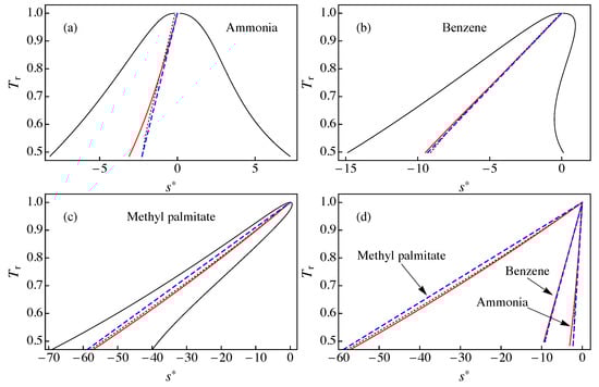
Figure 1.
- diagram for: (a) ammonia; (b) benzene; and (c) methyl palmitate. The solid red line corresponds to the ideal gas contribution to the entropy defined in Equation (17), the dotted black line is the constant quality entropy obtained from Equation (4) with , and the dashed blue line shows with b obtained from Equation (11) (approximation A1). The solid black line represents the liquid–vapor saturation boundary. (d) A comparison of the results for , , and presented in (a–c). All data were obtained using RefProp 9.1 [17].
We also show in Figure 1 the line of constant quality (with ) obtained from Equation (4) using RefProp 9.1 results [17] for and , and the result of approximation A1 for the modified rectilinear diameter relation in Equation (5) with the parameter given by Equation (11). To calculate , the following values were used [23] (see also Table A1): , , and for ammonia; , , and for benzene; and , , and for methyl palmitate. We obtained for ammonia, for benzene, and for methyl palmitate.
In Figure 1a, we consider ammonia as an example of wet fluid. As one can observe, in this case, the ideal gas contribution shows a noticeable deviation from both the line of constant quality obtained from RefProp 9.1 and the approximate (straight line) result . The best agreement for ammonia was obtained for . Much better agreement was obtained for benzene (Figure 1b), especially in the range 0.7 < < 0.99. The case of methyl palmitate presented in Figure 1c shows a good agreement between and , with larger deviations with . We note that methyl palmitate is a “very dry” fluid, with a large value of and approximation A1 is known to give large deviations for these fluids [16]. In Figure 1d, we plot the results for , , and in the same scale, showing that the main discrepancies take place between and for methyl palmitate.
From the results presented in Figure 1, which are also valid for the remaining fluids of RefProp 9.1 (not shown), we can conclude that the ideal gas contribution is close to the line of constant quality with but some differences do arise, especially for < 0.7. Therefore, it is not advisable to replace with in Equations (6) and (7) in order to obtain a new approximation for the entropy of the saturation boundary. As shown in the next section, it is more convenient to consider the approximate expressions of Equations (8) and (9) but using information from instead of Equation (11).
4. A New Approximation for the - Saturation Curve
Differentiating Equation (19) with respect to , we obtain the following expression for the slope of the entropy of the saturated vapor
where
We note that, as pointed out by Garrido et al. [12], according to Equation (21), a fluid behaves as dry for reduced temperatures such that
A rigorous approach for obtaining from an explicit equation of state (Eos) model has been developed by Garrido et al. [12]. This implies that should be correlated with the acentric factor of the fluid. In Figure 2, we plot vs. for the 121 fluids of RefProp 9.1 [17] at a reduced temperature , which is taken as reference. Instead of considering a given Eos model, the values of were obtained from Equation (21) and RefProp 9.1 data for and . As one can observe, there is a rather good correlation between and . A quadratic fit excluding two oddball fluids (ethanol and methanol, black dots in Figure 2) yields
with a coefficient of determination .
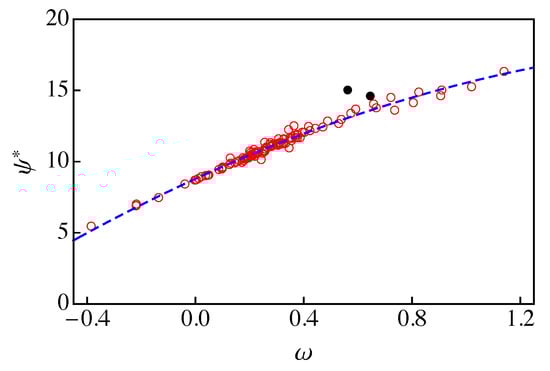
Figure 2.
vs. for the 121 fluids of RefProp 9.1 [17] at a reduced temperature . The dashed blue line is the result of a quadratic fit to the data (red circles) excluding ethanol and methanol (solid black circles).
Equating Equations (10) and (21) and taking as reference the reduced temperature , we obtain
where the label A3 has been chosen to compare with approximations A1 and A2 in [16], and, using Equations (3) and (24),
Finally, inserting Equation (25) into Equations (8) and (9), we obtain
which are the results of our new approximation A3 for the entropies of the saturated vapor and liquid. Taking into account that the new approximation is also based in the modified rectilinear diameter relation in Equation (5), we expect that the results of A3 should apply in the range . We would like to recall here that Equations (27) and (28) only require the knowledge of the acentric factor of the fluid, its critical temperature, and the ideal gas molar isobaric heat capacity at a reduced temperature . These parameters are easily accessible for a large amount of fluids using well known databases such as DIPPR [25].
5. Results
Figure 3 compares the results of RefProp 9.1 with those of approximations A1 and A3 for the liquid–vapor saturation boundary in a diagram for: (a) ammonia; (b) benzene; (c) methyl palmitate;and (d) D6. In the case of ammonia, approximation A3 gave better agreement with RefProp 9.1 than A1 for the saturated vapor branch, whereas we obtained the opposite behavior for the saturated liquid branch. This can be ascribed to the fact that the slope of the modified rectilinear diameter is slightly larger for A3 (, obtained from Equation (25) with ) than for A1 (). Figure 3b shows that A1 and A3 yield similar results for the saturation entropies of benzene, with excellent agreement with RefProp 9.1 results except for for . In this case, the slope is very similar to (obtained from ). In Figure 3c, the approximation A3 gives a better agreement with RefProp 9.1 than A1. This indicates that the slope (obtained from ) yields better results than that of approximation A1 (). Finally, Figure 3d shows that A3 yields much better agreement with RefProp 9.1 than A1. We note that D6 gives rise to the maximum deviation between A1 and RefProp 9.1, as we shown below. This is clearly due to the fact that the slope for D6 is much larger than .
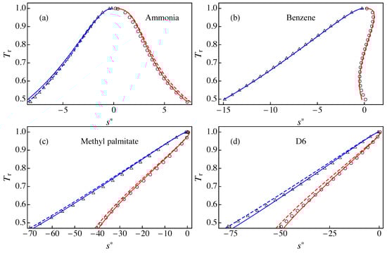
Figure 3.
Liquid–vapor saturation boundary in a - diagram for: (a) ammonia; (b) benzene; (c) methyl palmitate; and (d) D6. The solid lines correspond to the results of approximation A3 for the entropies of the saturated vapor (solid red line) and the saturated liquid (solid blue line). The dashed lines correspond to the results of approximation A1 for the entropies of the saturated vapor (dashed red line) and the saturated liquid (dashed blue line). The symbols are RefProp 9.1 results for (circles) and (triangles).
The only difference between approximations A1 and A3 comes from the value of the parameter b that is calculated from Equation (11) in the case A1 and from Equation (25) for A3. In Figure 4, we present a plot of vs. for the 121 fluids of RefProp 9.1 [17], which are also listed in Table A1. In all cases, we obtained negative values of b in the range −130 < b < −1 (notice that the modified rectilinear diameter relation is given by and thus the slope of the straight line, , is always positive). Overall, the agreement between both approaches is very good except for very dry fluids (with large values of ) where approximation A3 yields results for slightly smaller than those of approximation A1, as one can see in Figure 4a. Wet fluids are those for which and thus they present smaller values of . As shown in Figure 4b, the agreement between the results of A1 and A3 for wet fluids is still good but presents more spread. The transition from dry to wet fluids occurs for but it is not sharp, mainly due to the effect of the acentric factor in Equation (11).
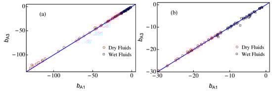
Figure 4.
The parameter vs. . The symbols represent the values of and obtained from Equations (25) and (11), respectively, using RefProp 9.1 data [17]. The solid blue line corresponds to the identity . Dry fluids () are plotted with red circles and wet fluids () correspond to black squares. (b) A zoom of (a). The data for and are listed in Table A1.
To provide a quantitative measurement of the performance of approximations A1 and A3, we consider the following expression for the percent relative deviation of approximation Ai (), which was introduced in [16]:
where and are RefProp 9.1 results. We obtained and for ammonia, and for benzene, and and for methyl palmitate.
Figure 5 compares the percent relative deviations of A1 and A3 for the 121 fluids of RefProp 9.1. To relate the performance of A1 and A3 to the dry or wet character of the fluid, the percent relative deviations are plotted as a function of the parameter . We note that, for the sake of clarity, the results are plotted with lines instead of symbols. As one can observe in Figure 5 (see also Table A1) the new approximation A3 fares better than A1 for fluids with , i.e., for very dry fluids. For the remaining fluids, both approximations yield similar results, in most cases with relative deviations less than (below the dotted line in Figure 5). More concretely, in the case of the new approximation A3, we obtained an average percent relative deviation for all fluids of Table A1, with a maximum percent relative deviation for methyl stearate (the only fluid with ). In the case of A1, one has [16] and for D6, with nine fluids of a total of 121 with . The reason for obtaining can be clearly ascribed to the poorer behavior of A1 for very dry fluids. We note, however, that, in the two approximate treatments, 96 fluids have relative deviations less than . Among the wet fluids (), the largest relative deviations were obtained for helium ( and ) and R40 ( and ). Finally, we would like to note that, even with large deviations, e.g. for D6, one can obtain fairly good results, as shown in Figure 3d.
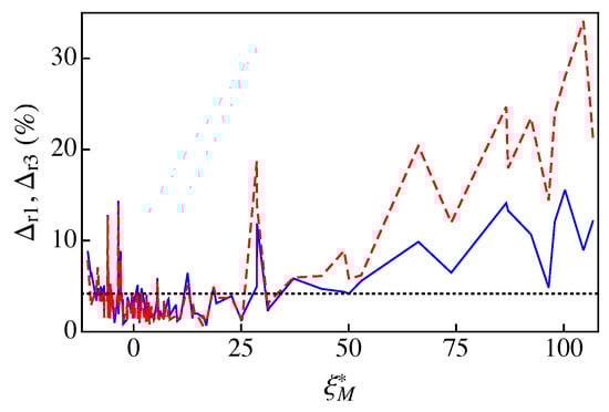
Figure 5.
The percent relative deviations and vs. . For clarity, the deviations are plotted with lines: the dashed red line corresponds to and the solid blue line represents . The dotted line indicates a deviation level of . The data for , , and are listed in Table A1.
6. Summary
In a previous work [16], a semiempirical method was developed for obtaining the liquid–vapor boundary of a fluid in a diagram. The method assumes that, for a certain value of the quality , the line of constant in the diagram () is very close to the straight line , i.e., one has a modified rectilinear diameter relation for the saturation entropies. From this assumption, the semiempirical method only requires two ingredients: an appropriate expression for the enthalpy of vaporization and an approximate estimation of the parameter b. In what refers to the enthalpy of vaporization, perhaps the simplest choice is the extended corresponding states version [20] of the Watson equation [21] considered in [16] and in the present work. Two approximations, A1 and A2, where developed for b in [16]. The more accurate is approximation A1 with given by Equation (11) and therefore depending on the acentric factor , the parameter , and the reduced temperature . The main drawback of A1 is that, while is available for most fluids, the other two parameters must be calculated for each fluid. Approximation A2 is less accurate but it has the advantage that, in addition to , it only requires the critical molar volume that can be accessed in most databases.
In the present work, we developed a new approximation A3 where the parameter is given by Equation (25) and only depends on and on the ideal-gas isobaric molar heat capacity of the fluid at a reduced temperature . We want to recall that excellent approximations for are available for a large variety of fluids in most Thermophysical Properties databases. The new approximation has the virtues of approximations A1 and A2 without their problems: it has an accuracy similar to or even better than that of A1 and only needs the value of easily accessible parameters.
To conclude we would like to comment that the present work has also served to clarify the role played by the ideal-gas isobaric molar heat capacity in the shape of the liquid–vapor saturation boundary in a temperature–entropy diagram, in agreement with the results of other authors [11,12,13,14,15].
Author Contributions
Conceptualization, J.A.W. and S.V.; Formal analysis, J.A.W. and S.V.; and Writing—Original draft, J.A.W. and S.V.
Funding
This research was funded by Junta de Castilla y León of Spain grant number SA017P17.
Conflicts of Interest
The authors declare no conflict of interest.
Nomenclature
| Slope of the modified rectilinear diameter | |
| Percent relative deviation | |
| Molar enthalpy of vaporization, J/mol | |
| Molar volume, m/kmol | |
| Isobaric molar heat capacity, J/(mol K) | |
| p | Pressure, MPa |
| q | Quality |
| R | Gas constant, 8.314472 J/(molK) |
| s | Molar entropy, J/(molK) |
| T | Temperature, K |
| Greek letters | |
| Acentric factor | |
| Inverse of the slope of the saturated vapor curve, J/(molK) | |
| Superscripts | |
| ∗ | Dimensionless |
| ex | Excess |
| ig | Ideal gas |
| r | Residual |
| Subscripts | |
| A1, A2, A3 | Approximations used in this work |
| c | Critical |
| con | Condensation |
| ev | Evaporation |
| g | Saturated vapor |
| l | Saturated liquid |
| M | Point for which presents a maximum |
| r | Reduced |
| Acronyms | |
| ORC | Organic Rankine cycle |
Appendix A

Table A1.
Critical temperature , acentric factor , maximum slope of the entropy of the saturated vapor , reduced temperature , ideal gas molar isobaric heat capacity , parameters and , and percent relative deviations and . The data were obtained from RefProp 9.1 [17]. The fluids are listed in increasing value of .
| Fluid | (K) | ||||||||
|---|---|---|---|---|---|---|---|---|---|
| methanol | 513.38 | 0.5625 | −10.6364 | 0.7874 | 6.3594 | −7.0892 | −9.1848 | 7.74 | 8.78 |
| heavy water | 643.85 | 0.364 | −9.877 | 0.8071 | 4.5129 | −4.7427 | −5.7266 | 2.86 | 6.06 |
| water | 647.1 | 0.3443 | −9.846 | 0.8018 | 4.2676 | −4.534 | −5.3207 | 2.96 | 6.51 |
| ammonia | 405.4 | 0.256 | −8.6109 | 0.8162 | 4.3795 | −4.4225 | −5.0275 | 4.82 | 3.42 |
| hydrogen chloride | 324.55 | 0.1288 | −8.3196 | 0.8228 | 3.5036 | −2.9154 | −3.4131 | 7.06 | 4.78 |
| R41 | 317.28 | 0.2004 | −7.9926 | 0.8146 | 4.2702 | −4.2672 | −4.6467 | 4.02 | 4.02 |
| carbon dioxide | 304.13 | 0.2239 | −7.9381 | 0.8219 | 4.1683 | −4.6244 | −4.6224 | 4.71 | 4.72 |
| R32 | 351.26 | 0.2769 | −7.7684 | 0.8198 | 5.0411 | −5.5457 | −5.9418 | 3.34 | 3.34 |
| xenon | 289.73 | 0.0036 | −7.6918 | 0.8142 | 2.5 | −1.8437 | −1.7513 | 3.95 | 4.69 |
| krypton | 209.48 | −0.0009 | −7.6578 | 0.8124 | 2.5 | −1.8225 | −1.738 | 4.31 | 4.99 |
| argon | 150.69 | −0.0022 | −7.6561 | 0.8117 | 2.5 | −1.8092 | −1.7342 | 2.99 | 3.6 |
| neon | 44.49 | −0.0387 | −7.3103 | 0.8012 | 2.5 | −1.7047 | −1.6313 | 4.27 | 4.81 |
| sulfur dioxide | 430.64 | 0.2557 | −7.2518 | 0.8202 | 5.0139 | −5.7622 | −5.8093 | 3.64 | 3.36 |
| nitrous oxide | 309.52 | 0.162 | −7.0185 | 0.8224 | 4.3649 | −4.6784 | −4.6055 | 4.23 | 4.71 |
| R23 | 299.29 | 0.263 | −6.8638 | 0.8205 | 5.4574 | −6.2521 | −6.3906 | 3.13 | 2.54 |
| carbon monoxide | 132.86 | 0.0497 | −6.8622 | 0.8091 | 3.5003 | −3.328 | −3.1301 | 3.61 | 5.08 |
| fluorine | 144.41 | 0.0449 | −6.8234 | 0.8118 | 3.5034 | −3.2888 | −3.1183 | 1.54 | 1.93 |
| nitrogen | 126.19 | 0.0372 | −6.8113 | 0.806 | 3.5004 | −3.2219 | −3.0899 | 2.61 | 3.62 |
| hydrogen sulfide | 373.1 | 0.1005 | −6.8028 | 0.8072 | 4.1079 | −4.1004 | −4.0548 | 3.59 | 3.91 |
| oxygen | 154.58 | 0.0222 | −6.72 | 0.8054 | 3.5014 | −3.1095 | −3.044 | 3.77 | 4.28 |
| ethylene | 282.35 | 0.0866 | −6.1541 | 0.8156 | 4.4571 | −4.518 | −4.4365 | 3.39 | 3.97 |
| deuterium | 38.34 | −0.136 | −6.0597 | 0.7992 | 2.5576 | −1.638 | −1.4702 | 3.7 | 4.24 |
| R40 | 416.3 | 0.243 | −6.0057 | 0.8311 | 5.2349 | −6.8109 | −6.0242 | 12.65 | 12.83 |
| methane | 190.56 | 0.0114 | −5.9212 | 0.7978 | 4.0063 | −3.8044 | −3.6343 | 1.57 | 2.11 |
| nitrogen trifluoride | 234.0 | 0.126 | −5.8855 | 0.8261 | 5.0065 | −5.3046 | −5.2579 | 6.46 | 6.78 |
| R14 | 227.51 | 0.1785 | −5.7507 | 0.8153 | 5.4035 | −6.1996 | −5.9544 | 2.73 | 4.29 |
| orthohydrogen | 33.22 | −0.218 | −5.5374 | 0.7814 | 2.5 | −1.1452 | −1.2508 | 4.27 | 4.75 |
| carbonyl sulfide | 378.77 | 0.0978 | −5.4797 | 0.8131 | 5.0426 | −5.3573 | −5.1989 | 1.53 | 2.64 |
| ethanol | 514.71 | 0.646 | −5.4382 | 0.8407 | 10.0811 | −13.1771 | −14.3512 | 1.56 | 4.68 |
| parahydrogen | 32.94 | −0.219 | −5.4225 | 0.7856 | 2.5 | −1.2215 | −1.2493 | 4.84 | 5.02 |
| hydrogen | 33.15 | −0.219 | −5.3996 | 0.7873 | 2.5 | −1.2346 | −1.2493 | 4.94 | 5.04 |
| ethane | 305.32 | 0.0995 | −4.838 | 0.8145 | 5.6208 | −6.0169 | −5.919 | 2.68 | 3.37 |
| R22 | 369.3 | 0.2208 | −4.8229 | 0.819 | 6.768 | −7.7051 | −7.8182 | 3.47 | 2.77 |
| R161 | 375.25 | 0.216 | −4.4255 | 0.8205 | 7.2552 | −8.0304 | −8.3988 | 2.05 | 0.98 |
| propyne | 402.38 | 0.204 | −3.5995 | 0.7971 | 7.7056 | −8.824 | −8.9033 | 4.22 | 3.92 |
| helium | 5.2 | −0.385 | −3.5483 | 0.7489 | 2.5 | −1.0479 | −1.0829 | 13.86 | 14.38 |
| R152a | 386.41 | 0.2752 | −3.4813 | 0.8223 | 8.3897 | −9.8009 | −10.0678 | 2.6 | 1.94 |
| R13 | 302.0 | 0.1723 | −3.3923 | 0.8226 | 7.1846 | −8.4474 | −8.1281 | 2.73 | 4.78 |
| cyclopropane | 398.3 | 0.1305 | −2.9929 | 0.8469 | 7.3234 | −8.2874 | −8.1353 | 7.88 | 8.84 |
| R21 | 451.48 | 0.2061 | −2.9492 | 0.818 | 8.1052 | −9.3764 | −9.4055 | 4.12 | 3.94 |
| propylene | 364.21 | 0.146 | −2.7352 | 0.8214 | 7.6869 | −8.7418 | −8.6436 | 3.39 | 4.04 |
| R143a | 345.86 | 0.2615 | −2.4733 | 0.8183 | 9.0101 | −10.6289 | −10.7696 | 2.09 | 1.83 |
| DME | 400.38 | 0.196 | −2.4475 | 0.8198 | 8.3359 | −9.7307 | −9.6474 | 3.03 | 3.56 |
| trifluoroiodomethane | 396.44 | 0.176 | −2.4241 | 0.7992 | 8.3047 | −9.5876 | −9.526 | 1.1 | 0.85 |
| R134a | 374.21 | 0.3268 | −1.5632 | 0.8172 | 10.3353 | −12.4667 | −12.7222 | 2.73 | 1.32 |
| R12 | 385.12 | 0.1795 | −1.508 | 0.8043 | 8.9565 | −10.516 | −10.345 | 1.23 | 2.2 |
| propane | 369.89 | 0.1521 | −1.3906 | 0.8214 | 8.8547 | −10.1711 | −10.1092 | 3.39 | 3.8 |
| R125 | 339.17 | 0.3052 | −0.5398 | 0.8089 | 10.8094 | −13.2288 | −13.1997 | 2.0 | 2.16 |
| acetone | 508.1 | 0.3071 | −0.3538 | 0.8173 | 11.3098 | −13.3968 | −13.8269 | 4.12 | 4.14 |
| RE143a | 377.92 | 0.289 | −0.1089 | 0.818 | 11.1559 | −13.3826 | −13.5488 | 1.71 | 1.47 |
| sulfur hexafluoride | 318.72 | 0.21 | −0.0175 | 0.8201 | 10.4336 | −12.3555 | −12.2969 | 3.52 | 3.85 |
| R142b | 410.26 | 0.2321 | 0.1386 | 0.8155 | 10.7276 | −12.8389 | −12.7565 | 2.49 | 2.99 |
| R11 | 471.11 | 0.1888 | 0.234 | 0.7864 | 10.4086 | −12.5436 | −12.1762 | 1.53 | 3.64 |
| R116 | 293.03 | 0.2566 | 0.4458 | 0.8128 | 11.087 | −13.5038 | −13.3111 | 2.89 | 4.02 |
| cis-butene | 435.75 | 0.202 | 0.9697 | 0.8248 | 11.1318 | −13.219 | −13.1247 | 4.54 | 5.13 |
| R1234ze | 382.51 | 0.313 | 1.0989 | 0.8034 | 12.2336 | −15.0186 | −14.9966 | 1.25 | 1.38 |
| 1-butene | 419.29 | 0.192 | 1.3717 | 0.823 | 11.331 | −13.4852 | −13.3283 | 3.11 | 4.1 |
| R1234yf | 367.85 | 0.276 | 1.3815 | 0.8076 | 12.1995 | −14.7444 | −14.7751 | 1.1 | 0.97 |
| R124 | 395.42 | 0.2881 | 1.5614 | 0.8091 | 12.4188 | −15.086 | −15.1036 | 2.17 | 2.07 |
| trans-butene | 428.61 | 0.21 | 1.6935 | 0.8185 | 11.7485 | −14.0718 | −13.9202 | 2.07 | 2.9 |
| isobutene | 418.09 | 0.193 | 1.8248 | 0.8193 | 11.7778 | −13.9628 | −13.8841 | 4.27 | 4.77 |
| R141b | 477.5 | 0.2195 | 2.3839 | 0.8112 | 12.3076 | −14.9281 | −14.6517 | 1.87 | 3.55 |
| R115 | 353.1 | 0.248 | 2.9004 | 0.8079 | 12.9368 | −15.8656 | −15.5554 | 1.01 | 1.9 |
| isobutane | 407.81 | 0.184 | 3.044 | 0.8223 | 12.6842 | −15.0477 | −14.9656 | 3.54 | 4.07 |
| R1233zd | 438.75 | 0.305 | 3.0552 | 0.7975 | 13.715 | −16.9118 | −16.786 | 1.27 | 1.43 |
| R123 | 456.83 | 0.2819 | 3.4213 | 0.7994 | 13.8353 | −16.9311 | −16.8226 | 1.04 | 1.31 |
| butane | 425.12 | 0.201 | 3.5432 | 0.8181 | 13.2787 | −15.7971 | −15.7709 | 3.05 | 3.21 |
| R1216 | 358.9 | 0.333 | 3.6838 | 0.8095 | 14.2629 | −17.844 | −17.6026 | 0.8 | 1.36 |
| R245fa | 427.16 | 0.3776 | 4.1683 | 0.8193 | 15.2535 | −18.9125 | −19.0593 | 2.73 | 1.96 |
| R236fa | 398.07 | 0.377 | 4.6989 | 0.7995 | 15.7142 | −19.5696 | −19.6248 | 1.28 | 1.28 |
| R114 | 418.83 | 0.2523 | 5.4626 | 0.7781 | 15.1045 | −18.7798 | −18.2512 | 1.94 | 3.41 |
| cyclopentane | 511.72 | 0.201 | 5.524 | 0.8268 | 14.8424 | −17.7562 | −17.7013 | 5.52 | 5.87 |
| R236ea | 412.44 | 0.369 | 5.7807 | 0.7922 | 16.5039 | −20.6118 | −20.5568 | 1.51 | 1.44 |
| R245ca | 447.57 | 0.355 | 5.9462 | 0.8074 | 16.4625 | −20.4352 | −20.4318 | 1.41 | 1.41 |
| R227ea | 374.9 | 0.357 | 6.0234 | 0.8071 | 16.5119 | −20.5427 | −20.5033 | 1.48 | 1.68 |
| benzene | 562.02 | 0.211 | 6.1558 | 0.8252 | 15.4544 | −18.5302 | −18.4997 | 2.11 | 2.28 |
| RE245cb2 | 406.81 | 0.354 | 7.0324 | 0.796 | 17.3379 | −21.6067 | −21.5073 | 1.39 | 1.36 |
| DEE | 466.7 | 0.281 | 7.039 | 0.8045 | 16.8075 | −20.4947 | −20.4877 | 3.34 | 3.38 |
| R218 | 345.02 | 0.3172 | 7.2705 | 0.8054 | 17.1169 | −21.2347 | −21.0463 | 1.59 | 2.63 |
| DMC | 557.0 | 0.346 | 7.3867 | 0.8129 | 16.9462 | −21.7114 | −20.982 | 2.91 | 2.14 |
| R113 | 487.21 | 0.2525 | 7.4017 | 0.7761 | 16.6127 | −20.7474 | −20.1141 | 2.43 | 2.28 |
| RE245fa2 | 444.88 | 0.387 | 7.9754 | 0.7977 | 18.1268 | −23.0079 | −22.6575 | 1.67 | 3.46 |
| neopentane | 433.74 | 0.1961 | 8.1324 | 0.8216 | 16.828 | −20.3068 | −20.1319 | 2.49 | 3.58 |
| isopentane | 460.35 | 0.2274 | 8.3612 | 0.8179 | 17.3273 | −20.9858 | −20.8834 | 1.81 | 2.43 |
| pentane | 469.7 | 0.251 | 8.4366 | 0.816 | 17.5954 | −21.4005 | −21.3204 | 1.33 | 1.81 |
| RC318 | 388.38 | 0.3553 | 9.8443 | 0.7961 | 19.431 | −24.4359 | −24.0982 | 1.76 | 2.96 |
| R365mfc | 460.0 | 0.377 | 10.1649 | 0.8151 | 19.9073 | −24.9196 | −24.8015 | 1.28 | 1.17 |
| toluene | 591.75 | 0.2657 | 10.8934 | 0.8121 | 19.8028 | −24.0839 | −24.1134 | 1.61 | 1.49 |
| cyclohexane | 553.6 | 0.2096 | 12.5657 | 0.8378 | 20.4864 | −24.9198 | −24.706 | 5.14 | 6.45 |
| hexane | 507.82 | 0.299 | 13.6814 | 0.8127 | 22.3454 | −27.3396 | −27.4114 | 1.87 | 1.46 |
| isohexane | 497.7 | 0.2797 | 13.7711 | 0.8125 | 22.2099 | −27.1569 | −27.1511 | 3.02 | 3.05 |
| RE347mcc | 437.7 | 0.403 | 14.2038 | 0.7903 | 23.5211 | −29.5492 | −29.405 | 2.02 | 1.97 |
| perfluorobutane | 386.33 | 0.371 | 14.8856 | 0.7876 | 23.6981 | −29.8004 | −29.4493 | 1.76 | 2.0 |
| m-xylene | 616.89 | 0.326 | 16.0966 | 0.8077 | 24.2987 | −30.1694 | −29.9569 | 0.7 | 1.58 |
| p-xylene | 616.17 | 0.324 | 16.0973 | 0.8127 | 24.3608 | −30.11 | −30.0235 | 1.82 | 1.82 |
| ethylbenzene | 617.12 | 0.305 | 16.926 | 0.8164 | 24.8511 | −30.6508 | −30.5343 | 1.03 | 0.68 |
| o-xylene | 630.26 | 0.312 | 17.4037 | 0.8105 | 25.3699 | −31.2593 | −31.2093 | 2.15 | 2.2 |
| methylcyclohexane | 572.2 | 0.234 | 18.5937 | 0.8222 | 25.7539 | −31.2969 | −31.316 | 4.93 | 4.82 |
| heptane | 540.13 | 0.349 | 19.2387 | 0.8059 | 27.2864 | −33.6527 | −33.7634 | 3.71 | 3.11 |
| perfluoropentane | 420.56 | 0.423 | 22.8082 | 0.7793 | 30.5375 | −38.5956 | −38.1795 | 3.7 | 3.92 |
| octane | 569.32 | 0.395 | 25.1117 | 0.8011 | 32.3926 | −40.2261 | −40.3133 | 1.37 | 1.19 |
| isooctane | 544.0 | 0.303 | 25.2627 | 0.8145 | 31.6407 | −38.968 | −38.9066 | 1.38 | 1.72 |
| novec649 | 441.81 | 0.471 | 28.6415 | 0.7003 | 34.7076 | −47.1405 | −43.6078 | 18.68 | 4.96 |
| MM | 518.7 | 0.418 | 28.6999 | 0.7645 | 35.4931 | −44.6629 | −44.2692 | 13.84 | 11.87 |
| nonane | 594.55 | 0.4433 | 31.1834 | 0.7963 | 37.5659 | −47.0458 | −46.9732 | 2.59 | 2.29 |
| propylcyclohhexane | 630.8 | 0.326 | 31.4514 | 0.8077 | 37.0298 | −45.5243 | −45.6744 | 3.26 | 2.55 |
| decane | 617.7 | 0.4884 | 37.192 | 0.7864 | 42.8909 | −53.8373 | −53.8158 | 5.94 | 5.84 |
| undecane | 638.8 | 0.539 | 43.7309 | 0.7863 | 48.299 | −61.1241 | −60.8093 | 6.12 | 4.7 |
| MDM | 564.09 | 0.529 | 48.9411 | 0.7539 | 51.8895 | −66.8028 | −65.1781 | 8.89 | 4.38 |
| dodecane | 658.1 | 0.574 | 50.0562 | 0.7743 | 53.7356 | −68.1724 | −67.75 | 5.8 | 4.17 |
| D4 | 586.49 | 0.592 | 52.9243 | 0.7727 | 56.3406 | −71.3409 | −71.0868 | 6.19 | 5.58 |
| MD2M | 599.4 | 0.668 | 66.2116 | 0.7353 | 66.5042 | −86.7477 | −84.1675 | 20.4 | 9.87 |
| D5 | 619.23 | 0.658 | 73.8466 | 0.7473 | 73.2238 | −93.8744 | −92.391 | 11.98 | 6.48 |
| methyl palmitate | 755.0 | 0.91 | 86.6279 | 0.7388 | 84.2017 | −110.949 | −107.9614 | 24.68 | 14.12 |
| methyl linolenate | 772.0 | 1.14 | 87.0511 | 0.7625 | 86.3193 | −114.2828 | −112.7746 | 17.94 | 13.3 |
| MD3M | 628.36 | 0.722 | 92.3726 | 0.7165 | 87.7973 | −114.4347 | −110.8565 | 23.44 | 10.69 |
| methyl linoleate | 799.0 | 0.805 | 96.4907 | 0.7361 | 91.2891 | −119.2024 | −115.8209 | 14.41 | 4.83 |
| methyl oleate | 782.0 | 0.906 | 97.9157 | 0.7395 | 92.9609 | −122.1459 | −118.7401 | 24.02 | 12.09 |
| methyl stearate | 775.0 | 1.02 | 100.2849 | 0.7366 | 95.3592 | −126.492 | −122.7452 | 27.94 | 15.56 |
| D6 | 645.78 | 0.736 | 104.5704 | 0.6897 | 95.7557 | −128.0031 | −120.7889 | 34.1 | 8.95 |
| MD4M | 653.2 | 0.825 | 106.7797 | 0.7384 | 100.342 | −129.7364 | −127.1614 | 21.34 | 12.13 |
References
- Saleh, B.; Koglbauer, G.; Wendland, M.; Fischer, J. Working fluids for low-temperature organic Rankine cycles. Energy 2007, 32, 1210–1221. [Google Scholar] [CrossRef]
- Quoilin, S.; Declaye, S.; Tchanche, B.F.; Lemort, V. Thermo-economic optimization of waste heat recovery Organic Rankine Cycles. Appl. Therm. Eng. 2011, 31, 2885–2893. [Google Scholar] [CrossRef]
- Wang, E.; Zhang, H.; Fan, B.; Ouyang, M.; Zhao, Y.; Mu, Q. Study of working fluid selection of organic Rankine cycle (ORC) for engine waste heat recovery. Energy 2011, 36, 3406–3418. [Google Scholar] [CrossRef]
- SprouseIII, C.; Depcik, C. Review of organic Rankine cycles for internal combustion engine exhaust waste heat recovery. Appl. Therm. Eng. 2013, 51, 711–722. [Google Scholar] [CrossRef]
- Bao, J.; Zhao, L. A review of working fluid and expander selections for organic Rankine cycle. Renew. Sust. Energ. Rev. 2013, 24, 325–342. [Google Scholar] [CrossRef]
- Hærvig, J.; Sørensen, K.; Condra, T. Guidelines for optimal selection of working fluid for an organic Rankine cycle in relation to waste heat recovery. Energy 2016, 96, 592–602. [Google Scholar] [CrossRef]
- Liu, B.T.; Chien, K.H.; Wang, C.C. Effect of working fluids on organic Rankine cycle for waste heat recovery. Energy 2004, 29, 1207–1217. [Google Scholar] [CrossRef]
- Györke, G.; Deiters, U.K.; Groniewsky, A.; Lassu, I.; Imre, A.R. Novel classification of pure working fluids for Organic Rankine Cycle. Energy 2018, 145, 288–300. [Google Scholar] [CrossRef]
- Györke, G.; Groniewsky, A.; Imre, A.R. A Simple Method of Finding New Dry and Isentropic Working Fluids for Organic Rankine Cycle. Energies 2019, 12, 480. [Google Scholar] [CrossRef]
- Imre, A.R.; Kustán, R.; Groniewsky, A. Thermodynamic Selection of the Optimal Working Fluid for Organic Rankine Cycles. Energies 2019, 12, 2028. [Google Scholar] [CrossRef]
- Morrison, G. The shape of the temperature-entropy saturation boundary. Int. J. Refrig 1994, 17, 494–504. [Google Scholar] [CrossRef]
- Garrido, J.M.; Quinteros-Lama, H.; Mejía, A.; Wisniak, J.; Segura, H. A rigorous approach for predicting the slope and curvature of the temperature-entropy saturation boundary of pure fluids. Energy 2012, 45, 888–899. [Google Scholar] [CrossRef]
- Albornoz, J.; Mejía, A.; Quinteros-Lama, H.; Garrido, J.M. A rigorous and accurate approach for predicting the wet-to-dry transition for working mixtures in organic Rankine cycles. Energy 2018, 156, 509–519. [Google Scholar] [CrossRef]
- Groniewsky, A.; Györke, G.; Imre, A.R. Description of wet-to-dry transition in model ORC working fluids. Appl. Therm. Eng. 2017, 125, 963–971. [Google Scholar] [CrossRef]
- Groniewsky, A.; Imre, A.R. Prediction of the ORC Working Fluid’s Temperature-Entropy Saturation Boundary Using Redlich-Kwong Equation of State. Entropy 2018, 20, 93. [Google Scholar] [CrossRef]
- White, J.A.; Velasco, S. A Simple Semiempirical Method for Predicting the Temperature-Entropy Saturation Curve of Pure Fluids. Ind. Eng. Chem. Res. 2019, 58, 1038–1043. [Google Scholar] [CrossRef]
- Lemmon, E.W.; Huber, M.L.; McLinden, M.O. NIST Standard Reference Database 23: Reference Fluid Thermodynamic and Transport Properties-REFPROP, Version 9.1. Standard Reference Data Program; National Institute of Standards and Technology: Gaithersburg, MD, USA, 2013.
- Bell, I.H.; Wronski, J.; Quoilin, S.; Lemort, V. Pure and Pseudo-pure Fluid Thermophysical Property Evaluation and the Open-Source Thermophysical Property Library CoolProp. Ind. Eng. Chem. Res. 2014, 53, 2498–2508. [Google Scholar] [CrossRef]
- Mulero, A.; Cachadina, I.; Parra, M.I. Comparison of corresponding-states-based correlations for the prediction of the vaporization enthalpy of fluids. Ind. Eng. Chem. Res. 2008, 47, 7903–7916. [Google Scholar] [CrossRef]
- Velasco, S.; Santos, M.J.; White, J.A. Extended corresponding states expressions for the changes in enthalpy, compressibility factor and constant-volume heat capacity at vaporization. J. Chem. Thermodyn. 2015, 85, 68–76. [Google Scholar] [CrossRef]
- Watson, K. Prediction of critical temperatures and heats of vaporization. Ind. Eng. Chem. 1931, 23, 360–364. [Google Scholar] [CrossRef]
- Cailletet, L.; Mathias, E. Recherches sur les densités des gaz liquéfiés et de leurs vapeurs saturées. J. Phys. Theor. Appl. 1886, 5, 549–564. [Google Scholar] [CrossRef]
- White, J.; Velasco, S. Characterizing wet and dry fluids in temperature-entropy diagrams. Energy 2018, 154, 269–276. [Google Scholar] [CrossRef]
- Aly, F.A.; Lee, L.L. Self-consistent equations for calculating the ideal gas heat capacity, enthalpy, and entropy. Fluid Phase Equilib. 1981, 6, 169–179. [Google Scholar] [CrossRef]
- Rowley, R.; Wilding, W.; Oscarson, J.; Yang, Y.; Zundel, N.; Daubert, T.; Danner, R. DIPPR data compilation of pure chemical properties. In DIPPR Data Compilation of Pure Chemical Properties; Design Institute for Physical Properties: New York, NY, USA, 2006. [Google Scholar]


© 2019 by the authors. Licensee MDPI, Basel, Switzerland. This article is an open access article distributed under the terms and conditions of the Creative Commons Attribution (CC BY) license (http://creativecommons.org/licenses/by/4.0/).