1. Introduction
With the high speed development of China’s economy, the demand for energy has increased rapidly. Although the share of coal in the energy mix of China declined from 80% in 2010 to 60% in 2017, coal would still be the dominant source of energy in China for a long time due to the national energy security and economic security policies. The coal-dominated energy conversion structure has caused the total emission of air pollutants in the thermal power industry to remain high for a long time. The total emission of SO
2 and NO
x reaches about 60% of the national industrial emission every year, which makes the problem of air pollution become increasingly prominent [
1,
2,
3,
4].
In view of the strict environmental regulations issued by many countries, coal-fired waste gas must be treated by denitrification, dust removal and desulfurization before entering the atmosphere [
3]. Limestone wet flue gas desulfurization (FGD) technology has been widely used in coal-fired power plants all over the world for its high efficiency and reliability [
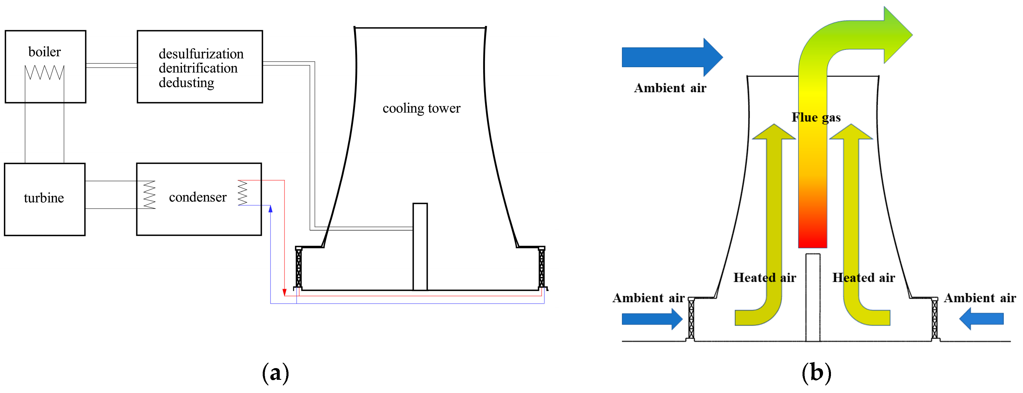
5]. After desulfurization, the flue gas temperature can be reduced to about 50 ℃, and the Froude number is not high enough to be discharged into the atmosphere directly. The general method is to reheat the flue gas through a gas-gas heat exchanger (GGH) [
6] and then introduce it into the chimney. However, reheaters can complicate the system and increase investment costs. Another method shown in
Figure 1 is to introduce low-temperature flue gas into cooling tower and discharge it through the thermal updraft of cooling tower. Therefore, the flue gas reheating system and chimney are eliminated in the natural draft dry cooling tower (NDDCT) with flue gas injection [
7]. Nevertheless, it should be noted that the inner shell surface area of cooling towers is much larger than that of traditional chimneys; thus, the cost of corrosion protection will increase greatly. Hence, it is significant to accurately predict the diffusion of flue gas in the cooling tower.
Accurate prediction of pollutant diffusion is one of the hot topics in fluid mechanics. Theoretical fluid mechanics uses mathematical methods to find out the quantitative results of problems. The research objects are usually linear problems or some specific nonlinear problems, while the governing equation of fluid mechanics is highly nonlinear; thus, it is very difficult to obtain its exact and analytical solutions through theoretical analysis. Experimental fluid mechanics plays an important role in fluid mechanics, but its disadvantages are also obvious, such as its long duration, high cost, difficult measurement, and only partially satisfying the similarity criterion. CFD is one of the most important technologies in the field of Fluid mechanics in the 21st century. The numerical simulation of NDDCT with flue gas injection is a very complex flow problem, involving atmospheric boundary layer, heat transfer, buoyancy drive, separation, pollution diffusion, and many other problems. Moreover, the large size of the cooling tower is in sharp contrast to the small size of the radiator, which makes the simulation very difficult. In recent years, numerous published studies focus on flue gas diffusion in coal-fired power plant based on CFD method. Klimanek et al. [
8] found that the increasing wind speed caused the formation of recirculation regions of flue gas flow near the tower outlet increasing the risk of corrosion of tower shell by numerical modeling of NDDCT with flue gas injection. Jahangiri [
9] incorporated the flue gas duct in NDDCT modeling and found the flue gas injection with wind breaking wall caused enhancement on the sucked air flow rate and the radiator heat rejection and thus the overall performance under crosswind conditions. Numerical simulation of NDDCT conducted by Eldredge et al. [
10] revealed that among various flue gas related variables the flue gas temperature was the key variable affecting tower performance through the buoyancy effects. Ma et al. [
11] developed a coupled model with three-dimensional (3D) CFD for NDDCT in junction with thermal calculations for turbine condenser, and provided reliable predictions of operation strategy for better performance under various ambient temperature and crosswind. Schatzmann et al. [
12] found that for most cases, such as low wind speed and moderate wind speed, flue gas discharged by cooling tower is better than the traditional chimney; the traditional chimney smoke performs better only in a few strong wind conditions. Yang et al. [
13] applied the CFD method to simulate the distribution of pollutants such as gaseous pollutants and particulate matter from flue gas emissions in a coal-fired power plant. The emissions were studied in a natural draft cooling tower with flue gas injection and a chimney. The results indicated that natural draft cooling tower with flue gas injection is more appropriate for flue gas emission than chimney.
Compared with aviation, construction, bridge and other fields, the simulation of NDDCT with flue gas injection is a relatively new problem. Therefore, the research findings of numerical simulation of NDDCT with flue gas injection are far less abundant than aerospace and wind engineering, and the research depth is relatively shallow. Thus far, as shown in the previous literature, most of the studies on numerical simulation of pollutant diffusion in NDDCT with flue gas injection are all based on the RANS model. However, with the improvement of computing power, LES with the capability of better dealing with turbulence fluctuations has become a promising and preferred methodology to simulate various turbulent flow phenomena [
14,
15,
16]. LES shows better agreement with experimental results than RANS in terms of the distributions of mean velocity and turbulence energy around simple buildings [
17,
18,
19]. Tominaga and Stathopoulos [
20] investigated the flow dynamics and pollutant dispersion in a simple three-dimensional street canyon by comparing RANS (RNG
k-ε) and LES, and found that LES yielded better results than RNG
k-ε in modeling the distribution of mean concentration by comparison with wind tunnel experiments. Better performance for LES against RNG was also achieved in the representation of turbulent scalar flux when the modeling system extended to a building array with a point source primarily due to the problematic turbulent Schmidt number in RANS model for scalar transport in complex flow fields [
21]. Gousseau et al. [
22] applied both RANS (Standard k-ε) and LES to simulate pollutant dispersion in actual urban building groups, and LES showed a better performance with the advantage of solving the dispersion equation without any parameter input, as the mass diffusivity of subgrid-scale was computed with a dynamic procedure Although the calculation accuracy of LES is higher than that of RANS, the calculation cost is also higher than that of RANS, which is one of the reasons for restricting the large-scale application of LES. A new class of turbulence simulation methods, the hybrid RANS/LES method, can effectively balance the computational cost and simulation accuracy by using RANS and LES in different areas of the flow field. Fröhlich and Terzi [
23] reviewed the recent researches on the coupling of RANS and LES, and introduced and verified the methods in detail. The results show that the hybrid method can combine the advantages of RANS and LES well and avoid the disadvantages of both, and has great potential in practical application.
A large number of researches show that LES is in better agreement with experimental results because it can predict turbulence fluctuations more accurately. However, literatures on numerical simulation of pollutant diffusion in NDDCT with flue gas injection are all based on RANS model, and there are only a few reports of simulations using LES. In view of this, two models, RANS and LES, are adopted in this paper to simulate the flue gas diffusion for NDDCT with flue gas injection under same working condition. By comparing the differences of equations and flow field characteristics of the two methods, the differences of pollution diffusion characteristics are analyzed. The final results are intended to provide a reference for pollution emissions in the energy industry.
The present paper is organized as follows.
Section 2 introduces the methods, research object and relevant software settings adopted in this paper, appropriate examples are selected to verify the reliability of the method. In
Section 3, the obtained results are presented and discussed. RANS and LES are compared from the aspects of cooling tower performance, internal and external flow field and pollutant concentration field inside and outside the cooling tower. Taking the time history of flow field parameters as the starting point, the gap between the two methods in capturing transient wave motion is analyzed.
Section 4 summarizes the essential findings of this work.
2. Materials and Methods
ANSYS FLUENT (version 15.0) [
24] was selected as the CFD tool to simulate the flow and pollutant fields of the NDDCT with flue gas injection in this study, and both RANS Realizable
k-ε and LES approaches were applied. The flow was assumed as incompressible, turbulent, and continuous. After being heated by the cooling tower radiators, the air temperature rises and the density decreases. Under the action of buoyancy, the hot air flows upward, thus driving the airflow in the cooling tower.
2.1. Numerical Approaches
The mathematical equations of RANS and LES are described in many literatures [
18,
25]; only a brief introduction to these two approaches is presented here. Equations 1 and 2 are the momentum equations of RANS and LES, respectively:
The overbar in RANS represents time averaging, and the wavy line in LES represents filtering. The idea of RANS is to average the Navier-Stokes (NS) equation and transform the unsteady turbulence problem into a steady problem, at the cost of an additional unknown, called Reynolds stress, which is in Equation (1). The idea of LES is to filter the NS equation, use a direct numerical simulation for large scale turbulence, and describe the turbulence smaller than the filter scale with some model. Mathematically, turbulence smaller than the filter scale is represented by an additional stress term called subgrid-scale stress, which is in Equation (2). On the surface, the two equations look very similar. However, LES can still simulate unsteady turbulence essentially, but at a much wider scale. However, RANS abandoned the simulation of unsteady turbulence information and only sought the flow results in the average sense. The two approaches start from completely different points of view.
In RANS simulations, the Realizable
k-ε [
26] was employed, and the standard Smagorinsky model [
25] was used for the sub-grid scale eddy viscosity model in LES simulations. Descriptions of Realizable
k-ε and LES approaches have been mentioned in many literatures [
19,
27], which will not be repeated here. The default values were used for the relevant settings in ANSYS FLUENT. Transient computation is necessary for LES model, and the time step was set to 0.1 s. To remove the influence of initial conditions, 500 s (5000 time steps) was firstly promoted to reach a relatively stable state. Then, time averaging was conducted for 1000 s to obtain statistical values, and it was confirmed that the statistical values remain unchanged over time. The pressure-based segregated algorithm Semi-Implicit Method for Pressure Linked Equations (SIMPLE) was used to deal with pressure and velocity. The second order upwind method was applied to discretize the momentum, turbulent and energy equations. For LES simulation, the bounded central differencing method was used to discretize the momentum equation. Convergence was assumed when the scaled residuals drop to the order of 10
-5 or the monitored variables (mass-weighted average temperature at the exit plane of the cooling tower outlet and the air mass flow rate of the cooling tower) remained stable [
27].
2.2. Configuration of NDDCT with Flue Gas Injection
In this study, the NDDCT of a 660 MW coal-fired unit was adopted as the research object. The flue gas stack was simplified to a cylinder and placed in the center of the NDDCT. The main dimensions of cooling tower and stack are shown in
Figure 2. The number of cooling deltas was 180.
2.3. Mesh and Boundary Condition
As shown in
Figure 3, the computational domain is set as cylinder with a 1700 m height and a 1700 m radius, which is discretized by structured hexahedron mesh [
28], and the minimum mesh size was set to be 0.4 m. The total number of mesh cells is about 5.7 million, and the mesh sensitivity analysis showed that less than 0.4 % deviation of mass-weighted average temperature of at the exit plane of cooling tower outlet and the air mass flow rate of the cooling tower could be reached when the number of mesh cells is over 5.7 million.
Figure 4 shows the mesh for NDDCT with flue gas injection.
The ground and the surface of cooling tower were assumed to be no-slip and adiabatic boundary conditions. The boundary conditions at the leeside and top of the computational area were the pressure outlet; the boundary condition of windward side was the velocity inlet, with the form defined as:
where
z is height. In this study,
Ur = 4 m/s was the velocity at the referred height (10 m), and the wind profile index
α was assumed as a typical value of 0.2. The turbulent kinetic energy
k and the turbulent dissipation rate
ε were set following the guidelines provide by Tominaga et al. [
29] in both Realizable
k-ε and LES. The vortex method was adopted for generating the fluctuating inlet boundary in LES, and the number of vortexes was the default value of 190.
The heat exchanger bundles were the heat source and the main source of resistance for the cooling tower, but the size of heat exchanger bundles was so small that it is almost impossible to fully simulate the details. [
30]. In this study, the heat exchanger bundles were simplified into the radiator model [
31]. The pressure drop Δ
p across radiator was defined in the form:
where
ρ is the air density,
v is the airflow velocity in the normal direction of the radiator, and
kL is the non-dimensional loss coefficient, defined as:
where
N is set to 2 and
rn are polynomial coefficients defined as
r0 = 48.675,
r1 = – 6.305,
r2 = 0.299 [
8].
The heat transferred to the air by the radiator is obtained by the following equation:
where
Text and
Tair,d are the temperature of the radiator and the air downstream of the radiator, respectively.
h is the convective heat transfer coefficient, defined as:
where
N is set to 2 likewise,
h0,
h1, and
h2 are set to 17,683.43, -9167.38, and 1938.02, respectively [
8]. It should be noted that the purpose of this paper was to compare the performance of RANS and LES in pollutant diffusion simulation transversely, thus, the relevant parameters did not need to be very accurate, as long as they were within a reasonable range.
2.4. Parameters of Ambient Air and Flue Gas
The real flue gas contains SO2, NOx, CO2, etc. SO2 was only simulated, since no chemical reactions were considered in this study. Thanks to ultra-low emission transformation, the average SO2 emission concentration of the large coal-fired units of the China Energy Investment Corporation was about 20 mg/Nm3 (approximately equal to 7 ppm). The boundary condition of flue gas injection outlet was set as the mass flow rate with a value of 929.753 kg/s, and the temperature of flue gas was set to 50 ℃. It was assumed that the parameters of the injected flue gas are the same in all of the cases.
2.5. Model Validation
Since limited field measurements of NDDCT with flue gas injection were available, the constructed model was validated against recently published relevant data on the heat transfer in NDDCT and pollution dispersion in street canyon in the following procedure. The computational accuracy of CFD method in heat transfer of NDDCT was firstly verified by comparison with the results by Li et al. [
27], and then the simulation ability of pollutant diffusion was verified against experimental and simulation data by Tominaga et al. [
20].
Figure 5 shows the comparisons of the simulation and literature results. In
Figure 5a, the simulated results are in good agreement with those in the reference. In
Figure 5b, there are some differences between the simulation results in this paper and those in the reference, which may be due to the differences in the definition of computational domain and mesh generation between this paper and references. However, the trend of the two results is basically the same, and the high accuracy of LES is also reflected. This conveys that the numerical model has a good computational accuracy in the simulation of both heat transfer and pollution dispersion and can be used for further study.
3. Results and Discussion
Steady Realizable k-ε (hereafter referred to as RANS), unsteady Realizable k-ε (hereafter referred to as URANS) and LES were used to simulate and analyze the flow fields and concentration fields inside, at the outlet and outside of the NDDCT with flue gas injection.
3.1. Performances
Figure 6 shows the time evolutions of air mass flow rate and heat rejection of cooling tower by URANS and LES. It can be seen that the air mass flow rate and heat rejection of cooling tower obtained by URANS were slightly higher than those obtained by LES, and the fluctuation of URANS was very small compared with LES. Both URANS and LES showed a highly similar trend of mass flow and heat dissipation over time.
Discrete Fourier Transform (DFT) can be used to obtain the amplitude spectrum of any signal that changes with time. Taking mass flow rate as an example, the amplitude spectrum after DFT is shown in
Figure 7. It should be noted that the amplitude spectrum here has filtered out the dc part (i.e., the signal with a frequency of 0). Firstly, it can be seen that the maximum amplitude value in the amplitude spectrum of URANS simulation results was much smaller than LES. Secondly, with an increase of frequency for URANS, the amplitude decreases monotonically, while the frequency with the largest contribution in LES was the sub-low frequency 0.00244 Hz. The airflow through the cooling tower was directly related to its internal and external velocity distribution. The mass flow rate of URANS fluctuated very little, which means that the flow field obtained by URANS simulation was very stable and close to a steady flow. However, the mass flow rate of LES fluctuated greatly, indicating that LES can capture the unsteady information that cannot be obtained by URANS.
3.2. Inside of Cooling Tower
Figure 8,
Figure 9 and
Figure 10 are contours of velocity, pressure and pollutant concentration distribution in the vertical plane of, respectively, all values; if not specified in URANS and LES, simulations were time averaged. It can be seen that the simulation results of RANS were almost the same as URANS. However, LES presented different results at the bottom, outlet downwind and downstream of cooling tower.
Figure 8 shows that all three methods can simulate the separation at the inner wall near the radiator and the lee side of the cooling tower. However, the leeward speed ranges of cooling tower in RANS and URANS were significantly smaller than that in LES, which will affect the air mass flow rate of the downwind radiator. The difference of velocity distribution explains the diversity of mass flow rate between URANS and LES in the previous subsection. The velocity near the outlet of cooling tower was greater than that of LES, indicating that the mixture of flue gas and hot air was more sufficient in LES. This is because LES was far more capable of capturing unsteady flow than URANS, and turbulence can enhance mass and momentum exchange between different flows.
As can be seen from
Figure 9, there were some differences in the leeward pressure distribution of cooling tower obtained by RANS, URANS, and LES. Although the three methods can simulate the low-speed region on the leeward side of cooling tower, the leeward side pressure in the simulation results of RANS and URANS was significantly greater than that of LES. This is because the low-speed region simulated by RANS and URANS was not a separate flow, as a result of which, although the velocity of the flow field was very low, the pressure here can be recovered to a large extent according to Bernoulli’s equation. In the LES results, a low-pressure area appeared on the leeward side, and combined with the velocity distribution, it could be inferred that there is a separation flow here. The detailed flow field structure will be shown in the next sub-section.
Figure 10 shows the comparisons of temperature field distribution of cooling tower. The distribution of temperature field is mainly determined by the velocity distribution; thus, the temperature distribution of URANS and LES at the outlet of cooling tower was quite different. As can be seen from the
Figure 10, LES had a wider distribution range of hot air at the outlet of cooling tower, which indicates that the mixing of flue gas, hot air inside and cold air outside the tower was more intense at the outlet of cooling tower. Inside the cooling tower, heat and mass transfer were carried out between the heated air of the cooling tower and the flue gas discharged from the flue gas exhaust, including macroscopic convective motion and microscopic molecular thermal motion. Because LES has a better ability to simulate the details of the flow field, the flue gas and hot air mixed more fully, and the flue gas temperature dropped faster.
Vorticity can reflect the disturbance degree of the flow field to some extent, and the disturbance degree of the flow field affected the mass and energy transfer in the flow field directly.
Figure 11 shows the comparison of instantaneous vorticity for the three methods in the vertical plane. It can be clearly seen that LES simulated a lot of whirlpools, both inside and outside the cooling tower compared with RANS and URANS. RANS and URANS can only roughly simulate the velocity shear of flue gas and hot air and the separation flow above the radiator inside the cooling tower. LES could not only simulate the separation of upwind inside, bottom and downwind outside the cooling tower, but also capture the whirlpool generated by the velocity shear between flue gas and hot air. This explains the differences among the speed, pressure, and temperature of the three methods.
Figure 12 shows the concentration distribution of pollutants inside the cooling tower. The concentration value of RANS is the highest, and the diffusion range of pollutants in LES is the largest. The diffusion of pollutants is essentially heat and mass transfer, and its diffusion characteristics are determined by velocity and temperature distribution. The velocity distribution determines the macroscopic convective motion while the temperature distribution determines the microscopic molecular thermal motion. The distribution of temperature is closely related to the distribution of velocity, thus, in the final analysis, the distribution of velocity field had the greatest influence on the concentration field of pollutants. Velocity can be divided into average velocity and pulsating velocity superposition. The airflow movement is similar to the pipeline flow inside the cooling tower. Due to the same working conditions, the average velocity in RANS, URANS, and LES was basically the same, thus, the pulsation velocity becomes the key to affect the pollutant propagation. RANS can hardly capture the pulsation velocity, thus, the diffusion level of the flue gas is the lowest and the maximum value of concentration is the highest. Moreover, URANS could capture pulsation velocity only in large scales and low frequencies. Limited by the wall surface of cooling tower, the unsteady information obtained by URANS was very little. On the contrary, LES could not only simulate pulsation velocity with large scale and low frequency, but also capture pulsation with small scale and high frequency. Therefore, the diffusion of pollutants in LES was the most intense, with the lowest concentration of pollutants and the widest range.
Figure 13 shows the root-mean-square error (RMSE) of pollutant concentration calculated by URANS and LES. It is obvious that the pulsation amount in LES was much larger than that in URANS. This not only verifies that flow field pulsation has a great impact on pollutant diffusion, but also reflects that URANS lags far behind LES in capturing unsteady information.
Under the influence of ambient wind, the pollutant tended to approach the wall in the downwind direction of cooling tower. Once the flue gas touched the cooling tower wall, the risk of cooling tower wall corrosion was greatly increased.
Figure 14 shows the pollutant concentration in the inner shell of cooling tower simulated by three methods. For the convenience of observation, the 3D cooling tower inner shell surface was projected onto a two-dimensional (2D) plane. It can be seen that the results of LES were far better than those of RANS and URANS in terms of maximum value and range. In RANS, the maximum concentration of flue gas at the cooling tower inner wall surface was 0.0012 ppm, and the influence range of flue gas on the inner wall of cooling tower was roughly above throat and 1/4 downwind. The maximum flue gas concentration at the cooling tower inner wall surface in URANS was 0.0012 ppm too, and the influence range of pollutant at the cooling tower inner wall surface was slightly smaller than that of RANS. The maximum pollutant concentration in LES was 0.052 ppm, about 43 times that of RANS and URANS. The influence range in LES was approximately above 120 m downwind area, which was about 3–4 times of RANS and URANS. It can be seen that the results obtained by RANS and URANS are much more conservative than LES in the prediction of pollutants at the cooling tower inner wall surface.
3.3. Exit of Cooling Tower
In the previous sub-section, we mentioned that LES captured large pulsation when simulating flow field and pollutant concentration field; thus, we set several monitoring points at the outlet of cooling tower to observe the fluctuation of velocity and pollutant concentration. A total of five sampling points were set, and their numbers and coordinates are shown in
Figure 15.
Figure 16 shows the pollutant concentration distribution at the outlet of cooling tower. It can be seen that the maximum concentration in RANS was the highest, followed by URANS and LES was the lowest. This is closely related to the flow field disturbance in the cooling tower analyzed in the previous sub-section. The flow field inside the cooling tower in the RANS is very stable and fluctuates very little, so the concentration of pollutants decreases less, from 7 ppm to 2.5 ppm. Additionally, the flow field in URANS fluctuated slightly, thus, the concentration of pollutants decreased slightly from 7 ppm to 2.25 ppm. Additionally, the flow field fluctuated the most in LES, thus, the concentration of pollutants at the outlet of the cooling tower was the lowest, falling from 7 ppm to 1.75 ppm. Meanwhile, compared with RANS and URANS, the flue gas in LES was closer to the wall of cooling tower downwind, which is corresponding to the results in
Figure 14.
The streamlines near the outlet of the cooling tower are presented in
Figure 17. The cold ambient air from the outside and the mixed flue gas from the inside converge here. It can be seen that the two flows in RANS and URANS had a very obvious demarcation line, and the structure of the demarcation line was stable. In LES, the air outside and inside the tower were apparently mixed at the exit position with no demarcation line. It can be analyzed that the airflow in RANS and URANS still had a relatively stable flow pipe constraint after moving to the outside of the cooling tower, thus, the air mass flow rate of the cooling tower was quite stable. In LES, the flow of mixing zone near the outlet of cooling tower was extremely unstable. It is well known that the fluctuation of downstream will interfere with the flow of upstream in subsonic flow; hence, the air mass flow rate of cooling tower will fluctuate.
The RMSE pollutant concentrations at the outlet plane of cooling tower in unsteady simulations are shown in
Figure 18. The maximum fluctuation value of pollutant concentration in LES can reach 1.16 ppm, while the maximum value in URANS was 0.116 ppm, only about 1/10 of LES. It can be inferred that URANS was not as capable as LES in simulating unsteady flow. Meanwhile, it can be seen that the fluctuation range of pollutant concentration in LES was very close to the cooling tower shell, which corresponds to the high pollutant concentration in the cooling tower inner shell of LES in
Figure 14.
In
Figure 18, the pollutant concentration at Point 1 fluctuates, and the fluctuation at Point 3 is larger, while the pollutant concentrations at Point 2, 4, and 5 barely fluctuate. This indicates that the smoke basically will not diffuse to these three locations.
Figure 19 shows the fluctuation curve of pollutant concentration over time at monitoring Point 3 calculated by URANS and LES. Similar to the mass flow rate and heat rejection of cooling tower presented in
Figure 6, the pollutant concentration at Point 3 in URANS was basically a constant value, while the pollutant concentration at Point 3 in LES fluctuated strongly.
The time-domain velocity and pollutant concentration curves of Point 3 in LES were analyzed by spectral analysis in
Figure 20. For the convenience of observation, the dc signal in amplitude spectrum was shielded. As can be seen from the figure, the concentration amplitude of pollutant in Points 2, 4, and 5 was basically 0. Although the pollutant concentration amplitude in Point 1 was not 0, it was wondrously small. However, Point 3 shows that there was a strong signal of pollutant concentration and there were multiple frequency peaks of pollutant concentration
C, velocity magnitude
V and velocity component
w, which were 0.00122 Hz, 0.01099 Hz, and 0.01709 Hz, respectively.
Figure 21 shows the parameter correlation analysis at Point 3 in the LES results. It can be seen that the correlation between velocity magnitude
V and component
w was the strongest, while the correlation between various velocity components and between velocity component
v and velocity magnitude
V was almost zero. This is because the flow at the outlet of the cooling tower was mainly in the
z direction, supplemented by the
x direction, while there was nearly no flow in the
y direction. Compared with component
u and
v, the correlation between pollutant concentration
C and velocity magnitude
V and component
w was much stronger, proving that the diffusion of pollutants was determined by the local mainstream velocity.
3.4. Outside of Cooling Tower
In order to observe the diffusion characteristics of the flue gas after discharging the cooling tower more directly, five downstream sections were set, and the locations of sections from the center of the cooling tower were 100, 200, 300, 400, and 500 m, respectively. It should be noted that the flow inside the cooling tower could be regarded as a relatively stable pipe flow. However, the flow field outside the cooling tower was equivalent to the flow around a three-dimensional cylinder, which is a typical unsteady flow. Therefore, there may be a large error in the calculation results of RANS.
Figure 22 clearly shows the distribution characteristics of pollutant concentration in the downwind direction of the cooling tower. The pollutant concentration basically presents a horseshoe distribution. Unlike
Figure 16, the maximum concentration obtained by RANS simulation at the
x = 100 m section was the lowest: 0.145 ppm. That of URANS was slightly higher, 0.161 ppm, and showed a significant characteristic of high on both sides while low in middle. Moreover, LES had the highest concentration, 0.177 ppm. With the increase of the distance from the cooling tower, the pollutants in LES dissipated faster. At 500 m, the concentration range of pollutants in LES was smaller than that of RANS and URANS.
As discussed earlier, the concentration distribution of pollutants is closely related to the velocity distribution.
Figure 23 shows the instantaneous streamlines of the flue gas discharged from the stack simulated by different methods. It can be seen that the streamlines in RANS and URANS were basically symmetrical and smooth, while the streamlines in LES showed wave characteristics in the flow field. Considering that RANS is not well suited for simulating unsteady flow, it is understandable that the flow field parameters obtained by RANS and URANS were different. At 100 m downstream, the streamlines of RANS diffused to a range of 75 m in the
y direction and 20 m in the
z direction. The streamlines of URANS diffused in
y and
z directions with a range of 93 m and 28 m, respectively, and LES with a range of 46.5 m and 22 m, respectively. Obviously, the streamlines diffusion range of URANS was much larger than that of LES, thus, the maximum pollutant concentration of URANS in
Figure 22 was smaller than that of LES. Hence, the pollutant concentration did not decrease significantly in LES. On the contrary, pollutants in URANS were diffused to a greater extent, and the concentration decreased more.
Meanwhile, it can be seen that the streamlines on both sides of the URANS were denser than those in the middle. This is because when URANS is applied to a simulation, a pair of symmetrical vortices will be generated in the downstream of the cooling tower. The low pressure at the vortex center will suck pollutants to the vortex core. Therefore, the pollutant concentration of URANS in
Figure 22 was high on both sides but low in the middle.
Figure 24 shows the vorticity in
x direction at 100 m downstream; it is evident that there were a pair of symmetrical vortices in RANS and URANS. Although vortices also exist in LES and their intensity are larger, the scale of the vortices is smaller; additionally, the intensity and position of the vortices will change as the flow field progresses. On the whole, the stirring effect of flow field on pollutants in LES was not as strong as that of RANS and URANS.
Figure 25 shows the velocity vector of the 85 m height plane. Both RANS and URANS can only simulate the separation flow in a small area directly behind the cooling tower, which is obviously unreasonable. For a building of a large size, such as the cooling tower, the Reynolds number of external flow reaches an order of 10
7. Referring to the circular flow of the cylinder, there should be a supercritical flow behind the cooling tower here; that is, there exists a large range of separation and many irregular vortices. There were different levels of separation flow inside and outside the cooling tower in LES, which is more reasonable. The same problem can be seen in
Figure 26.
Figure 26 shows the pulsation of velocity in the
y direction outside the cooling tower at a height of 85 m. In the results of URANS, the RMSE
v was hardly observed, while it can be clearly obtained in LES. The fluctuation of lateral velocity
v proves that the vortex of alternating shedding exists in the downstream of cooling tower.
Figure 27 shows the ground pollutant concentration obtained by different methods. For the convenience of observation, the logarithmic treatment of the vertical coordinate was carried out due to the huge difference between the results. The ground pollutant concentration obtained by the three methods increased with the distance from the cooling tower. However, the maximum ground pollutant concentration in LES was about two orders of magnitude higher than URANS and about 11 orders of magnitude higher than RANS.
At a place far away from the cooling tower, the flow field was less disturbed by the cooling tower. On the premise of the same mainstream velocity, pulsation velocity played a decisive role in pollutant diffusion. In RANS and URANS, the independent variable of momentum equation was the time average velocity, and the pulsation of flow field was reflected by turbulent kinetic energy. However, turbulent kinetic energy is only reflected in the momentum equation as a source term; despite the use of unsteady simulation, the URANS model can only identify some pulsating flows with very large scales (such as the flow around buildings). However, the large-scale pulsation in the strict sense cannot be counted as the pulsation quantity. In LES, the independent variable of momentum equation is real-time velocity, thus, LES can simulate more details than URANS. This is why more and more people are using LES for flow field simulation.

 ,
, 