Abstract
This paper modeled the dry band formation and arcing processes on the composite insulator surface to investigate the mechanism of dry band arcing and optimize the insulator geometry. The model calculates the instantaneous electric and thermal fields before and after arc initialization by a generalized finite difference time domain (GFDTD) method. This method improves the field calculation accuracy at a high precision requirement area and reduces the computational complexity at a low precision requirement area. Heat transfer on the insulator surface is evaluated by a thermal energy balance equation to simulate a dry band formation process. Flashover experiments were conducted under contaminated conditions to verify the theoretical model. Both simulation and experiments results show that dry bands were initially formed close to high voltage (HV) and ground electrodes because the electric field and leakage current density around electrode are higher when compared to other locations along the insulator creepage distance. Three geometry factors (creepage factor, shed angle, and alternative shed ratio) were optimized when the insulator creepage distances remained the same. Fifty percent flashover voltage and average duration time from dry band generation moment to flashover were calculated to evaluate the insulator performance under contaminated conditions. This model analyzes the dry band arcing process on the insulator surface and provides detailed information for engineers in composite insulator design.
1. Introduction
Composite insulators have been extensively used to provide electrical insulation and mechanical support for high voltage (HV) transmission lines [1,2,3,4]. The shank of the composite insulator is made of fiberglass or epoxy, and the sheds of the composite insulator are made of composite materials. The hydrophobic nature of composite materials discretizes water into small droplets on the insulator surface and ensures good performance of insulators under contaminated conditions [5,6]. However, the humid pollution could form a layer under the severely contaminated environment and increase the leakage current density [7,8]. The leakage current generates heat and evaporates water in the pollutant layer to create the dry band [9,10]. The arc initializes due to the significantly increased electric field close to the dry band [11,12,13,14]. Theoretical models for dry band formation and arcing processes are valuable because they contribute to the investigation of composite insulator flashover mechanism [15,16] and provide detailed information for engineers to optimize insulator geometry.
B.F. Hampton first studied the formation of dry bands in 1964 [17]. E.C. Salthouse and J.O. Löberg introduced the specific process of dry band formation in 1971. In terms of surface resistivity and electric field, E. C. Salthouse pointed out that dry band formation is caused by energy dissipation [18,19]. J.O. Löberg concluded that the width and speed of dry band formation are related to the surface temperature [20]. The distorted distribution of the field strength of dry bands also plays an important role in dry band expansion [21,22]. By analyzing a 3-D insulator model with the finite element method (FEM), J. Zhou et al. gave the opinion that the distortion field strength increases the length of the dry band. The number of dry bands also influences the electric field distribution [21]. A. Das et al. summarized that the dry band position has a significant influence on the maximum electric field strength [22]. These studies present the characteristics of the dry band and analyze the effects of dry bands on electric field distribution and flashover phenomena. However, the process of dry band formation caused by leakage current and electric arc has not been investigated in detail. This paper proposes a model to analyze instantaneous electric and thermal field variation during the dry band formation and arcing processes. The fields were calculated using a generalized finite difference time domain (GFDTD) method.
The GFDTD method consists of the generalized finite difference method (GFDM) and the finite difference time domain (FDTD) method. The GFDM is a method improved from the finite difference method (FDM). The traditional FDM depends on mesh-dividing, which is not suitable for fields with complicated boundaries, while the GFDM is a meshless method to compute the relationship of any discrete point in the field of the boundary conditions. The GFDM has an advantage over traditional FDM in the sense that the density of the calculation points could be different according to the boundary conditions and precision required in the field domain. The concept of the GFDM was first put forward by J.J. Benito in 2001 [23]. L. Gavate et al. compared the GFDM with other methods and reviewed its application in fluid and force fields [24]. J. Chen et al. then calculated electromagnetic field using the GFDM to reduce the computation time [25]. Currently, GFDM has been used in field calculation problems such as heat transfer and fluid mechanics to increase the calculation accuracy of a relatively small area in a large field domain [26,27].
This paper analyzed instantaneous electric and thermal field distributions close to composite insulators and arcs. Finite difference time domain (FDTD) was utilized to investigate the characteristics of continuously changing fields. In 1966, K.S. Yee dispersed Maxwell’s equations with time variables using the method of discretization later-called Yee cell [28], which was gradually developed into FDTD. This paper investigated electric and thermal fields variation by combining the GFDM with FDTD. GFDTD is capable of increasing the calculation accuracy in a high precision requirement area and reducing the computational complexity in a low precision requirement area. The arc propagation and heat transfer processes are modeled based on the electric and thermal field distribution.
Many theories and laboratory experiments have demonstrated that the elongation of the insulator creepage distance is an effective way to increase flashover voltage, but it also increases the weight and reduces the mechanical stress endurance of the composite insulator. Therefore, recent studies have focused on insulator parameter optimization when creepage distances remain the same [29,30,31]. The simulation models proved that the flashover probability slightly increases with the insulator shank diameter and decreases with shed spacing [32,33,34]. The creepage factor (CF), shed angle, and the ratio of overhangs between alternating sheds are the factors that impact dry band formation and arcing processes on the composite insulator surface. These parameters were optimized in the paper to analyze the 50% flashover voltage and the average duration time from pollutant layer formation to flashover.
This paper investigated the mechanism of dry band arcing by simulating the processes of dry band formation and arcing under the influence of a heat transfer model and an arc propagation model. The simulation results were compared with the results of the experiment to verify the model. This paper optimized the composite insulator geometry when the creepage distances remain the same.
2. Model Schematic and Method
2.1. Insulator Model Schematic
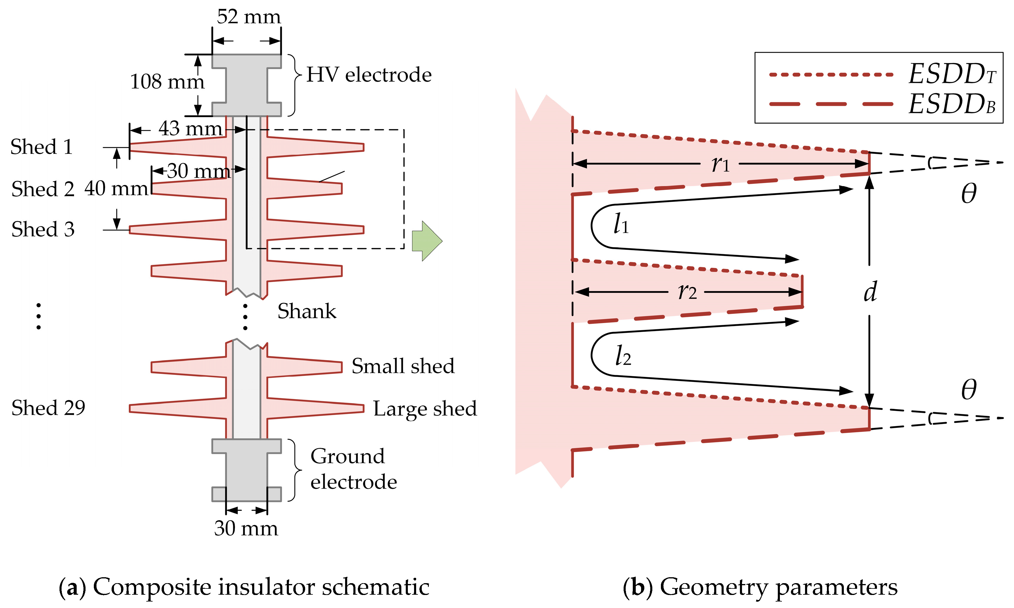
The composite insulator dimension and geometry were selected according to IEC 60815. Due to the symmetric geometry of composite insulators, a two-dimension model was applied to simulate the dry band formation and arc propagation processes and reduce the computational complexity. The composite insulators were designed for a 110 kV transmission line with 15 large sheds and 14 small sheds. The insulator shed radius and the dimensions of the electrodes are show in Figure 1a. The environment temperature and air pressure were 293 K and 101.325 kPa, respectively.
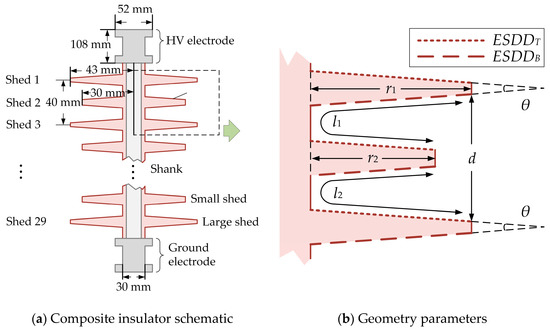
Figure 1.
Composite insulator model schematic.
In Figure 1a, the pollution distribution on the top and bottom surface of the insulator was defined as ESDDT and ESDDB. The flashover voltage reduces with the increase of the ratio of ESDDT to ESDDB. The range of the ratio was 0.1 to 1 [35]. In this paper, the ratio was set as 1 to simulate the dry band formation and arcing phenomena the under a severe polluted scenario with relatively low flashover voltage. Therefore, the ESDD value was 0.1 mg/cm2 and the surface resistivity is 8.3 × 10⁵ Ω·m under the influence of environment temperature and air humidity, and water particles in the air were not considered in the model [36,37].
In Figure 1b, θ is the shed angle. CF is defined as the ratio of the insulator creepage distance to the arcing distance.
where the sum of l1 and l2 is the total nominal creepage distance of the insulator. d is the arcing distance of the insulator.
r1 and r2 are the radius of large and small sheds respectively. kshed is defined as the ratio of r2 to r1.
In order to reduce the probability of dry band arcing and arc propagation, the geometry structure of insulator was optimized under the premise that creepage distances remain the same. The optimization variables of insulator geometry were CF, kshed, and θ.
2.2. Dry Band Formation and Arc Propagation Models
2.2.1. Electric Field and Arc Propagation Model
In the electric field close to the insulator, the Poisson is shown below:
where φ is the electric potential, ρc is bulk charge density and ε is permittivity.
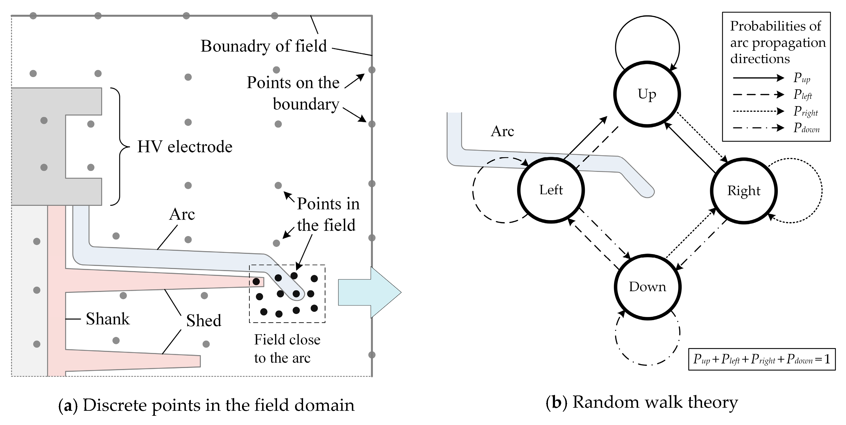
Before the arc ignition, the electric field calculation model computed the electric field distribution to determine the arc ignition and obtain the leakage current density on the insulator surface. After the arc ignition, the electric field and arc propagation model computed the instantaneous electric field strength around the arc leader during the propagation. The random theory was utilized to determine the arc propagation directions based on the instantaneous electric field.
The instantaneous electric field close to the composite insulator was calculated by the GFDTD method shown in Appendix A. The advantage of GFDTD is that the density of discrete calculation points could be different in the field domain according to the precision requirement and boundary conditions. To focus on the field close to the arc and reduce the computational complexity in the low precision requirement area, the distribution of points close to the arc is denser than the points distribution in other parts of the field (Figure 2a).
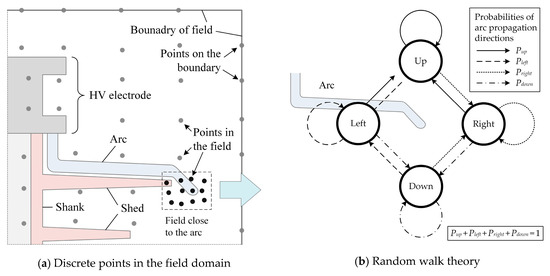
Figure 2.
Electric field calculation of the discretized points and arc propagation model based on the random walk theory.
Random walk theory calculated the probabilities of arc propagation in all the directions (Figure 2b). The random number was generated at each step of arc propagation to determine the exact direction of the next step. Therefore, the arc growth direction could be different even when the electric field distribution remains the same, which describes the stochastic characteristics of arc propagation [38].
where E is the electric field strength summation of all possible directions with E > Ec, and Ec (2.1 kV/mm) is the RMS value of the threshold field. a is the step function. The arc propagation velocity is in proportion to the magnetite of the electric field strength.
2.2.2. Heat Transfer Model
The heat transfer model simulates the energy balance of the evaporation process, including the leakage current injection energy, heat conduction and convection energies on the insulator surface, heat radiation energy of the arc, and the water evaporation energy of phase changing.
Before the arc ignition, the source of the thermal field was the accumulated energy on the insulator surface generated by the leakage current density. After the arc ignition, the heat transfer model included the heat radiation of the arc as the dominant factor to affect the dry band formation during arc propagation.
The leakage current injection energy is calculated as follows:
Heat conduction and convection are the main forms of heat dissipation on the composite insulator surface before arc initializes. Heat conduction partial differential equation (PDE) and boundary conditions are given as Equation (6).
where T is the thermal temperature, t is time, ρ, c and λ are the density, specific heat capacity and thermal conductivity of different insulating materials, respectively. Φ is the internal heat sources caused by dry band arcing and the leakage current density of the insulator surface.
The GFDTD method in the heat conduction calculation is similar to the electric field computation. The discretized heat conduction PDE is shown in Equation (7)
where the superscript “tn+1” represents the next stage in the discrete time domain.
Φ is calculated below:
where E is the electric field strength, J is the leakage current density and ρr is the resistivity of the insulator surface.
Thermal conduction and convection energies on the insulator surface are calculated below:
where l is the length of the insulator creepage distance, t0 is the time duration, λ is the thermal conductivity of the insulating material, is the thermal temperature on the insulator surface, ΔT is the temperature difference as a function of distance and time. T0 is the environment temperature. h is the heat transfer coefficient of convection.
Heat radiation becomes the dominant factor to cause heat transfer on the insulator surface after arc initialization. Heat radiation is the process of arc generating radiant energy. Arc radiation energy Warc_radiation is calculated below:
where εemit is the emissivity of actual objects, σ = 5.67 × 10⁻⁸ is the Stefan–Boltzmann constant, and t0 is the time period from the radiation start to the moment of field calculation.
Water in the pollutant layer evaporates during the heat transfer process. The Clausius–Clapeyron equation describes enthalpy variation based on air pressure and thermal temperature.
where Δ is the phase-changing enthalpy of water, R = 8.314 is the universal gas constant, P1 and P2 remain the same as the standard atmospheric pressure (101.325 kPa), and T1 and T2 are the thermal temperature change before and after arc initialization. Therefore, ΔH is a function of thermal temperature during the dry band formation and the arc propagation processes. The evaporation energy is calculated in Equations (13) and (14).
The thermal balance equation of dry band formation on the insulator surface is shown below:
3. Simulation Results
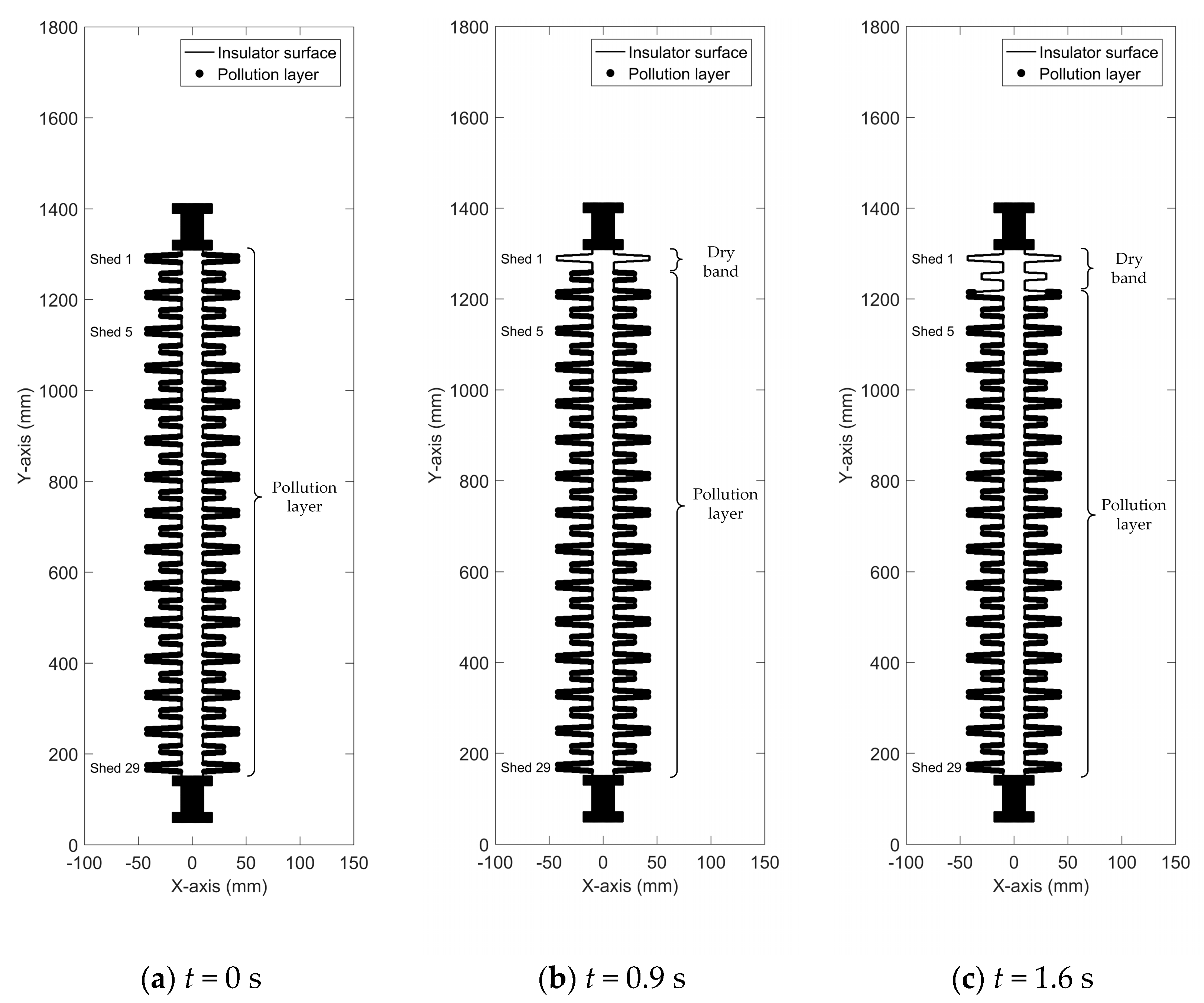
The dry band formation process from the moment of the insulator energization (t = 0 s) to the moment of arc initialization was simulated, in the first place, to analyze the effects of leakage current density on dry band formation. Then, the arc propagation process was simulated after arc initialization to investigate the effects of arc energy dissipation on further dry band formation and flashover.
3.1. Dry Band Formation and Arcing Simulations
The three stages of dry band formation before arc initialization are shown in Figure 3a–c respectively, when time t equals 0 s, 0.9 s, and 1.6 s.
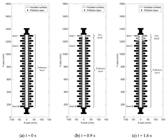
Figure 3.
Dry band formation process on the insulator surface at different time nodes.
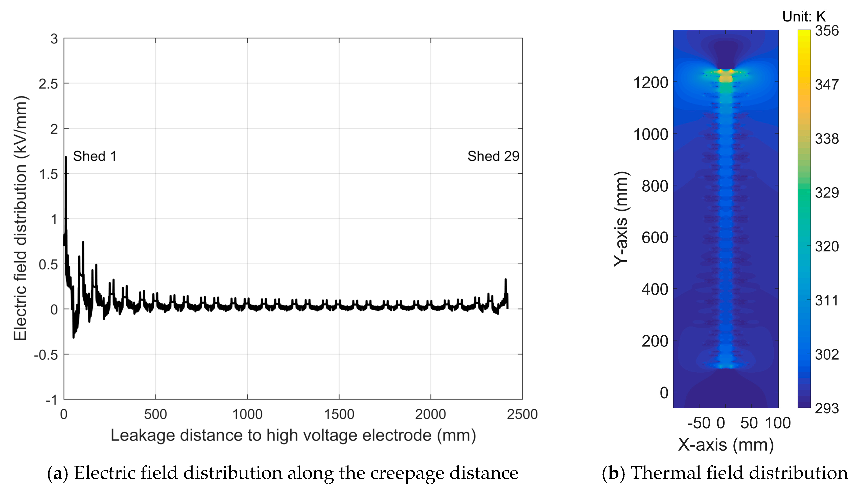
Figure 4 shows the electric and thermal field distributions at the initial state (t = 0 s) in Figure 3a before dry band formation. From Figure 3a and Figure 4b, it is evident that the dry band was first generated at the location with the maximum thermal field.
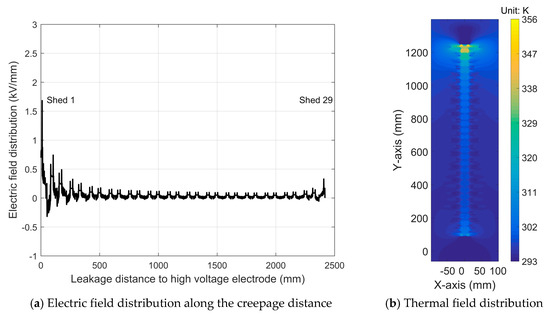
Figure 4.
Electric and thermal field distributions before the pollutant layer generation. (t = 0 s).
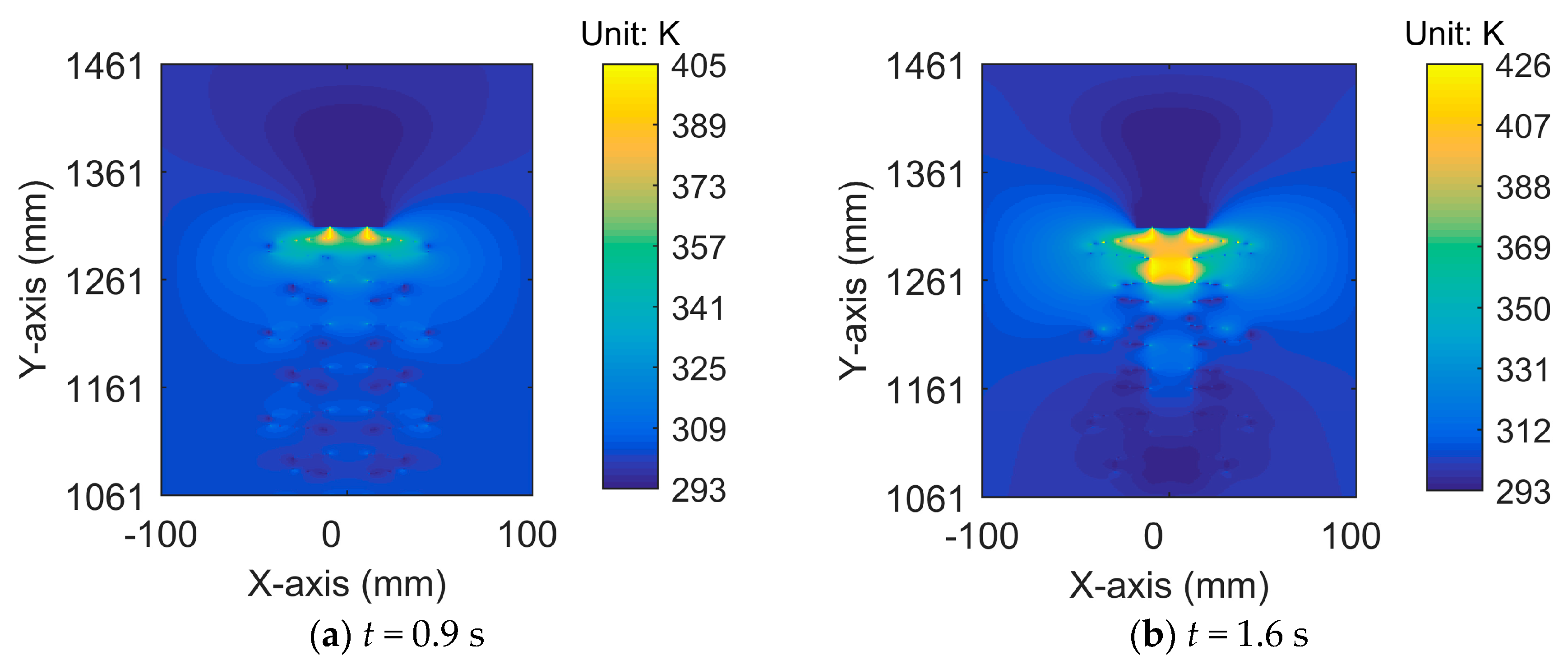
The dry band area expands as the water in the pollutant layer continues evaporating. The thermal field distributions on the insulator surface close to the HV electrode in Figure 3b,c are shown in Figure 5. Figure 5 indicates the mutual positive effects on thermal temperature and dry band length.

Figure 5.
Thermal field distributions close to the high voltage (HV) electrode when the length of the dry band increases.
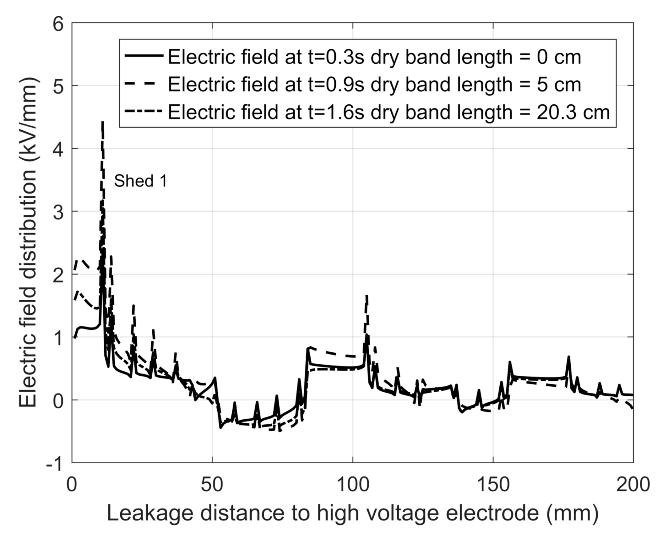
The electric field distributions on the insulator surface close to the HV electrode in Figure 3a–c are compared in Figure 6. Figure 6 shows that the maximum electric field with the dry band was higher than the maximum electric field without the dry band. The maximum electric field reduced when the dry band expanded.
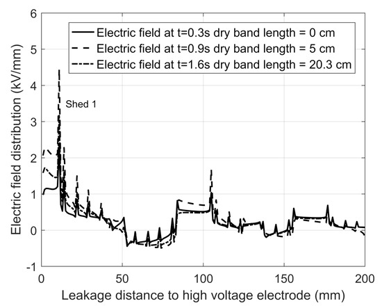
Figure 6.
Electric field comparison with different lengths of the dry band.
The arc initializes when the maximum electric field exceeds the dielectric strength of air. However, the arc did not ignite immediately in Figure 3b because the water evaporation consumed the energy so that the maximum electric field could not maintain above the dielectric strength of the air. The arc initialized at t = 1.6 s, even though the electric field reduced slightly due to the expansion of the dry band. (t = 5.42 s). The first arc initialization and the thermal field distribution are shown in Figure 7. Arc initializes at the location on the insulator surface with the maximum electric field. It is observed that the thermal temperature significantly increases when the arc ignites, the arc thermal radiation dissipates energy from arc to the air and insulator surface. The dominant factor of dry band formation becomes arc energy radiation during the propagation process. However, the arc extinguishes when the length and number of dry bands increase because the leakage current reduces as the surface resistivity at the dry band is dramatically higher than the resistivity at the pollutant layer.

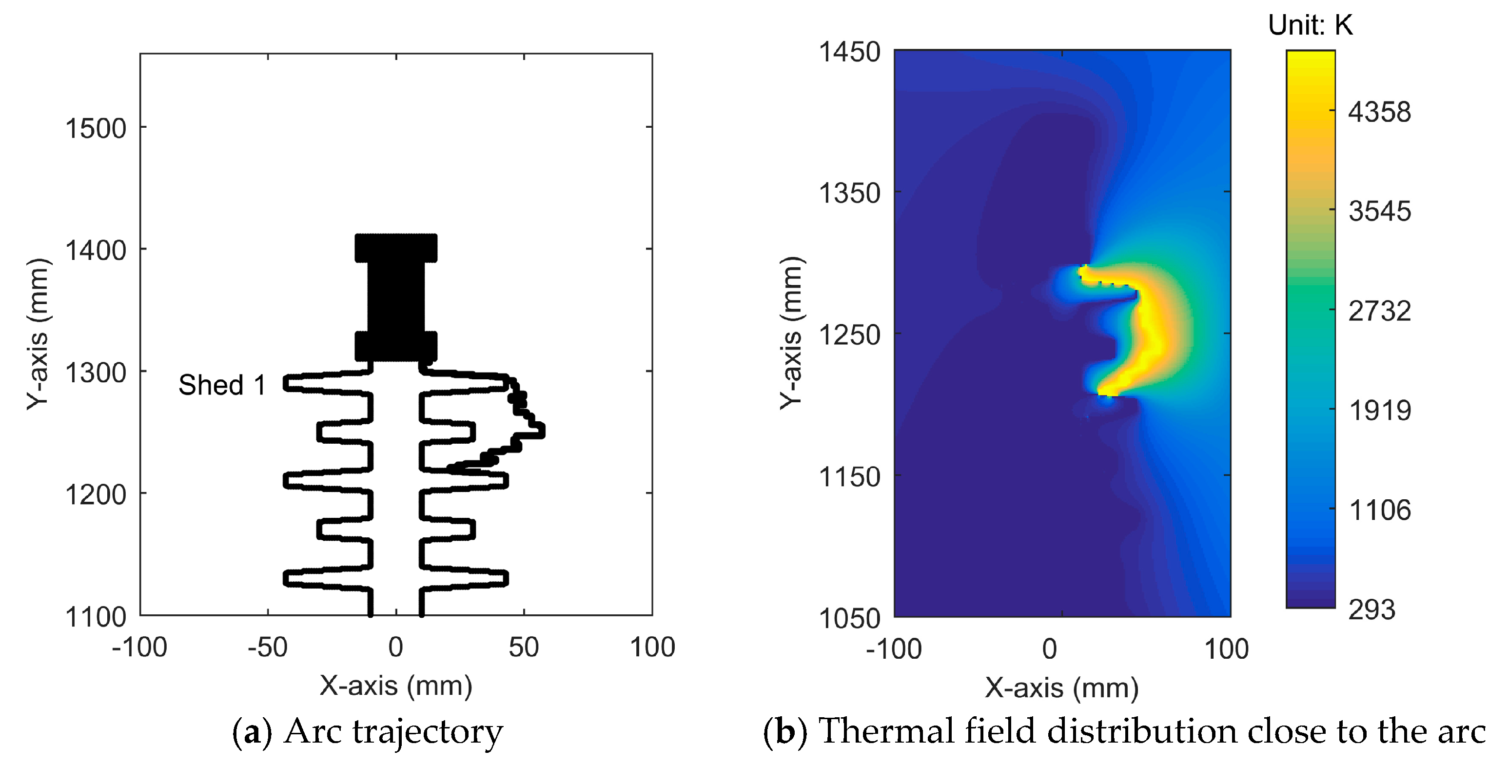
Figure 7.
Arc trajectory and thermal field distributions close to the HV electrode when the first arc ignites.
Two dry bands were generated during the arc propagation process. The dry band and thermal field distributions are shown in Figure 8a,b. The electric field distribution along the creepage distance is shown in Figure 9. Figure 9 shows that the maximum electric field was lower than the maximum field with one dry band in Figure 6. However, the electric field distortion along the creepage distance was more severe than the field distribution with fewer dry bands. The electric field at more than one location on the insulator surface exceeded the dielectric strength of air. Therefore, multiple arcs reignited at different places on the composite insulator surface.
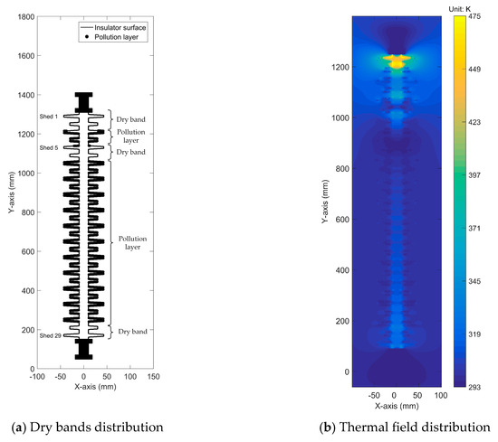
Figure 8.
Dry bands and thermal field distributions close to the HV electrode.
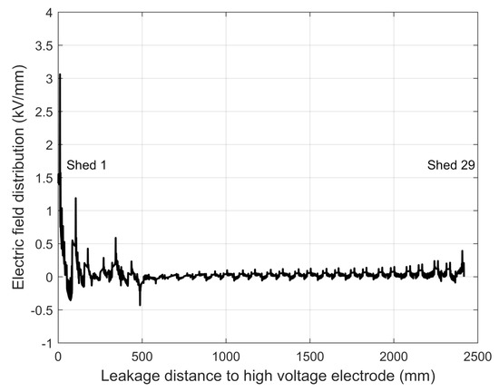
Figure 9.
Electric field distribution along the creepage distance with three dry bands on the insulator surface.
The distorted electric field led to the same distribution of the leakage current density. Therefore, temperature increased more significantly close to the dry band than the other locations on the insulator surface (Figure 8b).
Arcs ignited at different locations on the insulator surfaces after multiple dry bands generation when t was equal to 9.89 s (Figure 10a). Arcs distinguished with the expansion of dry band and ignited due to the distorted electric field close to dry bands. The iterations were repeated six times, and the number of arcs significantly increased after each iteration. The separated arcs were finally connected to a conductive path from the HV electrode to the ground electrode of the composite insulator and caused flashover (Figure 10b) when t was equal to 14.64 s.
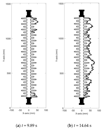
Figure 10.
Arc trajectory when multiple arcs occur and connect into a conductive path.
It was observed that the arc can jump between insulator sheds rather than traveling along the creepage distance. The arc trajectories could be slightly different due to the random walk theory. The arc jumping between sheds and stochastic characteristics in the model are consistent with the physical phenomena of the arc.
3.2. Experiment Results
The scheme of the experiment system is shown in Figure 11. Due to the hydrophobicity of the composite material, the insulator samples were coated with dry kaolin powder and NaCl to form the contamination layer [39]. The ESDD value of the contamination layer was 0.1 mg/cm2 to evaluate the dry band formation and arcing processes under a severely polluted scenario. The samples were firstly wetted by the clean fog and then energized with 110 kV at rated voltage to observe the dry band formation and arcing processes. The surface resistivity was 8.3 × 10⁵ Ω·m. The HV and ground electrodes had a diameter of 52 mm and a length of 108 mm as shown in Figure 1a. The high-speed camera (2F01) recorded 500 video frames per second at 800 pixels × 600 pixels from the start of the experiment to flashover. The videos were transmitted to the computer with 400 MB/s Ethernet.
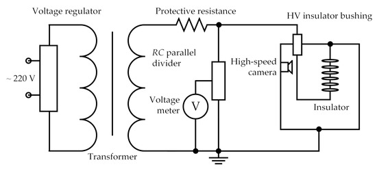
Figure 11.
The schematic of the dry band formation and arcing experiment system.
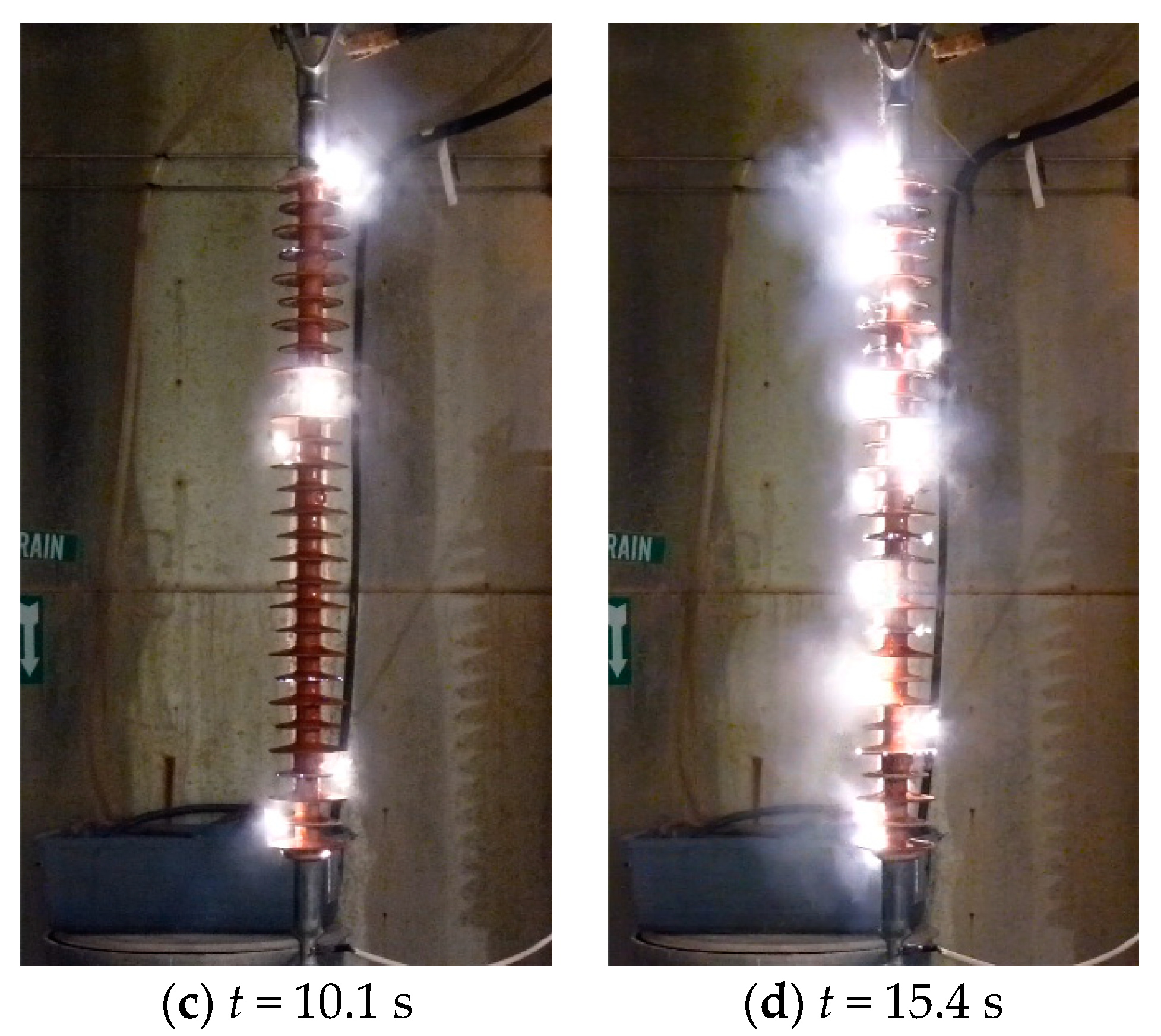
Figure 12 shows the experiment results of the dry band formation and arc propagation processes. The arc propagation at different time frames was compared to analyze the dry band location and arcing phenomena. Figure 12a shows the dry band formation process before arc ignition. Figure 12b shows the first arc ignition due to the dry band close to the HV electrode. Figure 12c shows the arcs reignite at different locations due to the presence of multiple dry bands on the insulator surface. Figure 12d shows that the separated arcs were connected and led to flashover. The time frames and phenomena are consistent with the simulation results in the model.
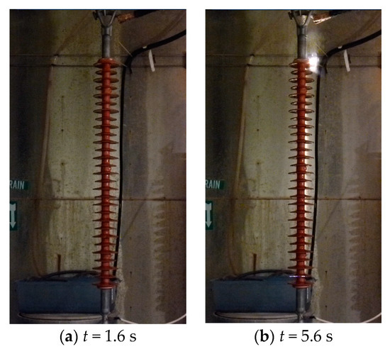

Figure 12.
The experiment results at different time nodes of dry bands formation and arc propagation processes.
The time nodes during arc propagation of the experimental and simulation results are compared in Table 1 to validate the simulation model.

Table 1.
Comparison of time nodes between experimental and simulation results.
4. Insulator Geometry Optimization
Since the experiment results verify the dry band formation and arc propagation model, three factors (creepage factor, shed angle, and alternative shed ratio) of composite insulator geometry were optimized in this section, while the creepage distance of the composite insulator remained the same as 2416 mm and the ESDD value was 0.1 mg/cm2. Due to the stochastic property of arc propagation, the dry band formation and arcing processes were repeated 187 times to calculate the 50% flashover voltage and average duration time from t = 0 s to the moment of flashover. The CF is defined as the ratio of insulator creepage distance versus the arcing distance. The shed angle is the angle of the shed surface slope. The alternative shed ratio is the ratio of the small shed radius to the large shed radius.
4.1. Creepage Factor Optimization
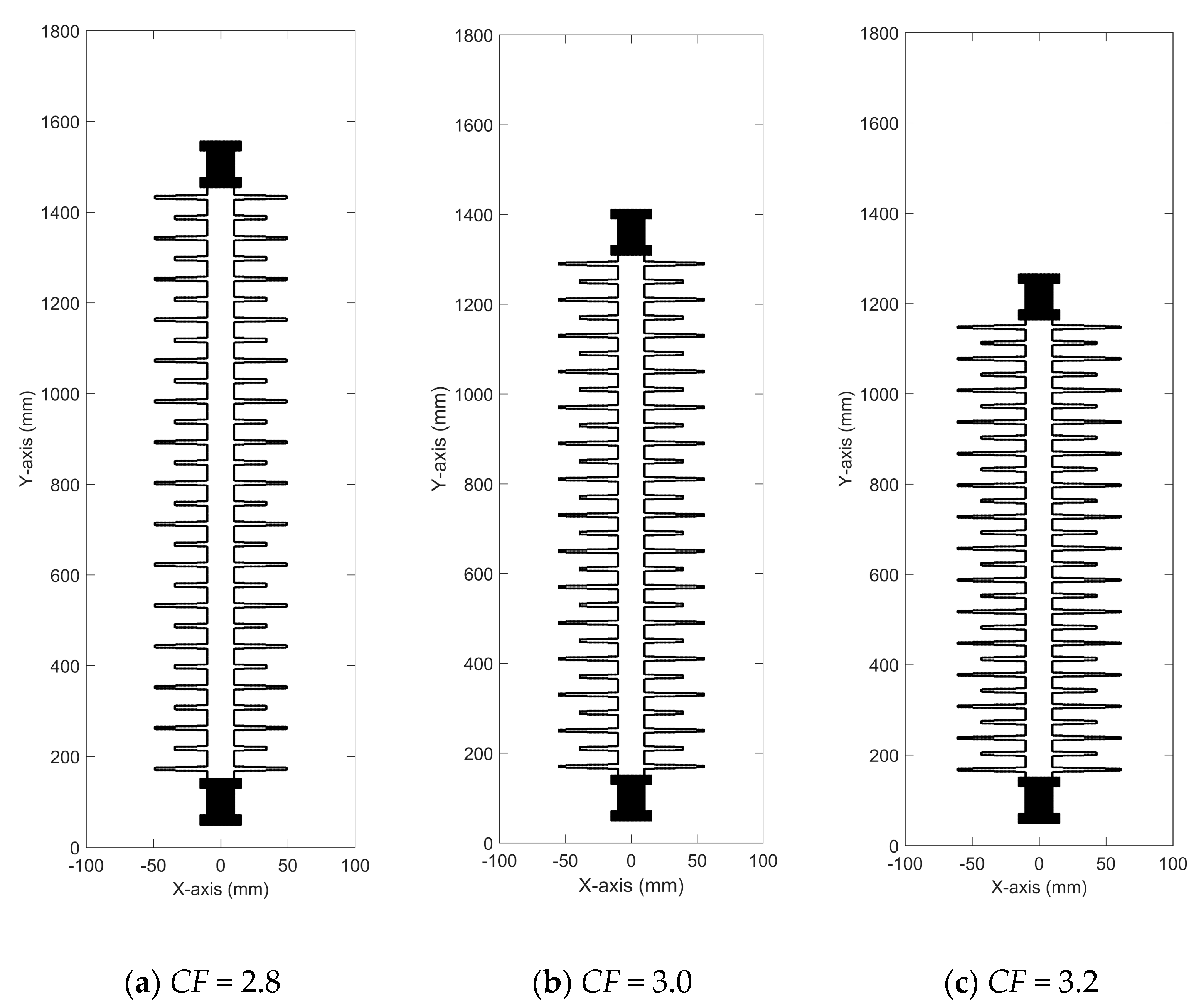
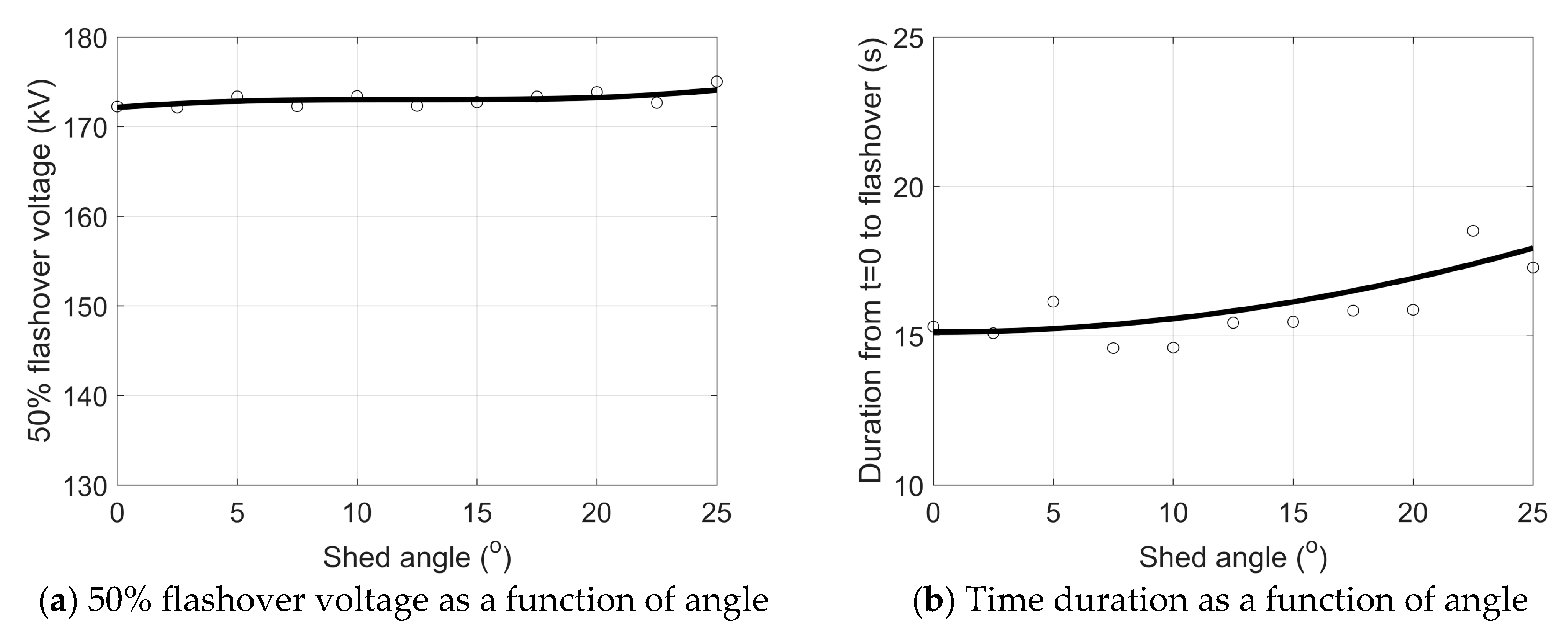
The CF was optimized when the shed angle was 10° and the alternative shed ratio was 0.8. The range of CF was from 2.5 to 3.5 according to IEC 60815. The insulator geometry with different CF values are shown in Figure 13. 50% flashover voltage and time duration as functions of CF value are shown in Figure 14. Figure 14 indicates that 50% flashover voltage first increased then reduced with the CF values. The optimal value of CF was 2.94 to achieve the minimum flashover voltage. The average duration time decreased with the CF values because the arc had a high probability to bridge sheds as the distance between sheds reduced with the increase of CF.

Figure 13.
Insulator geometry with different CF values (θ = 10° and kshed = 0.8).
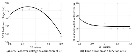
Figure 14.
50% flashover voltage and time duration as functions of the CF value.
4.2. Shed Angle Optimization
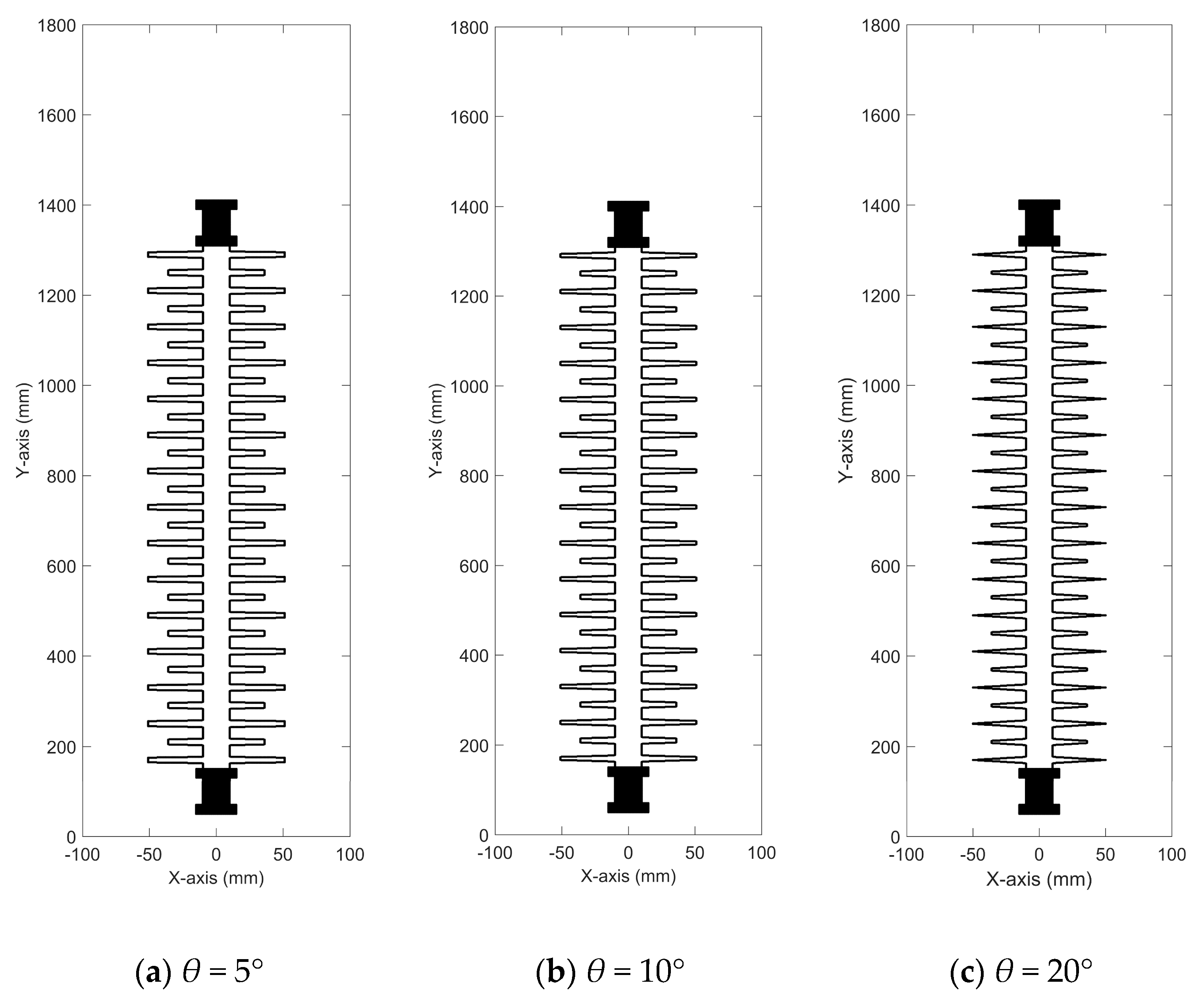
The shed angle was optimized when the CF value was 3.0 and the alternative shed ratio was 0.8. The range of shed angle was from 0° to 25° according to IEC 60815. The insulator geometry with different shed angles are shown in Figure 15. 50% flashover voltage and time duration as functions of shed angle are shown in Figure 16. Figure 16 indicates that shed angle had little impact on the 50% flashover voltage. The average duration time increased with shed angle because the average length of arc trajectories increased with shed angle.
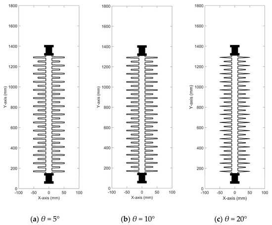
Figure 15.
Insulator geometry with different shed angles (CF = 3.0 and kshed = 0.8).
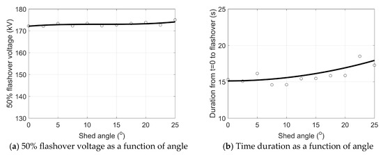
Figure 16.
50% flashover voltage and time duration as functions of the shed angle.
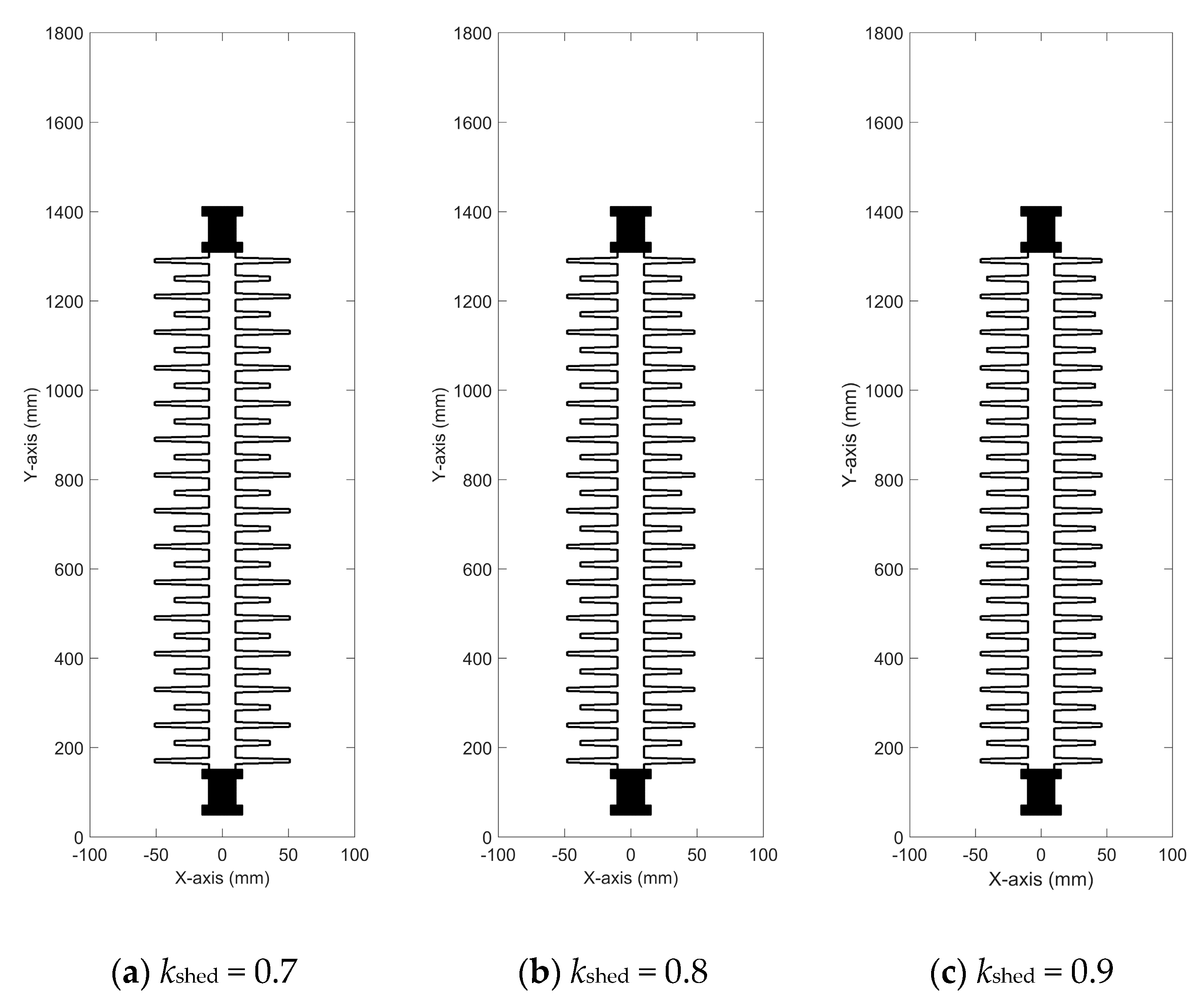
4.3. Alternative Shed Ratio Optimization
The alternative shed ratio was optimized when the CF value was 3.0 and the shed angle was 10°. The range of alternative shed ratio was from 0.7 to 1.0 according to IEC 60815. The insulator geometry with different alternative shed ratios are shown in Figure 17. 50% flashover voltage and time duration as functions of alternative shed ratio are shown in Figure 18. Figure 18 indicates that the 50% flashover voltage increased with alternative shed ratio because a small alternative shed ratio leads to the increasing occurrence of arc bridging between sheds. The alternative shed ratio had little impact on the average duration time.
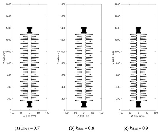
Figure 17.
Insulator geometry with different alternative shed ratios (CF = 3.0 and θ = 10°).
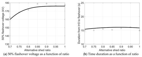
Figure 18.
50% flashover voltage and time duration as functions of the alternative shed ratio.
5. Conclusions
This paper modeled the dry band formation and arcing processes of polluted composite insulators. Instantaneous electric and thermal fields were calculated by the GFDTD method to investigate the mechanism of dry band arcing and flashover. The simulation results were verified by the laboratory experiments. Insulator dimension factors were analyzed to optimize insulator geometry when the creepage distances remained the same.
- The GFDTD method is suitable to calculate the electric and thermal fields for the insulator geometry by improving the field calculation accuracy at the high precision requirement area and reducing the computational complexity at the low precision requirement area.
- The stochastic characteristics and the arc trajectory jumping between insulator sheds were modelled to simulate the physical phenomena of the arc.
- The maximum electric field decreases with the expansion of the dry band. The heat transfer model demonstrates that the leakage current density is the dominant factor to affect dry band formation before the arc initialization, while the arc radiation becomes the dominant factor to form the dry band after the arc ignition.
- The 50% flashover voltage of composite insulators increases with the decrease of the CF value and the increase of the alternative shed ratio. The duration time from the pollution layer generation moment to flashover increases with the decrease of the CF value and the increase of the alternative shed angle.
Author Contributions
Conceptualization: J.H.; Methodology: J.H.; Software: J.H. and K.H.; Validation: K.H. and B.G.; Formal Analysis: J.H. and K.H.; Investigation: J.H.; Experiment: B.G.; Writing—Original Draft Preparation: J.H.; Writing—Review and Editing: J.H., K.H., and B.G.
Funding
This research was supported by the National Natural Science Foundation of China (Grant No. 51807028), the Basic Research Program of Jiangsu Province (Grant No. BK20170672).
Conflicts of Interest
The authors declare no conflict of interest.
Nomenclature
| A | coefficient matrix multiply with [Dφ] |
| (a−1)r,c | element at r-th row and c-th column of matrix [A]−1 |
| a(E − Ec) | step function of random walk |
| B | coefficient matrix multiply with [φ] |
| B(u) | residual function of two discrete points |
| b | constant matrix which equals to the product of [A] and [Dφ] |
| br, c | element at r-th row and c-th column of matrix [B] |
| c | specific heat capacity |
| CF | creepage factor |
| D | constant matrix which equals to the product of [A]−1 and [B] |
| Du | partial difference column matrix |
| d | insulator arcing distance |
| d1, 2, 3… | distance between two discrete points |
| dr, c | element at r-th row and c-th column of matrix [D] |
| E | electric field strength |
| Ec | RMS value of the threshold field |
| electric field strength in GFDTD form | |
| ESDDB | ESDD value of bottom part of the insulator |
| ESDDT | ESDD value of top part of the insulator |
| phase changing enthalpy of water | |
| h | heat transfer coefficient of convection |
| hij | absolute value X coordinate differences between two discrete points |
| J | leakage current density |
| leakage current density in GFDTD form | |
| kij | absolute value Y coordinate differences between two discrete points |
| kshed | ratio of radii of large and small sheds |
| l | length of insulator leakage distance |
| l1, l2 | insulator leakage distance |
| P | probability of random walk |
| P1, 2, 3… | discrete points |
| p1, p2 | saturated vapor pressure |
| R | universal gas constant |
| r1, r2 | radius of large and small sheds |
| T | thermal temperature |
| T0 | environment temperature |
| T1, T2 | thermal temperature change before and after arc initialization |
| t | time |
| t0 | time duration of insulator current leakage |
| u | column matrix of discrete point values |
| ui | value of field at a discrete point |
| V | volume |
| Warc_radiation | heat radiation energy of arcs |
| Wconduction | energy of heat conduction |
| Wconvention | energy of heat convention |
| Wleakage | energy of leakage current |
| Wwater_steam | required energy for water evaporation |
| w1, 2, 3… | weight function of discrete points in residual function |
| Γ | field boundary |
| ε | permittivity |
| εi | permittivity in GFDTD form |
| εemit | emissivity |
| θ | shed angle |
| λ | thermal conductivity |
| ρ | density |
| ρc | bulk charge density |
| bulk charge density in GFDTD form | |
| ρr | resistivity |
| σ | Stefan-Boltzmann constant |
| Φ | internal heat sources |
| Φi | internal heat sources in GFDTD form |
| φ | electric potential |
| electric potential in GFDTD form |
Appendix A
The GFDTD method is used to calculate the electric and thermal field distributions.
The advantage of GFDTD is that the density of discrete calculation points could be different in the field domain based on the precision requirement and boundary conditions.
According to the Taylor series expansion, the value of uj at point Pj of the function at near neighborhood of Pi is expressed as follows (Figure A1) [40]:
where hij and kij are absolute values of X and Y coordinate differences, i.e., hij = |xj − xi|, kij = |yj − yi|.
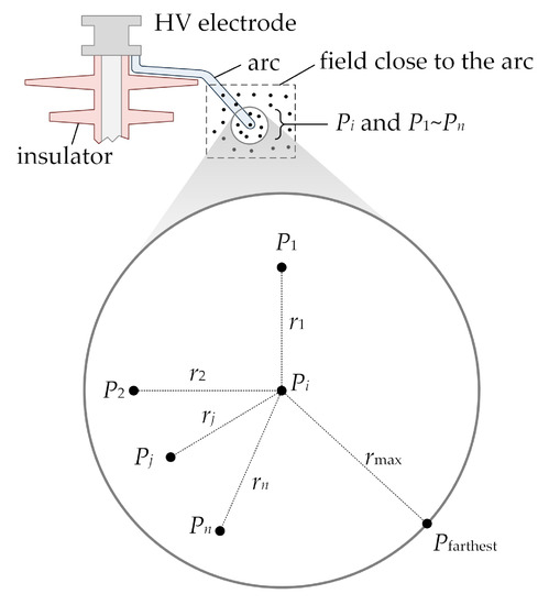
Figure A1.
Generalized finite difference time domain (GFDTD) in field calculation.
Figure A1.
Generalized finite difference time domain (GFDTD) in field calculation.
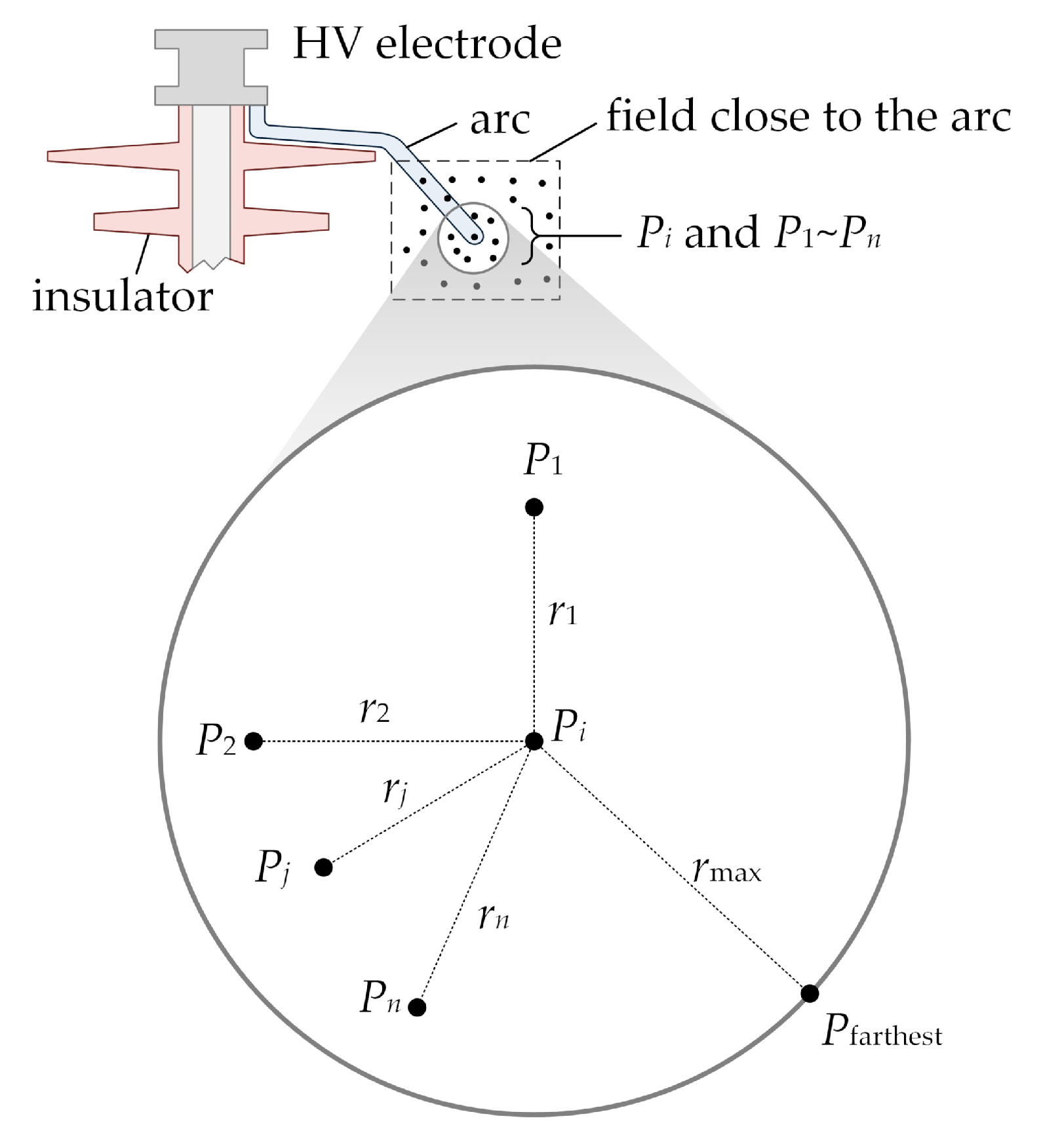
Pi is the point among P1~Pn. The value of each point Pi and P1~Pn is ui and u1~un. The distance from each point P1~Pn to Pi and is r1~rn, and the farthest distance is rmax.
The residual function of two points B(u) is defined by Equation (A3), shown as follows:
The weight function of the j-th point wj is calculated below:
Derive B(u) for ∂2u/∂x2 and ∂2u/∂y2, then get [A][Du] = [b], where matrixes [A], [Du] and [b] are shown as follows,
Decompose the matrix [b] as [b] = [B][u], where
The matrix [Du] is written in another form, i.e., [Du] = [A]−1[b] = [A]−1[B][u] = [D][u], where [D] = [A]–1[B] is a matrix with two rows and (n + 1) columns shown below:
where (a−1)r, c and br, c are the elements at r-th row and c-th column of matrix [A]−1 and [B].
Thus, ∂2u/∂x2 and ∂2u/∂y2 are written as
where dr, c is the element at r-th row and c-th column of matrix [D].
After substituting Equation (A11) into Equation (A1), the PDE is written as
where the superscript “tn” and “tn+1” are the present and next stages of the point u, respectively.
References
- Gorur, R.S.; Cherney, E.A.; Burnham, J.T. Outdoor Insulators; Ravi, S., Ed.; Gorur Inc.: Phoenix, AZ, USA, 1999. [Google Scholar]
- Gorur, R.S. Status Assessment of Composite Insulators for Outdoor HV Applications. In Proceedings of the 5th International Conference on Properties and Applications of Dielectric Materials, Seoul, Korea, 25–30 May 1997. [Google Scholar]
- Headley, P. Development and Application Experience with Composite Insulators for Overhead Lines. In Proceedings of the IEE Colloquium on Non-Ceramic Insulators for Overhead Lines, London, UK, 16 October 1992. [Google Scholar]
- Clift, S. Composite Fiber Optic Insulators and Their Application to High Voltage Sensor Systems. In Proceedings of the IEE Colloquium on Structural Use of Composites in High Voltage Switchgear/Transmission Networks, London, UK, 16 October 1992. [Google Scholar]
- Ilomuanya, C.S.; Nekahi, A.; Farokhi, S. Acid Rain Pollution Effect on the Electric Field Distribution of a Glass Insulator. In Proceedings of the 2018 IEEE International Conference on High Voltage Engineering and Application (ICHVE), Athens, Greece, 10–13 September 2018. [Google Scholar]
- Liu, Y.; Wang, J.; Zhou, M.; Fang, C.; Zhou, W. Research on the Silicone Rubber Sheds Performance of Composite Insulator. In Proceedings of the 2008 International Conference on High Voltage Engineering and Application, Chongqing, China, 9–12 November 2008. [Google Scholar]
- Hussain, M.M.; Farokhi, S.; McMeekin, S.G.; Farzaneh, M. Effect of Cold Fog on Leakage Current Characteristics of Polluted Insulators. In Proceedings of the 2015 International Conference on Condition Assessment Techniques in Electrical Systems (CATCON), Bangalore, India, 10–12 December 2015. [Google Scholar]
- Hussain, M.M.; Farokhi, S.; McMeekin, S.G.; Farzaneh, M. Mechanism of Saline Deposition and Surface Flashover on Outdoor Insulators near Coastal Areas Part II: Impact of Various Environment Stresses. IEEE Trans. Dielectr. Electr. Insul. 2017, 24, 1068–1076. [Google Scholar] [CrossRef]
- Hussain, M.; Farokhi, S.; McMeekin, S.G.; Farzaneh, M. Effect of Uneven Wetting on E-field Distribution along Composite Insulators. In Proceedings of the 2016 IEEE Electrical Insulation Conference (EIC), Montreal, QC, USA, 19–22 June 2016. [Google Scholar]
- Hussain, M.M.; Farokhi, S.; McMeekin, S.G.; Farzaneh, M. Dry Band Formation on HV Insulators Polluted with Different Salt Mixtures. In Proceedings of the 2015 IEEE Conference on Electrical Insulation and Dielectric Phenomena (CEIDP), Ann Arbor, MI, USA, 18–21 October 2015. [Google Scholar]
- Nekahi, A.; McMeekin, S.G.; Farzaneh, M. Ageing and Degradation of Silicone Rubber Insulators due to Dry Band Arcing under Contaminated Conditions. In Proceedings of the 2017 52nd International Universities Power Engineering Conference (UPEC), Heraklion, Greece, 28–31 August 2017. [Google Scholar]
- Qiao, X.; Zhang, Z.; Jiang, X.; Li, X.; He, Y. A New Evaluation Method of Aging Properties for Silicon Rubber Material Based on Microscopic Images. IEEE Access 2019, 7, 15162–15169. [Google Scholar] [CrossRef]
- Kim, S.H.; Cherney, E.A.; Hackam, R. Effect of Dry Band Arcing on the Surface of RTV Silicone Rubber Coatings. In Proceedings of the Record of the 1992 IEEE International Symposium on Electrical Insulation, Baltimore, MD, USA, 7–10 June 1992. [Google Scholar]
- Qiao, X.; Zhang, Z.; Jiang, X.; Liang, T. Influence of DC Electric Fields on Pollution of HVDC Composite Insulator Short Samples with Different Environmental Parameters. Energies 2019, 12, 2304. [Google Scholar] [CrossRef]
- Hussain, M.M.; Chaudhary, M.A.; Razaq, A. Mechanism of Saline Deposition and Surface Flashover on High-Voltage Insulators near Shoreline: Mathematical Models and Experimental Validations. Energies 2019, 12, 3685. [Google Scholar] [CrossRef]
- Hussain, M.M.; Farokhi, S.; McMeekin, S.G.; Farzaneh, M. Observation of Surface Flashover Process on High Voltage Polluted Insulators near Shoreline. In Proceedings of the 2016 IEEE International Conference on Dielectrics (ICD), Montpellier, France, 3–7 July 2016. [Google Scholar]
- Hampton, B.F. Flashover Mechanism of Polluted Insulation. Proc. Inst. Electr. Eng. 1964, 111, 985–990. [Google Scholar] [CrossRef]
- Salthouse, E.C. Dry-Band Formation and Flashover in Uniform-Field Gaps. Proc. Inst. Electr. Eng. 1971, 118, 630. [Google Scholar] [CrossRef]
- Salthouse, E.C. Initiation of dry bands on polluted insulation. Proc. Inst. Electr. Eng. 1968, 115, 1707–1712. [Google Scholar] [CrossRef]
- Löberg, J.O.; Salthouse, E.C. Dry-Band Growth on Polluted Insulation. IEEE Trans. Electr. Insul. 1971, EI-6, 136–141. [Google Scholar]
- Zhou, J.; Gao, B.; Zhang, Q. Dry Band Formation and Its Influence on Electric Field Distribution along Polluted Insulator. In Proceedings of the 2010 Asia-Pacific Power and Energy Engineering Conference, Chengdu, China, 28–31 March 2010. [Google Scholar]
- Das, A.; Ghosh, D.K.; Bose, R.; Chatterjee, S. Electric Stress Analysis of a Contaminated Polymeric Insulating Surface in Presence of Dry Bands. In Proceedings of the 2016 International Conference on Intelligent Control Power and Instrumentation (ICICPI), Kolkata, India, 21–23 October 2016. [Google Scholar]
- Benito, J.J.; Urena, F.; Gavate, L. Influence of Several Factors in the Generalized Finite Difference Method. Appl. Math. Model. 2001, 25, 1039–1053. [Google Scholar] [CrossRef]
- Gavete, L.; Gavate, M.L.; Benito, J.J. Improvements of Generalized Finite Difference Method and Comparison with Other Meshless Method. Appl. Math. Model. 2003, 27, 831–847. [Google Scholar] [CrossRef]
- Chen, J.; Gu, Y.; Wang, M.; Chen, W.; Liu, L. Application of the Generalized Finite Difference Method to Three-dimensional Transient Electromagnetic Problems. Eng. Anal. Bound. Elem. 2018, 92, 257–266. [Google Scholar] [CrossRef]
- Ureña, F.; Gavete, L.; García, A.; Benito, J.J.; Vargas, M. Solving Second Order Non-linear Parabolic PDEs Using Generalized Finite Difference Method (GFDM). J. Comput. Appl. Math. 2019, 354, 211–241. [Google Scholar] [CrossRef]
- Suchde, P.; Kuhnert, J.; Tiwari, S. On Meshfree GFDM Solvers for the Incompressible Navier–Stokes Equations. Comput. Fluids 2018, 165, 1–12. [Google Scholar] [CrossRef]
- Yee, K. Numerical Solution of Initial Boundary Value Problems Involving Maxwell’s Equations in Isotropic Media. IEEE Trans. Antennas Propag. 1966, 14, 302–307. [Google Scholar]
- Hou, K.; Li, W.; Ma, L.; Cheng, Y.; Jin, L. Multi-Objective Structural Optimization of UHV Composite Insulators based on Pareto Dominance. In Proceedings of the 2018 12th International Conference on the Properties and Applications of Dielectric Materials (ICPADM), Xi’an, China, 20–24 May 2018. [Google Scholar]
- Li, L. Shed Parameters Optimization of Composite Post Insulators for UHV DC Flashover Voltages at High Altitudes. IEEE Trans. Dielectr. Electr. Insul. 2015, 22, 169–176. [Google Scholar] [CrossRef]
- Doufene, D.; Bouazabia, S.; Ladjici, A.A. Shape Optimization of a Cap and Pin Insulator in Pollution Condition Using Particle Swarm and Neural Network. In Proceedings of the 2017 5th International Conference on Electrical Engineering-Boumerdes (ICEE-B), Boumerdes, Algeria, 29–31 October 2017. [Google Scholar]
- Liu, L. The Influence of Electric Field Distribution on Insulator Surface Flashover. In Proceedings of the 2018 IEEE Conference on Electrical Insulation and Dielectric Phenomena (CEIDP), Cancun, Mexico, 21–24 October 2018. [Google Scholar]
- Yu, X.; Yang, X.; Zhang, Q.; Yu, X.; Zhou, J.; Liu, B. Effect of Booster Shed on Ceramic Post Insulator Pollution Flashover Performance Improvement. In Proceedings of the 2016 IEEE International Conference on High Voltage Engineering and Application (ICHVE), Chengdu, China, 19–22 September 2016. [Google Scholar]
- Jiang, X.; Yuan, J.; Zhang, Z.; Hu, J.; Sun, C. Study on AC Artificial-Contaminated Flashover Performance of Various Types of Insulators. IEEE Trans. Power Deliv. 2007, 22, 2567–2574. [Google Scholar] [CrossRef]
- Jiang, X.; Zhang, Z.; Hu, J. Investigation on Flashover Voltage and Non-uniform Pollution Correction Coefficient of DC Composite Insulator. In Proceedings of the 2008 International Conference on High Voltage Engineering and Application, Chongqing, China, 9–12 November 2008. [Google Scholar]
- He, J.; Gorur, R.S. Flashover of Insulators in a Wet Environment. IEEE Trans. Dielectr. Electr. Insul. 2017, 24, 1038–1044. [Google Scholar] [CrossRef]
- Abd Rahman, M.S.B.; Izadi, M.; Ab Kadir, M.Z.A. Influence of Air Humidity and Contamination on Electrical Field of Polymer Insulator. In Proceedings of the 2014 IEEE International Conference on Power and Energy (PECon), Kuching, Malaysia, 1–3 December 2014. [Google Scholar]
- He, J.; Gorur, R.S. A Probabilistic Model for Insulator Flashover under Contaminated Conditions. IEEE Trans. Dielectr. Electr. Insul. 2016, 23, 555–563. [Google Scholar] [CrossRef]
- Pushpa, Y.G.; Vasudev, N. Artificial Pollution Testing of Polymeric Insulators by CIGRE Round Robin Method -Withstand & Flashover Characteristics. In Proceedings of the 3rd International Conference on Condition Assessment Techniques in Electrical Systems (CATCON), Chandigarh, India, 16–18 November 2017. [Google Scholar]
- Chan, H.; Fan, C.; Kuo, C. Generalized Finite Difference Method for Solving Two-Dimensional Non-Linear Obstacle Problems. Eng. Anal. Bound. Elem. 2013, 37, 1189–1196. [Google Scholar] [CrossRef]


© 2019 by the authors. Licensee MDPI, Basel, Switzerland. This article is an open access article distributed under the terms and conditions of the Creative Commons Attribution (CC BY) license (http://creativecommons.org/licenses/by/4.0/).