Abstract
To accomplish the limit protection task, the Min-Max selection structure is generally adopted in current aircraft engine control strategies. However, since no relationship between controller switching and limit violation is established, this structure is inherently conservative and may produce slower transient responses than the behavior by engine nature. This paper proposes an output-based limit management strategy, which consists of the safety margin module and the parameter prediction module to monitor system responses, plus the switching logic to govern switches between the main controller and limiters, and, in this way, a faster transient performance is achieved, and the limit protections in transient states become more effective. To realize smooth switching control, the linear-quadratic bumpless transfer method is developed. The design principle of the multi-loop switching control and bumpless compensator is detailed, and the effect—on limit protection control performance—of the design parameters in the safety margin and parameter prediction modules are also analyzed. The proposed approach is tested using simulations covering the whole flight envelope on the nonlinear component-level model of a turbofan engine, and the superiority over the Min-Max architecture is also validated.
1. Introduction
With the development of aircraft engine technology, higher demands on performance and functionality of electronic control systems have been required. It is known that performance promotion of aircraft engines can be obtained by larger shaft accelerations, which produce fast thrust responses. However, the accompanying change in aircraft engine aerodynamic and thermodynamic processes may incur several unsatisfying circumstances such as transient reductions in stall margin, large turbine temperature transients, the danger of compressor surge, and the increase in blade wear rate. Hence, critical engine variables are supposed to be maintained within permissible limits in order to ensure the operational safety of the aero-engine. Spang and Brown summarized that much of the complexity of control comes from the need to operate the engine as close as possible to the limits where engines are most effective [1]. Hence, the tradeoff between the high engine performance and operational safety should be taken into consideration during the design process of aircraft engine control systems.
Constraints—like temperatures, stall margins, and pressure ratios—should be considered as a part of a particular design process. For instance, considering stall margins, in order to avoid unstable aero-dynamic conditions—like surge or rotating stall—a sufficient surge margin in the worst operation condition was introduced in traditional design methods, despite the fact that these surges would not happen in all cases. This method contradicts the design philosophy of a control system, and the design convenience sacrifices dynamic performance.
In order to solve this problem, there are two main research approaches. One is multi-loop switching control method, which is represented by the Min-Max control strategy. In this method, the multiple loop control structure is adopted, and the control signals generated by each loop regulator are selected by using Min and Max selectors to ensure the safety of engine operation and realize the thrust control of the engine. In recent years, it has been widely used in commercial aero-engines [2,3,4,5]. For the Min-Max control strategy, current mainstream research interests mainly include the following three points: one is the controller design method to improve the control performance of the Min-Max scheme, such as applying a sliding mode controller to replace a linear controller to improve the limit protection control [6,7,8,9,10]. However, the changes proposed in this study necessitate a complete redesign of the engine controller, which will impose challenges in terms of verification across the whole operating envelope and acceptance by engine control implementers [1]. Some methods to shape the response characteristics of the engine outputs are to reduce the possibility of limit violation in the transient regime [11,12,13]; the second current research interest is to improve the switching logic of the Min-Max strategy, which can reduce unnecessary controller switching and improve the dynamic performance of the engine by adding information on key engine parameters as the basis of control loop switching [14]. Thirdly, is the stability verification of the Min-Max strategy, including the stability verification of the Min-Max control strategy with a sliding mode controller [15], and the substitution of Min and Max selectors with nonlinear equivalents, so as to transform the control system into the Lure’s system for stability verification [16]. However, it is undeniable that the Min-Max method has inherent shortcomings—i.e., its switching logic is only related to the control input. Although it can realize steady-state limit protection, it cannot achieve transient limit protection [3].
The other control method is based on the optimization algorithm, including model predictive controls and reference governors. For the former, because of its advantages in dealing with constraints, it is obviously suitable for dealing with limit management control problems of aero-engines, and a number of research results have emerged recently [17,18,19]. For the latter, its advantage is that it can keep the original control structure of the engine in service, optimize the control reference online by configuring an add-on scheme, and improve the limit management ability of the control system [20,21,22,23]. However, for the control method based on the optimization algorithm, its disadvantage is that the control effect depends on the accuracy of the prediction model, and the calculation complexity is too high to realize the control method in real-time. In addition to control methods, the mechanisms of engine unstable operating conditions (such as compressor surge, stall, etc.)—and the active control methods to deal with these—are “hot topics” to ensure the safety and stability of the engine. The author of [24] took a semi-historical look at some of these fields of study (stall, surge, active control, rotating instabilities, etc.) and examined the ideas which underpin each topic.
Unlike the Min-Max scheme, applying output-based switching logic in aero-engine limit management control is a new idea. However, if a direct switching method is adopted, it is likely to cause excessive disturbances in system parameters. Therefore, it is necessary to adopt a method to achieve smooth switching. Bumpless transfer is an approach to achieve smooth switching and has been extensively studied [25,26,27]. Green and Limebeer put forward a method to govern the off-line control signal to be as close as the on-line control signal by connecting a large gain in series in the feedback control loop of the off-line controller [28]. Hanus et al. proposed a bumpless transfer method [29] which was successfully applied in practical engineering projects such as the actual application in VSTOL (vertical and/or short take-off and landing) aircraft [30]. In recent years, compared with the traditional bumpless transfer method, the linear-quadratic bumpless transfer method proposed by MC Turner et al. has been widely used because of its advantages of fewer assumptions of controllers and no special requirements for system matrix [31,32,33].
This paper proposes an output-based bumpless transfer limit management method for aero-engines, in order to solve the issue that the Min-Max structure cannot establish a connection between the controller switching actions and limit violation. The switching logic of multiple engine control loops—based on a safety margin module and a parameter prediction module—was established. The linear-quadratic bumpless transfer method was exploited to restrain the oscillation of key parameters in the course of the direct switching of the control loops. A high-fidelity nonlinear component level low bypass ratio engine model was used as the controlled plant to carry out the numerical simulation. Based on the simulation results, the qualitative analysis of the influence of design parameters in the safety margin module and parameter prediction module on the control performance was carried out, which provides theoretical guidance for the selection of design parameters of the two modules in future research. The results of the control effect compared with that of the Min-Max structure showed that the proposed method possesses the ability to accomplish the limit control task, and has the advantages of avoiding premature controller switching, achieving faster transient performance in the whole flight envelope.
2. Output-Based Switching Logic of Multiple Control Loops
2.1. Multi-Loop Switching Control Strategy for Aero-Engines
The multi-loop switching control strategy is shown in Figure 1. Generally, multi-loop switched systems consist of a set of continuous (or discrete) time subsystems and a switching logic that decides how to switch between subsystems. The aim of this strategy is to solve the multi-objective control problem. For such problems, the key is the design of the controller and the switching logic. The former is mainly designed for its specific control objectives. For the latter, there are two design points: one is to select the switching signal reasonably; the other is to establish the connection between the switching signal and the activation index. Finally, the single-objective control of each subsystem is transformed into the multi-objective control of the system, and the multi-control loop is scheduled.
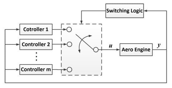
Figure 1.
Schematic diagram of multi-loop switching strategy.
The multi-loop switching control strategy of aero-engines is shown in Figure 2. is the control parameter, is the engine output parameter, is the switching logic signal and is the engine key parameter, where . represents the mapping of the engine key parameters to the engine output parameters and switching logic signals, namely . represents the mapping of the switching logic signals to the index of the activated control loop, namely .
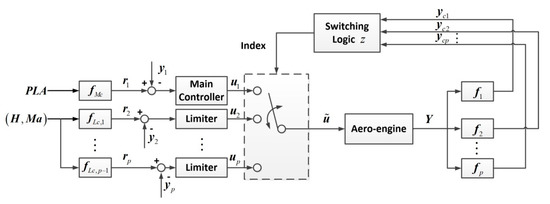
Figure 2.
Multi-loop switching control strategy for aero-engines.
In fact, the aero-engine limit management method is essentially to achieve multi-objective control tasks in an engine system. The property of the multi-objective is mainly embodied in the fast response requirement for the main control plan which is implemented by the main controller, and the security requirement for the limit control plans which are implemented by the limiters. The main control plan is obtained by mapping of PLA to the main output reference; the main output reference is often chosen to be the rotor speed. Limit control plans are obtained by mapping the of the flight condition to the output limit values; the limit outputs are often chosen to be the rotor speeds, pressures, and temperatures on the cross-section of the engine components, etc.
2.2. Output-Based Multi-Loop Switching Control Strategy for Aero-Engines
It can be seen that the design of switching logic is the key to realize a multi-loop switching control strategy from that mentioned above, and the following two points are mainly required to be considered in the design of switching logic: one is to select the engine signal needed by switching logic reasonably; the other is to design the mapping relationship from to . This section designs the switching logic based on the two points above.
Because the output-based limit management method of aero-engines proposed in this section is based on a multi-loop switching control strategy, according to the design points, the output of the engine is selected as the switching logic signal at first. However, if the current output is directly compared with the corresponding limit value, the corresponding limiter can only be activated when it exceeds or arrives at the limit boundary. Obviously, security is not well ensured by this method. Therefore, it is necessary to set a “safety margin” to determine whether the limit output is close to the restricted boundary. In addition, we still need to consider the current change rates of limit outputs and use these parameters to judge whether there is any risk of exceeding the limit in the future. Therefore, the key parameter of the engine, , is defined, which includes the engine output, , and the change rate of the output, . Based on this parameter, the safety margin module and the parameter prediction module are designed, respectively. Figure 3 shows the output-based multi-loop switching control strategy for aero-engine.
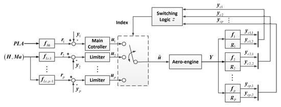
Figure 3.
Output-based multi-loop switching control strategy.
In Figure 3, the safety margin module implements mapping , and the parameter prediction module implements mapping , where . The images of key parameter under mapping and mapping are and , respectively, and these two parameters constitute the switching logic signal , namely:
The safety margin module and the parameter prediction module are described separately, and the specific design methods are given in the following sub-sections. Based on the design method of the above modules, the mechanism of the proposed output-based multi-loop switching control strategy was analyzed.
2.2.1. Safety Margin Module
It is assumed that the key engine parameter, , can be obtained directly, which includes the engine output parameter, , and the engine output parameter change rate, . In order to distinguish the upper-limited outputs from the lower-limited outputs, the safety margin module for output is described as follows:
where Equations (2) and (3) consider the upper and lower limited output respectively, and is defined as a warning factor to describe the distance between the safety margin and the given limit for the corresponding output.
2.2.2. Parameter Prediction Module
In order to realize mapping , the parameter prediction module for output, , is defined as follows:
where represents the system sampling time, and represents the prediction step size. Based on the current engine output change rates, these modules predict whether the engine will exceed the limit within a given prediction step size.
Finally, for the upper-limited outputs and the lower-limited outputs, based on Equation (1), the switching logic signal, , can be obtained by combining the results calculated by Equations (2) and (4), or Equations (3) and (5), respectively.
2.2.3. Switching Logic
After obtaining switching signal, , by exploiting the safety margin module and parameter prediction module, the switching logic needs to be designed to obtain the index value of the activated control loop. The mapping , realized by switching logic, is designed as follows:
It can be seen that the limiter, , is activated when the index equals . There must be one of the following two conditions holding: one is that the corresponding switching signal is greater than 0 for the upper-limited output; the other is that the corresponding switching signal is less than 0 for the lower-limited output when the limiter, , is activated. When none of the limiters have to be used, the index equaling to 1 means that the main controller is activated.
2.2.4. Mechanism Analysis of Output-Based Limit Management Method
The switching logic, Equation (6), establishes the connection between the sign symbol of the switching logic signal, , and the controller activation index. For the activation condition of the limiter, the following inequalities can be obtained by rewriting Equations (2)–(5).
Equations (7) and (8) are the conditions to be satisfied for the upper-limited output and the lower-limited output limiter to be activated, respectively. Taking the limiter activation condition in Equation (7) as an example, if the change rate of the current limit output is considered as the change rate at future time, the two inequalities hold at the same time, which means that the limit output has exceeded the safety margin described by the warning factor, and the limit output will exceed its limit value after sampling steps.
In order to describe the switching logic more vividly, Figure 4 gives a schematic diagram of the switching logic for the upper-limited outputs. In Figure 4, the abscissa axis represents time; ordinate axis represents specified output ; ordinates and represent the limit boundary—defined by safety margin—and the limit value, respectively; the black curve represents the response of system output , and and are the points on the output response curve at and . The tangent lines of point and point are shown in the green solid line. The slopes of the two tangents are the change rate, , of the output, , at the corresponding time. In order to obtain the system output predicted value after the predicted step , blue dotted lines— and —are made, respectively, and intersect the tangent lines of points and at the points and . It can be seen that for point , condition holds. However, the condition does not hold due to . Therefore, the limiter corresponding to the output will not be activated at . For point , both conditions and are satisfied; the controller will switch to the limiter corresponding to the output, .
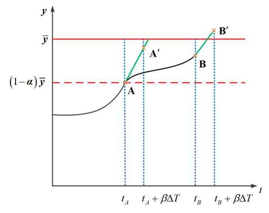
Figure 4.
Upper-limited output switching logic diagram.
Now the switching logic described above is directly applied to the multi-loop control of aero-engines to realize limit management. The control effect is shown in Figure 5. The controller index equal to 1 indicates that the main controller works; 2 indicates that the limiter corresponding to the total pressure at the outlet of the high-pressure compressor is activated, and 3 indicates that the limiter corresponding to the total temperature at the inlet of the mixing chamber is activated.
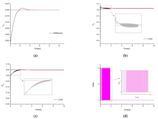
Figure 5.
Aero-engine response curves using direct switching method based on output-based switching logic: (a) High-pressure rotor corrected speed response; (b) High-pressure compressor outlet total pressure response; (c) Mixing chamber inlet total temperature response; (d) Controller index.
It can be seen that the multi-loop control method based on the non-linear output-based switching logic will lead to excessive overshoot and oscillation, which will seriously affect the control performance of the engine, although the high-pressure rotor speed finally tracks its reference. The reason for the problems above is that the difference of the engine control input signals before and after switching is too large. To solve the problem, the next section will introduce a bumpless transfer compensator based on the linear-quadratic index to govern the reference of the control loop so as to avoid large oscillations between the references and the control variables before and after controller switching, and to prevent the deterioration of control performance caused by integral saturation.
3. Realization Principle of Bumpless Transfer Method
In order to solve the aforementioned problems, a bumpless transfer scheme is proposed. As shown in Figure 6, the control objectives are as follows: (1) the on-line and off-line controllers can generate control input signals as close as possible; (2) the virtual references of the off-line controllers—obtained by the bumpless transfer compensator and the corresponding actual references—are as close as possible. The purpose of the former is to reduce the discontinuity of the engine control input before and after controller switching so as to avoid large oscillation in system responses and also to prevent the integral saturation of the off-line controller. The purpose of the latter is to maintain the tracking ability of the off-line controller and avoid the large difference between the actual and virtual references when the off-line controller is activated, which results in a large overshoot in the system response.
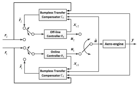
Figure 6.
Schematic diagram of bumpless transfer method.
Therefore, we need to find the gain of the bumpless transfer compensator, , in each control loop, which possesses the capacity of driving the corresponding off-line controller to generate control input signals similar to that generated by the on-line controller. Based on optimal control theory, the control objective of off-line controller’s () bumpless transfer compensator, , is expressed in a quadratic cost function as follows:
where , . , and are the control input signal of the aero-engine and reference signal of the on-line controller, respectively, and is the virtual reference signal that drives the off-line controller. and are positive definite matrices with appropriate dimensions. At the terminal time, , is the difference between the control inputs generated by the off-line controller and the online controller, and is the positive definite matrix. In order to obtain the gain of the bumpless transfer compensator, it is necessary to solve the optimization problem of minimizing Equation (9).
In order to obtain the gain, , the introduction of a linear state feedback controller was considered for the implementation of the control task. The structure of the off-line controller, , is as follows:
where is the ith controller state, , , , , and are constant matrices with appropriate dimensions. Since Equation (10) is a constraint for solving the cost function (9) minimization problem, it is necessary to construct a generalized function by introducing dynamic Lagrange multiplier .
where , the Hamilton functions can be defined as:
The necessary conditions for the minimization of Equation (9) are as follows:
Based on Equation (15), can be yielded as:
where .
Substituting Equation (16) into Equations (13) and (14), respectively, and organizing the acquired equations into a state-space form, the results are as follows:
where,
The non-homogeneous differential equation above is a common form of the linear-quadratic minimization problem, which can be solved by Sweep method [27]. According to [27], it can be assumed that can be expressed as follows:
The differential equation for Equation (20) is thus derived as:
By substituting Equations (21) and (22) into Equation (17), respectively, two different forms of differential equations about can be derived. By using the undetermined coefficient method, if we set the coefficients of the state of the off-line controller, , to be equal in two equations, we can obtain:
Considering the terminal time , Equation (23) degenerates from the differential Riccati equation to the algebraic Riccati equation:
The semi-positive definite matrix, , is the solution to the algebraic Riccati equation, Equation (24). At the same time, if we set the coefficients of other terms equal, we can obtain:
where,
Considering the terminal time , Equation (25) can degenerate into an algebraic equation:
where
The expression of in an infinite time domain can be obtained by substituting Equation (27) into Equation (16):
where,
Equation (29) can be rewritten as the following form:
where .
4. Design of Output-Based Aero-Engine Limit Management Method and Simulation Verification
4.1. Design of the Control Scheme for Aero-Engine Limit Management
Figure 7 presents a schematic diagram of the output-based bumpless transfer limit management method for aero-engines. In this figure, each controller works with a bumpless transfer compensator. The bumpless transfer compensator obtains the virtual reference, , by utilizing the controller state (), engine output (), engine control input (), and the corresponding reference (). The selection of the engine control input and the controller references (actual references or virtual references) depends on the index value given by the switching logic. As described in Section 2, the switching logic maps from the switching logic signal, , to the controller activation index, the safety margin module, and the parameter prediction module jointly realize the mapping from the key engine parameter, , to the switching logic signal, . Suppose that the controller activation index is , the controller is activated, the controller instruction is , and the engine control input equals . At this time, the virtual references, (for all ), obtained by the bumpless transfer compensator are used to ensure that the virtual reference, , and the actual reference, , as well as the value of the controller output, , and the engine control input, , are similar. When the controller activation index is switched from to , the bumpless transfer can be realized. Because of this property of the approach to bumpless transfer, if the control loop contains integral actions, the integral saturation caused by continuous integration of the off-line controller’s input can be avoided. Finally, the aero-engine output-based limit management control is realized by utilizing the structure shown in Figure 7.
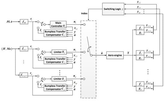
Figure 7.
Schematic diagram of the output-based bumpless transfer limit management method for the aero-engines.
4.2. Structural Transformation of the State Feedback Controllers
Consider the aero-engine state-space model:
where, for all , is the state, is the control input, is the output, and , , , and are appropriate dimensional constant matrices.
In order to incorporate the benefits of integral control action into the control method formulation, a state augmentation based on Equation (32) is utilized by introducing the control input, , into the system state:
where,
A state feedback controller, , to perform the tracking task of the system output, , to the reference, ri, is introduced as follows:
where , and , and can be calculated by the following equation according to the tracking task:
where and are the ith row vector of the system matrixes, and , respectively. Solve the Equation (36), and we can obtain:
Based on Equation (32), then:
By substituting Equations (37) and (38) into Equation (35), a new form of the state feedback controller can be obtained:
Let , then:
By integrating Equation (40) and assuming , the control law with an integral control action can be obtained:
It can be seen that the controller with integral control needs to be transformed into the form of Equation (10), then the controller can be applied to the design of the bumpless transfer compensator. By rewriting Equation (41) into the form of Equation (10), the following corresponding relations are obtained:
where, is the system output selection matrix, the element of the ith column is −1, and the elements of other columns are all 0. is the state variable selection matrix with appropriate dimensions. Its function is to extract the system state variables from the system outputs, which can be expressed as:
4.3. Aero-Engine Control Strategy for the Full Flight Envelope
4.3.1. Aero-Engine Linear Parameter Varying (LPV) Model
In order to verify the proposed method in the whole flight envelope, it is necessary to build an aero-engine LPV model. The LPV model has the ability to simulate engine dynamics behavior from idle to full power in the whole flight envelope and is defined by linear systems with the steady-state equilibrium point model (SSEPM) and the state variable model (SVM) sets. These models are affine functions of system operating parameters. The system dynamics are simplified and depicted as a single model by the LPV technique [34].
In the LPV framework, the engine model in Equation (32) can be written as follows:
where , , , and are functions of the engine operating parameters, , and can be obtained by the interpolation or fitting method. At each equilibrium point, the SVM can be obtained by using the hybrid fitting method [35].
Define as the deviation of the engine actual value from the corresponding equilibrium point value , namely:
where are the images of the mapping realized by the SSEPM.
We utilize the corrected low-pressure rotor speed increment, , and the corrected high-pressure rotor speed increment, , as states, and the corrected fuel flow increment, , as control input. We define output , where is the corrected total pressure increment of the high-pressure compressor outlet and is the corrected total temperature increment of the mixing chamber inlet. Equation (44) can thus be rewritten as:
Consider taking a steady-state equilibrium point every 2% of the corrected fuel value, , in the range from 0.21 to 1.04. At each equilibrium point, the SSEPM of the engine in the ground state is established. Finally, an SSEPM with 42 equilibrium points is constructed. The polynomial fitting method [36] is used to obtain the functional relationship between the system matrix coefficients and the operating parameters. Consider that the fitting accuracy of the polynomial fitting method increases with the increase of fitting order, but too high order will increase the calculation time when calling the model. Therefore, a tradeoff between calculation time and fitting accuracy should be considered. On the premise of keeping the order invariant, segmenting the model is a method to improve the fitting accuracy of the model.
Now the corrected high-pressure rotor speed, , is used as the abscissa; the matrix element value is used as the ordinate; and equals 0.935 as the segmented point. Then an aero-engine LPV model can be built (see Appendix A) and the relationship between the engine operating parameter, , and the matrix elements of the LPV model in Equation (46) is depicted from Figure 8, Figure 9, Figure 10 and Figure 11.
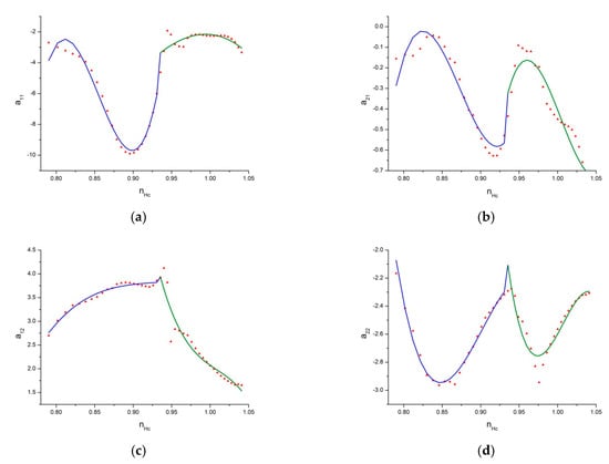
Figure 8.
Matrix elements in the system matrix : (a) ; (b) ; (c) ; (d) .
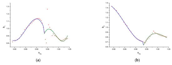
Figure 9.
Matrix elements in the system matrix : (a) ; (b) .
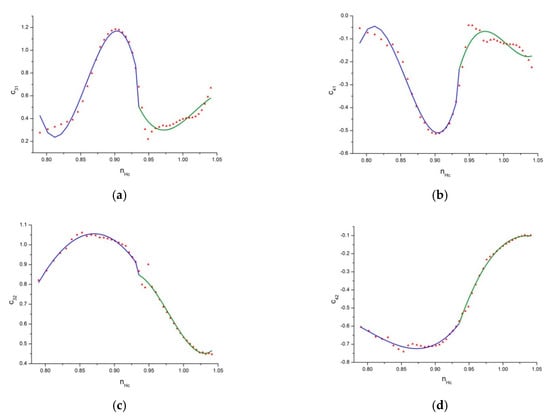
Figure 10.
Matrix elements in the system matrix : (a) ; (b) ; (c) ; (d) .
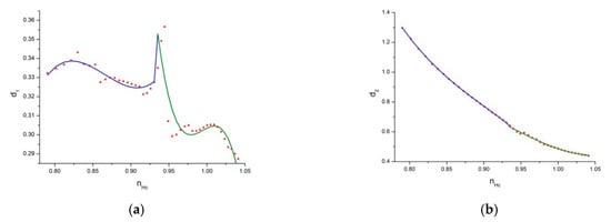
Figure 11.
Matrix elements in the system matrix : (a) ; (b) .
The SSEPM is constructed by using the interpolation method, and is depicted by the following Figure 12:
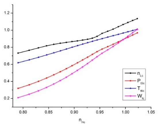
Figure 12.
Schematic diagram of the relationship between the operating parameter and the steady-state parameters of the aero-engine.
4.3.2. Control Plan Implementation Method Based on the Similarity Principle
After establishing the LPV model, a control method suitable for a wide range of engine models should be considered to be adopted. Envelope partition and similarity principle are the two methods to realize the whole envelope control of the engine. In this paper, the latter method was chosen. When the gain scheduling method is used to realize the limit management control of the aero-engine within the full flight envelope, the engine control plan must be taken into account to obtain a more practical control scheme.
Generally, the control plan of the aero-engine includes the low-pressure rotor speed control plan, the high-pressure rotor speed control plan, the mixing chamber inlet total temperature control plan, and the high-pressure compressor outlet total pressure control plan, i.e., , , , and . It can be seen that the control plan of each controlled parameter is a function of the flight condition because the inlet total temperature, , is a function of the flight condition. In order to distinguish from the main control plan , the four control plans above are called limit plan.
If the engine is operated under condition , then can be obtained by using the function [27]. Then, the values obtained by the limit plans as the limit parameters—i.e., , , , and —are exploited to acquire similar parameters under the ground condition by the similarity principle method:
where the subscript denotes the design points, and is used to distinguish from , which is the engine corrected high-pressure rotor speed reference obtained by PLA.
Then based on Equation (41), the control laws can be given by:
where , , , and are the controller gains for the limit plans and are obtained by the following interpolation map:
The optimal augmented monotonic tracking controller (OAMTC) method [9] was considered to be used for designing the controllers in this paper. Because the controlled parameters of the limit plan, , and the main control plan, , are both , the two plans adopt the same controller gain, . For , let two poles be placed at and . For , the poles are placed at and . For , the pole is placed at , and at for . It should be noted that the OAMTC method is essentially a pole placement method, and its control objective is to shape the controlled variable with monotonicity property and to ensure the stability of the closed-loop system. The value to be assigned is the pole of the closed-loop system, and it can be obtained by using genetic algorithm. For more details, see [9]. The map in Equation (49) can be described in Figure 13:
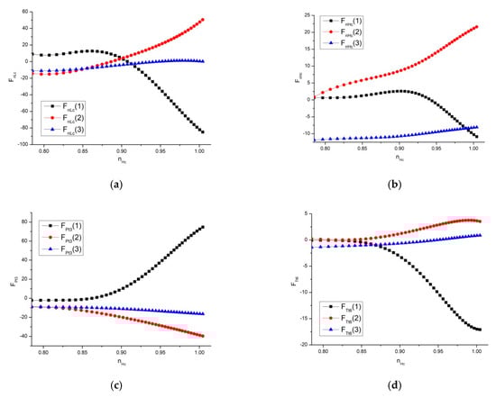
Figure 13.
The maps of the controller gains: (a) ; (b) ; (c) ; (d) .
4.4. Results and Discussion
This chapter includes two parts: one is the analysis of the influence of the warning factor, , and the predictive step size, , on the control performance; the other is the feasibility verification of the method proposed in this paper for the limit management control within the whole flight envelope. In this paper, numerical simulation work was carried out on the aero-engine nonlinear component-level model. The computer was configured as Intel Core I3 2.53 GHz with 2 G memory. The single calculation time of the controller was less than 5 ms, far less than the sampling period of 20 ms, which met the real-time requirement.
4.4.1. Analysis of the Parameter Characteristics
In order to improve the limit management ability, the parameters of safety margin module and parameter prediction module must be reasonably selected. To determine an acceptable value of for a specific limiter, it is necessary to “ignore” the parameter prediction module by setting to infinity in Equations (4) and (5). Then, only the safety margin module can be used to obtain the index of the limiter, which consists of two functions, Equations (2) and (3).
To simplify the analysis conditions, only the main control plan and limit plans for and were considered, and the parameters and , corresponding to the limit plan for , were set to a fixed value. Let ; then, only the influence of the different on the control performance was studied. Figure 14 shows the simulation results of the acceleration control of the engine operating from idle to full power under the ground condition with different , where the controller index being 1 indicates that the main controller is activated, 2 indicates the limiter for is activated, and 3 indicates the limiter for is activated.
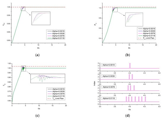
Figure 14.
Simulation results of the acceleration control with different : (a) Corrected high-pressure rotor speed response; (b) High-pressure compressor outlet total pressure response; (c) Mixing chamber inlet total temperature response; (d) Controller index.
From Figure 14, it can be seen that, with the increase of , the response of the high-pressure rotor speed and the high-pressure compressor total pressure became slower; the further the peak value of the mixing chamber total temperature response is away from the limit value, the more frequent the switches of the controller. However, too frequent switching lead to the unsatisfactory oscillation problem of the system responses. It can be understood that with the increase of , the farther the safety margin, , is from the limit value, , the easier to meet the conditions in Equation (7), and the less likely the limit violation occurs, so the number of the limiter activation increases, as shown in Figure 14d. In order to make a trade-off between the safety and the number of the controller switching, is decided to be set at 0.0078.
Then the influence of different parameter, , on the control performance was studied based on . Figure 15 shows the simulation results of the acceleration control of the engine with different .
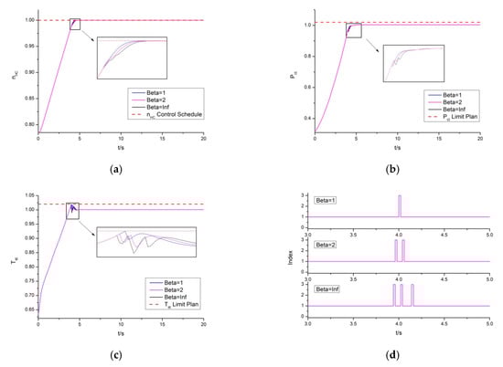
Figure 15.
Simulation results of the acceleration control with different : (a) Corrected high-pressure rotor speed response; (b) High-pressure compressor outlet total pressure response; (c) Mixing chamber inlet total temperature response; (d) Controller index.
From Figure 15, it can be seen that with the increase of , the lower the response speed of the high-pressure rotor speed and the high-pressure compressor outlet total pressure becomes, the farther the peak value of the mixing chamber inlet total temperature response deviates from the limit value, and the number of controller switching increases. It can be understood that, based on the current output change rate, if the output response moves towards its limit value, the more likely it will satisfy the activation condition with the value of being larger. In Figure 15b, the number of the controller switching increases with the increase of . It can be seen from Figure 15c that the limiter is activated when the corresponding output response is far away from its limit value, which limits the peak value of its response to be inaccessible to the limit boundary. Therefore, the response speed decreases with the increase of . Similarly, in order to obtain the fastest response, is decided to be set at 1.
4.4.2. Simulation Results and Discussion
The process of determining the parameters α and β in last sub-section is then repeated for each of the other engine limiters. In this subsection, the parameters are set as follows:
The design parameters of the bumpless transfer compensator are given by:
The gain of the bumpless transfer compensator in each control loop can be obtained by the following gain schedule method:
By using the output-based limit management control method proposed in this paper (OBC), the simulation operating from the idle to full power under the ground condition is shown in Figure 16, which is verified by comparing the control performance with the Min-Max scheme. The controller index of 1 indicates the main controller is activated; 2 indicates the limiter for is activated; 3 indicates the limiter for is activated; 4 indicates the limiter for is activated; and 5 indicates the limiter for is activated. Two kinds of controllers are chosen for building the multi-loop limit management structure based on the Min-Max scheme—the OAMTC controller and the LMI controller (LMIC) proposed in [10].
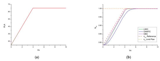
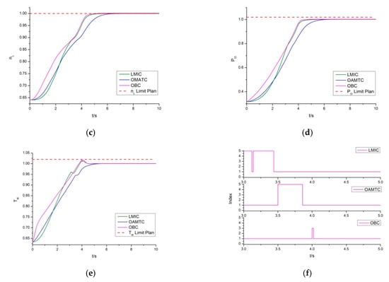
Figure 16.
Simulation results of the acceleration limit management control under the ground condition: (a) PLA; (b) Corrected high-pressure rotor speed response; (c) Low-pressure rotor speed response; (d) High-pressure compressor outlet total pressure response; (e) Mixing chamber inlet total temperature response; (f) Controller index.
In Figure 16b, it can be seen that the response speed of the OBC method is basically the same as that of the LMIC method, both of which have a faster response speed than that of the OAMTC method. From Figure 16b–e, it can be seen that all of the three limit management control methods (OAMTC, LMIC, and OBC) can realize the steady protection and transition limit protection of the engine, and there is no limit violation occurring. From Figure 16f, it can be seen that, for the LMIC and OAMTC methods based on the Min-Max scheme, the output limits are not exceeded before , but their corresponding limiters have been activated. The reason for that is the switching action of the controller is only related to the fuel change rate of each loop. However, for the OBC method, the switching action of the controller is determined by the output-based switching logic signal, and the problem above will be solved. From Figure 16f, it can be seen that has the possibility of exceeding its limit at . Then the main controller is switched to the limiter by the switching logic, which realizes the transition limit protection. It can be seen that the OBC method establishes a direct relationship between the switching action of the controller and the limit violation.
Finally, the simulation validation of the limit management control in the flight envelope is carried out operating at the full power condition, which is shown in Figure 17.
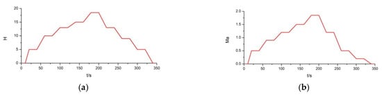
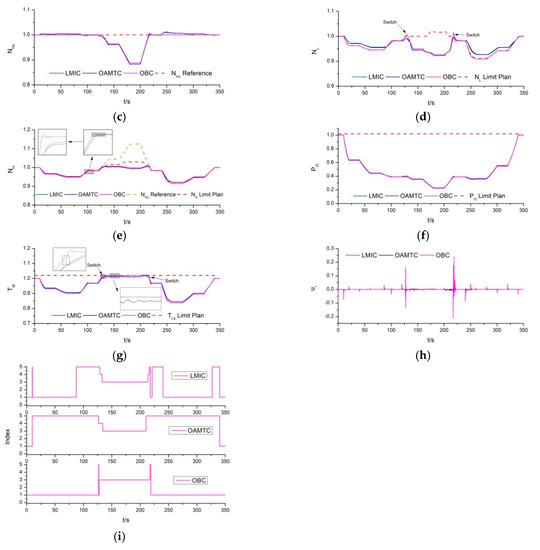
Figure 17.
Simulation results under full power condition within the whole flight envelope: (a) Altitude; (b) Mach number; (c) Corrected high-pressure rotor speed response; (d) Low-pressure rotor speed response; (e) High-pressure rotor speed response; (f) High-pressure compressor outlet total pressure response; (g) Mixing chamber inlet total temperature response; (h) Control Input; (i) Controller index.
The altitude and Mach number curves are shown in Figure 17a,b, respectively. In Figure 17c, the OAMTC and the LMIC response curves basically coincide. A significant difference between the control effect of these response curves and that of the OBC method is whether the steady-state tracking error exists or not. It can be seen that for OBC method, the response tracks its reference with no steady-state error and satisfactory dynamic performance. However, steady-state errors cannot be eliminated by the OAMTC and the LMIC method. The reason is that, for these two methods, the steady-state is used as the tracking reference which is obtained by the interpolation method, and the error between the actual steady-state of the engine corresponding to the tracking reference, , and the “interpolation” steady-state will be introduced. In Figure 17d, the OBC response keeps within the limit, whereas the responses of Min-Max based methods exceed the limit. Viewing that the Min-Max scheme is able to realize the steady limit protection, the limit violation may be caused by the “error” mentioned above. In Figure 17e–g, the limit protection for the limit plans of , , and are all realized, but the control performance of the OBC method is better than that of the other methods. And as shown in Figure 17i, the fewer number of controller switching events carried out by the OBC method proved that the proposed strategy established the relationship between the switching action and the limit violation and provided faster control performance. Therefore, the method presented in this paper has the potential for application in actual engine control systems.
5. Conclusions
This paper has proposed a new limit management control approach to ensure the operational safety of aero-engines. The novelty of this methodology lies in the multi-loop switching control strategy with the output-based switching logic. It consists of the following design points: the design of the safety margin module, the parameter predictive module, and the switching logic, and also the method to realize bumpless transfer. Compared with the Min-Max scheme, one advantage of this methodology is that the switching logic signal obtained by the safety margin module and the parameter predictive module establishes the connection between the switching action and the limit violation, and, therefore, the limit violation can be directly avoided. Another advantage of this methodology lies in the subsequent reduction of the controller switching frequency, which improves the control performance. From the results of simulations varying from acceleration control to steady control scenarios, conclusion can be drawn that the proposed strategy has superiority over the Min-Max strategy in transient limit protection and has the potential for application in the aero-engine control practice.
Author Contributions
Conceptualization, J.Q.; Data curation, J.Q.; Formal analysis, J.Q. and J.H.; Funding acquisition, J.H.; Investigation, J.H.; Methodology, J.Q.; Project administration, J.H.; Resources, M.P.; Software, J.Q. and W.X.; Supervision, J.H.; Validation, J.Q. and W.X.; Visualization, J.Q.; Writing—original draft, J.Q.; Writing—review & editing, M.P. and J.H.
Funding
This research was funded by National Science and Technology Major Project of China, grant number [2017-V-0004-0054].
Conflicts of Interest
The authors declare no conflict of interest.
Appendix A
The LPV model matrix elements corresponding to Equation (46) are as follows:
(1)
(2)
References
- Spang, H.A.; Brown, H. Control of jet engines. Control Eng. Pract. 1999, 7, 1043–1059. [Google Scholar]
- Richter, H.; Litt, J.S. A novel controller for gas turbine engines with aggressive limit management. In Proceedings of the 47th AIAA/ASME/SAE/ASEE Joint Propulsion Conference & Exhibit, San Diego, CA, USA, 31 July–3 August 2011. [Google Scholar]
- Richter, H. Advanced Control of Turbofan Engines; Springer: New York, NY, USA, 2012; pp. 140–228. [Google Scholar]
- Sun, J.; Vasilyev, V.; Ilyasov, B. Advanced Multivariable Control Systems of Aeroengines; Beihang Press: Beijing, China, 2005; pp. 60–83. [Google Scholar]
- Burcham, F.W.; Fullerton, C.G.; Maine, T.A. Manual Manipulation of Engine Throttles for Emergency Flight Control; NASA Reports; NASA: Washington, DC, USA, 2004.
- Richter, H. Control design with output constraints: Multi-regular sliding mode approach with override logic. In Proceedings of the 2012 American Control Conference (ACC), Montreal, QC, Canada, 27–29 June 2012. [Google Scholar]
- Richter, H. Multiple sliding modes with override logic: Limit management in aircraft engine controls. J. Guid. Control Dyn. 2012, 35, 1132–1142. [Google Scholar] [CrossRef]
- Du, X.; Richter, H.; Guo, Y. Multivariable Sliding-Mode Strategy with Output Constraints for Aero-engine Propulsion Control. J. Guid. Control Dyn. 2016, 39, 1631–1642. [Google Scholar] [CrossRef]
- Yu, B.; Ke, H.; Shu, W. A Novel Control Scheme for Aircraft Engine Based on Sliding Mode Control with Acceleration/Deceleration Limiter. IEEE Access 2019, 7, 3572–3580. [Google Scholar] [CrossRef]
- Yang, S.; Wang, X.; Yang, B. Adaptive sliding mode control for limit protection of aircraft engines. Chin. J. Aeronaut. 2018, 148, 78–86. [Google Scholar] [CrossRef]
- Qin, J.; Huang, J.; Pan, M. Optimal augmented monotonic tracking controller for aircraft engines with output constraints. Energies 2017, 10, 73. [Google Scholar] [CrossRef]
- Imani, A.; Montazeri-Gh, M. Improvement of Min-Max Limit Protection in Aircraft Engine Control: An LMI Approach. Aerosp. Sci. Technol. 2017, 68, 214–222. [Google Scholar] [CrossRef]
- Qin, J.; Pan, M.; Huang, J. A multi-regulator linear matrix inequalities approach for aircraft engines limit management. Int. J. Turbo Jet-Engines 2018. [Google Scholar] [CrossRef]
- May, R.D.; Garg, S. Reducing conservatism in aircraft engine response using conditionally active min-max limit regulators. In Proceedings of the ASME Turbo Expo: Turbine Technical Conference and Exposition, Copenhagen, Denmark, 11–15 June 2012. [Google Scholar]
- Richter, H. A multi-regulator sliding mode control strategy for output-constrained systems. Automatica 2011, 47, 2251–2259. [Google Scholar] [CrossRef]
- Imani, A.; Montazeri-Gh, M. A Multi-loop Switching Controller for Aircraft Gas Turbine Engine with Stability Proof. Int. J. Control Autom. Syst. 2019, 17, 1359–1368. [Google Scholar] [CrossRef]
- Seok, J.; Kolmanovsky, I.; Girard, A. Coordinated Model Predictive Control of Aircraft Gas Turbine Engine and Power System. J. Guid. Control Dyn. 2017, 40, 1–18. [Google Scholar] [CrossRef]
- Richter, H.; Singaraju, A.V.; Litt, J.S. Multiplexed Predictive Control of a Large Commercial Turbofan Engine. J. Guid. Control Dyn. 2008, 31, 273–281. [Google Scholar] [CrossRef]
- Peng, K.; Fan, D.; Yang, F. Active generalized predictive control of turbine tip clearance for aero-engines. Chin. J. Aeronaut. 2013, 26, 1147–1155. [Google Scholar] [CrossRef]
- Xu, W.; Pan, M.; Qin, J.; Huang, J. Reference and limit governors for limit protection of turbofan engines. Energies 2019, 12, 2803. [Google Scholar] [CrossRef]
- Hui, Y.; Mou, C.; Wu, Q.X. Flight envelope protection control based on reference governor method in high angle of attack maneuver. Math. Probl. Eng 2015, 2015, 254975. [Google Scholar]
- Kalabic, U.V.; Buckland, J.H.; Cooper, S.L.; Wait, S.K.; Kolmanovsky, I.V. Reference governors for enforcing compressor surge constraints. IEEE Trans. Control Syst. Technol. 2016, 24, 1729–1739. [Google Scholar] [CrossRef]
- Garone, E.; Di Cairano, S.; Kolmanovsky, I. Reference and command governors for systems with constraints: A survey on theory and applications. Automatica 2017, 75, 306–328. [Google Scholar] [CrossRef]
- Day, I. Stall, Surge and 75 Years of Research. J. Turbomach. 2016, 138, 011001. [Google Scholar] [CrossRef]
- Campo, P.J.; Morari, M.; Nett, C.N. Multivariable anti-windup bumpless transfer schemes. In Proceedings of the American Control Conference, Pittsburgh, PA, USA, 21–23 June 1989. [Google Scholar]
- Edwards, C.; Postlethwaite, I. Anti-windup and bumpless transfer schemes. Automatica 1998, 34, 199–210. [Google Scholar] [CrossRef]
- Lewis, F.L. Optimal Control; Wiley International: New York, NY, USA, 1986. [Google Scholar]
- Green, M.; Limebeer, D.J.N. Linear Robust Control; Pearson Education: London, UK, 1995; pp. 415–448. [Google Scholar]
- Hanus, R.; Kinnaert, M.; Henrotte, J.L. Conditioning technique, a general anti-windup and bumpless transfer method. Automatica 1987, 23, 729–739. [Google Scholar] [CrossRef]
- Hyde, R.A. The Application of Robust Control to VSTOL Aircraft. Ph.D. Thesis, University of Cambridge, Cambridge, UK, 1991. [Google Scholar]
- Turner, M.C.; Walker, D.J. Linear-quadratic bumpless transfer. Automatica 2000, 36, 1089–1101. [Google Scholar] [CrossRef]
- Turner, M.C.; Aouf, N.; Bates, D.G.; Postlethwaite, I.; Boulet, B. Switched control of a vertical/short take-off land aircraft: An application of linear-quadratic bumpless transfer. Proc. Inst. Mech. Eng. Part I J. Syst. Control Eng. 2006, 220, 157–170. [Google Scholar] [CrossRef]
- Kowalski, K.K.; Achterberg, J.; Lierop, C.M.M.V. Implementation of a Linear Quadratic Bumpless Transfer Method to a Magnetically Levitated Planar Actuator with Moving Magnets. In Proceedings of the IEEE International Conference on Control Applications, Yokohama, Japan, 8–10 September 2010. [Google Scholar]
- Shamma, J.S. Analysis and Design of Gain Scheduled Control Systems. Ph.D. Thesis, Massachusetts Institute of Technology, Cambridge, MA, USA, 1988. [Google Scholar]
- Lu, F.; Qian, J.; Huang, J. In-flight adaptive modeling using polynomial LPV approach for turbofan engine dynamic behavior. Aerosp. Sci. Technol. 2017, 64, 223–236. [Google Scholar] [CrossRef]
- Zhou, W.X. Research on Object-Oriented Modeling and Simulation for Aero-Engine and Control System. Ph.D. Thesis, Nanjing University of Aeronautics and Astronautics, Nanjing, China, 2007. [Google Scholar]


© 2019 by the authors. Licensee MDPI, Basel, Switzerland. This article is an open access article distributed under the terms and conditions of the Creative Commons Attribution (CC BY) license (http://creativecommons.org/licenses/by/4.0/).