Development of the Availability Concept by Using Fuzzy Theory with AHP Correction, a Case Study: Bulldozers in the Open-Pit Lignite Mine

Abstract

Availability is one of the most used terms in maintainability engineering. This concept is used to denote: The quality of service of an engineering system, i.e., machines, weak points’ analysis, asset management, as well as making decisions in the process of life cycle management. Availability is an overall indicator and contains partial indicators that are oriented towards reliability, maintenance, and logistical support. Availability presents a variable value and changes in time and space. Usually, availability is shown as the coefficient of time use of the machine. This approach is not good enough because it does not go into the structure of the availability itself and requires a high level of IT support in system monitoring. In this sense, this paper will use the fuzzy theory and the corresponding analytic hierarchy process (AHP) multi-criteria analysis to present a conceptual and mathematical model for the assessment of availability based on expert judgment. The model will be shown in the case study (on the example) of bulldozers working in the open-pit lignite mine.

1. Introduction

Various explanations of the term availability are to be found in the literature. In essence, availability means the ability of the technical system to be able to perform the required function [1], under given conditions and at a specific moment in time, and assuming that the necessary supply is provided (external resources) [2]. Availability may also be expressed as the probability that the system will be ready for use at any (calendar) time, or that it will be in working order or ready to be activated [3]. System availability presents the degree of efficiency of the system in terms of getting started and achieving output values at the level of the allowed tolerances of the set function of the criteria in a given time and given surrounding conditions. Availability is determined depending on the function of flawless work, reliability and convenience of the maintenance function.

Functional safety is a common term used to describe availability and the factors that affect it: Reliability, convenience of maintenance, and maintenance support level. The term availability is used to denote the degree of functional safety. Availability is expressed in quantitative indicators, and as such, is a measure of functional safety, and thus of the quality of service. Monitoring and availability analysis are significant because of the known fact that the machine must, above all, be available for operation, in order to realize other operating performance. American military standard (MIL-STD) defines availability as a measure of the degree to which an item is in an operable state and can be committed at the start of a mission when the mission is called for at an unknown (random) point in time. Availability, as measured by the user, is a function of how often failures occur and corrective maintenance is required, how often preventative maintenance is performed, how quickly indicated failures can be isolated and repaired, how quickly preventive maintenance tasks can be performed, and how long logistics support delays contribute to downtime [4].

Achieving a satisfactory level of the machine availability in the use phase depends largely on appropriate maintenance procedures, logistical support, and the provision of appropriate means of maintenance. A variety of activities are involved in the attempt to reduce active and inactive maintenance time. The mentioned times are related to the maintenance work itself, as well as to the appropriate technical, logistical, and administrative waiting times. This requires appropriate efforts in planning and creating a realistic maintenance concept, a critical analysis of maintenance plans (maintenance levels, identification of needs, goals), defining requirements for logistics support tools (people, training, manuals, test, and auxiliary instruments, spare parts, etc.).

In the last decades of the 20th century, the concept of dependability management [5,6] was developed by the International Electro-Technical Commission (IEC) in order to provide an integrated approach to managing and ensuring: Safety management, availability, reliability, convenience of maintenance, and maintenance support system. This concept is also designated as an international standard IEC 300 [5], which, among other things, states that the performance of dependability includes availability as its measure [6]. Dependability is defined in [7] as “the ability to avoid service failures that are more frequent and more severe than is acceptable to the user”. In reference [8] dependability has been described as a tree that has three branches. The first branch includes the attributes that, in addition to availability, maintainability, and reliability, include: Safety, confidentiality, integrity. The second branch contains “means”, and it encompasses: Fault prevention, fault tolerance, fault removal, and fault forecasting. The third branch represents “threats”: Faults, errors, and failures. Although along the same lines, some authors have somewhat differently determined the interdependence between dependability and availability. In reference [8], dependability is defined as an indicator of “failure engineering”, which includes: Reliability, safety, convenience of maintenance, security, risk level, and quality. In reference [9], indicators such as maintenance time, maintenance work, maintenance frequency are added, along with active maintenance time, logistic delay time and administrative time, which define available time as an indicator of availability. In references [9,10], the authors give a literature overview, citing papers that mention efficiency and effectiveness as concepts close to availability and which are directly dependent on reliability. Generally, dependability as a measure of availability is only a standardized, all-in concept, which describes technical systems from the point of view of design, operation, and maintenance [11]. It is evident that the standard provides a descriptive and linguistic definition of dependability, without formal calculation, and consequently, availability as its measure remains mathematically and conceptually ambiguous. In references [12,13], it has been observed that the parameters defining quality of service are not consistent, but have considerable ambiguity, and cannot be expressed quantitatively, so the model of integration, based on the theory of fuzzy sets, has been developed. Theories of fuzzy logic are specifically used for description and proposition of indicators, i.e., their composition in which prevail uncertainty, indefinitely, multiplicity, subjectivity and mutual over-lapping. Fuzzy logic is used as a mathematical and conceptual model y expert systems with hybrid data. Unlike the classic crisp logic, fuzzy values are defined with membership function to proper linguistic variables [3]. The max–min composition was used, where the outcomes were defined as the mean value. In reference [14], the fuzzy theory was also used for the synthesis of available parameters, but reliability and the convenience of maintenance are presented on the basis of probability theory. Therefore, the concept of the fuzzification of the cumulative function has been introduced here. It can be concluded, on the basis of previous works, that a large number of partial indicators, which are overlapping between themselves, affect availability in many ways within technical systems, as well as within the same technical system at a different time (machine age) and spatial (work and service environment) coordinates. Partial indicators are reliability, convenience of maintenance from the construction point of view, convenience of maintaining from the logistical point of view, functionality and adaptability, safety (the level of risk to the work and environment).

Regardless of authors, it is evident that availability is essentially dependent on reliability, convenience of maintenance (structural component), and the level of support. Last mentioned item can be called supportability (S). The goals of supportability engineering are focused on minimizing the cost of ownership [15]. It contains a logistic component of maintainability and impact of the working environment in technical, functional, legal, administrative, financial, and any other ways [16]. These partial availability indicators are of hybrid nature. Some can be expressed numerically, in the form of a time-dependent function, and some only on the basis of expert judgment. Among these indicators, uncertainty, subjectivity, versatility, inconsistency, and mutual overlap prevail. In scientific literature, fuzzy logic is usually applied to solve such conceptual problems [17].

In this paper, an alternative model for determining availability will be displayed, using expert judgment, fuzzy inference, and the analytic hierarchy process (AHP) ranking method. The model contains structural decomposition of availability as an indicator quality of service of the engineering system, their independent analysis, and ranking, and finally gives the possibility of composition. Structural definitions of each outcome are given in accordance with the work environment. The result has two dimensions, one is the linguistic description of availability and the other is the intensity of the same. The model can be used as a simple tool in asset management in the sense of machine comparison and weak point analysis [18]. The model will be illustrated with the example of auxiliary machinery working in EPS (Electric Power Industry of Serbia) mines. The model will be verified by using the common ways to determine availability.

2. Materials and Methods

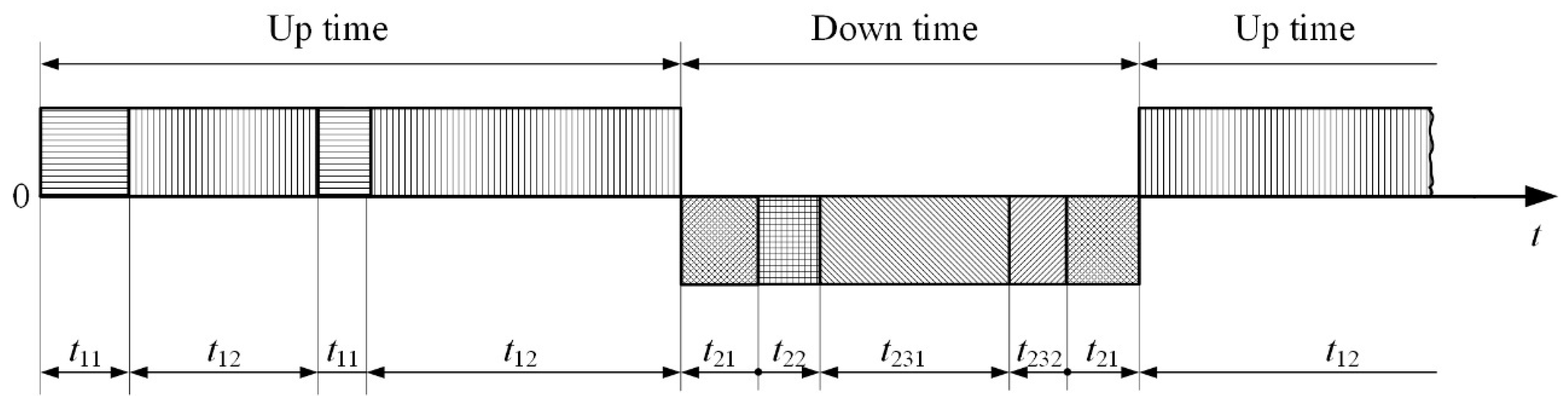
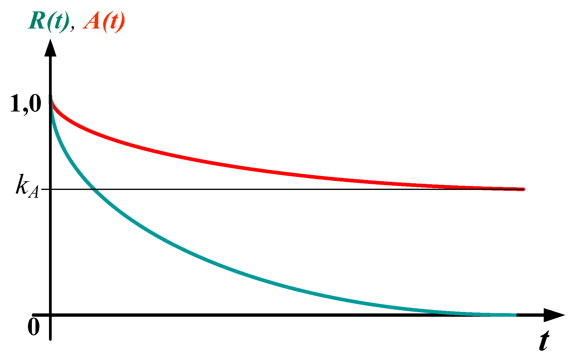
2.1. The Availability Concept in the Technical Systems of Maintenance Engineering

Availability is calculated on the basis of the time state picture, in which times of operation alternate with times of failure. The time state picture, i.e., the time and maintenance time structure for analyzing the availability of technical systems is shown in Figure 1, where, in general, t₁ is uptime, and t₂ is downtime. The time when the system is in its proper state can be divided into inactive time or the standby time (t₁₁) and the time when the system is in operation (t₁₂). The time of failure is divided into: organizational time (t₂₁), logistical time (t₂₂) and active repair time (t₂₃), which can be time for corrective repairs (t₂₃₁) and time for preventive repairs (t₂₃₂). The times t₂₁ and t₂₂ refer to: Defects, design interventions, administrative work, spare parts, tools, skilled labor, etc. The active repair time includes repair, assembly, disassembly, replacement, etc. The timetable is not always the same type. Figure 1 is just one of the possible examples.

Availability is determined by the total cumulative amount of time during which the system is in the correct state and the total time in work, including operational and failure states, or as:

$$A(t)=\frac{{\displaystyle \sum t_{11},t_{12}}}{{\displaystyle \sum t_{11},t_{12}},t_{21},t_{22},t_{231},t_{232}}$$

(1)

The above representation is often referred to as operation availability and is designated as A_o(t). If, when determining the availability in time of failure, only the active time of corrective and preventive maintenance is taken into account, we are referring to achieved availability:

$$A_a(t)=\frac{{\displaystyle \sum t_{11},t_{12}}}{{\displaystyle \sum t_{11},t_{12}},t_{231},t_{232}}$$

(2)

Inherent availability is obtained when only active corrective maintenance time is taken into account:

$$A_i(t)=\frac{{\displaystyle \sum t_{11},t_{12}}}{{\displaystyle \sum t_{11},t_{12}},t_{231}}$$

(3)

In a smaller number of cases, an accurate form for the availability function can be obtained. Availability can be displayed based on mean time between maintenance MTBF and mean downtime MDT.

$$A=\frac{MTBF}{MTBF+MDT}$$

(4)

For example, for the exponential function of reliability R(t) = e^–λ·t and convenience of maintenance M(t) = 1 − e^{−μ t}, it is known as:

• failure intensity: $\lambda =\frac{1}{MTBF}=const.$
• maintenance intensity: $\mu =\frac{1}{MDT}=const.$

The availability function A(t) in this case can be obtained as:

$$A(t)=\frac{\mu }{\lambda +\mu }+\frac{\lambda }{\lambda +\mu }\cdot e^{-(\lambda +\mu )\cdot t}$$

(5)

where the stationary value of the availability can be obtained as:

$$A=k_A=\underset{t\to \infty }{\lim }A(t)=\frac{\mu }{\lambda +\mu }=\frac{1}{1+\frac{\lambda }{\mu }}$$

(6)

The k_A value is called the coefficient of availability and is obtained when A(t) is calculated for t→ ∞, or when the availability value becomes stationary (Figure 2).

Figure 2 shows the relationship between availability and reliability. It is obvious that the availability requirement is much more stringent than the requirement of reliability, R(t) ≤ A(t).

In real conditions of the exploitation and maintenance of technical systems, availability is shown appropriately Equations (1)–(3), depending on the data recorded. The conditions are rarely met to analytically determine the availability function in the form of Equations (4) and (5). To determine availability in this way, an appropriate IT structure for keeping track of time t_i is required. In real terms related to complex machine engineering systems, this condition is usually not fulfilled or only partially fulfilled. Another problem is that we cannot infer the availability structure by knowing the availability coefficient. In other words, we do not know the impact of partial indicators such as reliability, the convenience of maintenance, and the level of support.

2.2. Expert Fuzzy-AHP Synthesis Model Availability

The expert model consists of two modes of expertise. One mode is represented by a questionnaire, which is filled in based on linguistic descriptions for each partial availability indicator. The linguistic descriptions are predefined. The expert records them with the membership function in the interval of 0…1. The questionnaires are statistically processed and translated into a fuzzy form. The second mode of the expert assessment is represented by the mutual ranking of partial indicators. In this paper, ranking is done using the AHP method.

The Fuzzy-AHP synthesis model is represented through the fuzzy inference model where inputs are represented with fuzzificated estimates of partial indicators, and the rules of fuzzy composition are defined through outcomes that are corrected on the basis of ranks.

2.2.1. Fuzzy Inference in the Synthesis Model

Availability (hereinafter referred to as A) is defined as a comprehensive (umbrella) term, which contains the following phenomena: reliability (R), maintainability (M), supportability (S) [19].

The first step in the formation of the synthesis model is the availability proposition and its partial indicators (R, M, S). Five linguistic variables are introduced for each indicator, which are defined in the coordinate system of the membership function (μ), and the class as the representative of the unit of indicator measure (j) [20]. The linguistic variable (LV) is generally defined as follows:

$$LV=\left({\mu }_{(j=1)},\dots ,{\mu }_{(j=10)}\right)$$

(7)

Each linguistic variable (‘A’, …,‘E’) is specifically defined in the following way (Figure 3):

$$\begin{array}{l}\prime \mathrm{A}\prime =(0_{(1)},\dots .,0_{(8)},1_{(9)},1_{(10)});\\ \prime \mathrm{B}\prime =(0_{(1)},\dots .,0_{(5)},{0.33}_{(6)},1_{(7)},1_{(8)},0_{(9)},0_{(10)});\\ \prime \mathrm{C}\prime =(0_{(1)},0_{(2)},0_{(3)},{0.5}_{(4)},1_{(5)},1_{(6)},{0.5}_{(7)},0_{(8)},0_{(9)},0_{(10)});\\ \prime \mathrm{D}\prime =(0_{(1)},0_{(2)},1_{(3)},1_{(4)},{0.33}_{(5)},0_{(6)},\dots ,0_{(10)});\\ \prime \mathrm{E}\prime =(1_{(1)},1_{(2)},0_{(3)},\dots ,0_{(10)}).\end{array}$$

For each partial indicator, a description of each linguistic variable is defined. The following descriptions are given below:

Reliability:

• ‘A‘(R)—No sudden, unplanned failures were recorded.
• ‘B‘(R)—There are some interruptions in work. Negligible impact on the time state picture of the technical system.
• ‘C’(R)—Failures occur. In most cases, they are expected, and therefore, in some way they can be planned. Failures can be eliminated on the spot.
• ‘D’(R)—Occurrence of failure is frequent. The reliability of the machine is low. Efficiency is reduced.
• ‘E’(R)—Constant breakdowns occur. The machine is not at the required working level.

Maintainability:

• ‘A’(M)—Any intervention can be fully planned in terms of time and work organization. Diagnosis is simple. Repairs are quick. No corrosion. Defective parts are not of a large mass. It is possible to plan time and work organization.
• ‘B’(M)—Quick identification of weaknesses is possible (errors, faults …). It is constructively easy to repair. There may be some minor interference errors.
• ‘C’(M)—Possible difficulties during preventive and service maintenance, for reasons of constructive nature, inaccessibility of parts, due to the appearance of corrosion, the mass of the element, and the like.
• ‘D’(M)—It is not possible to plan the duration of the intervention and the organization of work. There are a number of complications during dismantling and assembly.
• ‘E’(M)—The breakdown cannot be remedied in an acceptable time. It is necessary to disconnect the machine from the operating unit for a longer period of time.

Supportability:

• ‘A’(S)—Any work with the machine can be fully planned in terms of time and organization. There are spare parts and tools. There are trained repairmen. The workshop is close. There are no administrative difficulties.
• ‘B’(S)—Administrative and logistical support is at a satisfactory level. Supply of spare parts is fast. Workshop is at a short distance. Possible purchase of necessary paperwork.
• ‘C’(S)—All activities related to maintenance support (spare parts, tools, workshops, employee training, etc.) are at a satisfactory level. Utilization of the machine is correct in most cases.
• ‘D’(S)—There are difficulties in purchasing spare parts. Additional training is necessary. There are administrative difficulties. Utilization of the machine is a little bit harder than expected.
• ‘E’(S)—There are no spare parts. The workers are not trained. There are administrative problems. The workshop is remote. Every utilization of the machine is full of unpredictability due to inadequate training, logistical support, etc. It is not possible to plan activities in the context of time and organization.

The second step in the formation of the synthesis model is the composition of partial parameters to the synthesis level. Basically, the composition in the fuzzy theory is represented by the ‘IF-THEN’ rule. In concrete cases, derived models of composition are used. In the literature [10,11,12,13,14], two models of composition are most often mentioned. Max–min composition, also called a pessimistic composition due to the process by which it is performed. A synthesis assessment is obtained by using a representative partial assessment that is defined as the best possible among the worst expected individual assessments. This composition is used to represent a phenomenon such as safety or dependability. Min–max composition is a model of fuzzy composition that is declared as an optimistic composition, because through it, the synthesis assessment is represented by a partial estimate that is the worst among the best expected partial assessments and is used, for example, to represent risk priority number. Below, a fuzzy min–max model of the composition is shown (steps i–vii).

$$A_i=\max \left\{\min (R_i,M_i,S_i)\right\}$$

(8)

(i) Three fuzzy numbers R_i, M_i и S_i are defined through membership function μ and class j = 1 to n:

$$\begin{array}{l}{R}_i=({\mu }_{R(1)},\dots ,{\mu }_{R(j)},\dots ,{\mu }_{R(n)});\\ M_i=({\mu }_{M(1)},\dots ,{\mu }_{M(j)},\dots ,{\mu }_{M(n)});\\ S_i=({\mu }_{S(1)},\dots ,{\mu }_{S(j)},\dots ,{\mu }_{S(n)}).\end{array}$$

(9)

(ii) The membership functions can form C = n³ combinations among themselves. Each combination A_c represents practically one possible assessment A_i(8).

$$A_c=\left[{\mu }_{R(j=1,\dots ,n)},{\mu }_{M(j=1,\dots ,n)},{\mu }_{S(j=1,\dots ,n)}\right],$$

(10)

for each c = 1 to C.

(iii) If only values that satisfy the condition μ_{R,M,S (j = 1,…, n)} ≠ 0, are taken into account, then we obtain the outcomes (o = 1 to O, where O ≤ C). Each outcome has the corresponding values (iv) and (v) that further identify it for the estimate.

(iv) Below, for each combination c that satisfies the condition of the outcome, the J_c value is calculated and rounded as an integer, in the following way:

$$J_c=\left[\left(w_{Ri}\cdot j_{(\mu R)c}\right)+\left(w_{Mi}\cdot j_{(\mu M)c}\right)+\left(w_{Si}\cdot j_{(\mu S)c}\right)\right]$$

(11)

wherein:

• w_i is the influential factor of the corresponding partial indicator on availability obtained on the basis of mutual ranking of partial indicators, where w_Ri + w_Mi + w_Si = 1 (Equation (17));
• j_c is a class to which the corresponding fuzzy number (9) belongs for the observed membership function and the given combination c, where j_c = 1, …, n;

(v) For each output, the minimum value μ_R, μ_M, μ_S in the vector A_c(10) is requested as follows:

$$M{N}_o=\min \left\{{\mu }_{R(j)o},{\mu }_{M(j)o},{\mu }_{S(j)o}\right\},$$

(12)

for each o = 1 to O

(vi) The outcomes are grouped according to J_c value. The number of such groups can be 0 to n.

(vii) In each outcome group (vi), the maximum MX value is requested among the identified minima (v). The maximum that corresponds to jth values is calculated as:

$$M{X}_j=\max {\left\{M{N}_1,\dots ,M{N}_0,\dots ,M{N}_O\right\}}_{J_c},$$

(13)

for each j = 0.

The assessment of the availability of the observed engineering system is finally obtained in a form that agrees with its Equations with (7) and (8):

$$A=\left(M{X}_{j=1},\dots ,M{X}_{j=n}\right)=\left({\mu }_{A(1)},\dots ,{\mu }_{A(j)},\dots ,{\mu }_{A(n)}\right)$$

(14)

The Equation (14) gives an assessment depending on the membership function and the class. Using some of the identification methods, the equation could be expressed depending on the linguistic variables ‘A’, ‘B’, ‘C’, ‘D’, and ‘E’, in accordance with Figure 3. In this paper, the best-fit method will be used. This method is special in that it allows the possibility of mapping the membership function to classes (14) in the membership function of the fuzzy numbers (15), respectively mapping the membership function into a given final value in the membership function to a given surface. The model is based on the calculation of the relative distance between the given final value of the membership function of the obtained result and the membership function of the fuzzy number that defines the linguistic variables ‘A’, …, ‘E’. A detailed presentation will be given in the case study.

$$A={\mu }_{\prime \mathrm{A}\prime }/\prime \mathrm{A}\prime ,{\mu }_{\prime \mathrm{A}\prime }/\prime \mathrm{B}\prime ,{\mu }_{\prime \mathrm{A}\prime }/\prime \mathrm{C}\prime ,{\mu }_{\prime \mathrm{A}\prime }/\prime \mathrm{D}\prime ,{\mu }_{\prime \mathrm{A}\prime }/\prime \mathrm{E}\prime$$

(15)

2.2.2. AHP Ranking Model

The analytical hierarchical process (AHP) represents the most commonly used mathematical method in multi-criteria decision making (MCDM). Designed by Saaty [21], from its very appearance, the method has attracted great interest, and today methods of this type are widely used and have broad application.

It relies on the theory of relative measurements of the severity of the impact factors in decision making. The subject of interest is not the accurate measurements of individual quantities, but the accent is placed on a proportional relationship between them [22]. It is based on the measurement comparing pairs, depending on the expert assessment in defining the priority scales [23]. One of the advantages of the AHP method is its ability to identify and analyze the inconsistency of the decision-maker in the process of prioritizing the hierarchical structure [24].

According to assumptions from human psychology, the simplest decisions can be made when there are only two alternative choices in one interaction. This is precisely the basic principle of the AHP method [22]. A complex problem is split into simple factors that are then compared in pairs. Each pair comparison is made using the Saaty scale of relative importance shown in

Table 1. Analytic hierarchy process (AHP) scale of importance.

The Level of Importance	Numerical Value	Reciprocal Value
Extreme importance	9	1/9 (0.111)
Very strong to extreme importance	8	1/8 (0.125)
Very strong importance	7	1/7 (0.143)
Strong to very strong importance	6	1/6 (0.167)
Strong importance	5	1/5 (0.200)
Moderate to strong importance	4	1/4 (0.250)
Moderate importance	3	1/3 (0.333)
Equal to moderate importance	2	1/2 (0.500)
Equal importance	1	1 (1.000)

[25].

The result of a pair-wise comparison of the elements is the numerical value that presents the priority vector (W). According to Equation (16), the priority vectors of each element are calculated, after which the possibility of forming the mathematical matrix M (17) is created, whose calculation provides the solution according to a particular criterion or sub-criterion.

$$W={\displaystyle \sum _{j=1}^n\frac{W_i}{W_j}=}{W}_i\left({\displaystyle \sum _{j=1}^n\frac{1}{W_j}}\right)i=1,\dots ,n$$

(16)

$$M=\left[\begin{array}{cccc}{w}_1/w_1& w_1/w_2& \dots & w_1/w_n\\ w_2/w_1& w_2/w_2& \dots & w_2/w_n\\ \dots & \dots & \dots & \dots \\ w_n/w_1& w_n/w_2& \dots & w_n/w_n\end{array}\right]=\left[\begin{array}{cccc}{a}_{11}& a_{12}& \dots & a_{1n}\\ a_{21}& a_{22}& \dots & a_{2n}\\ \dots & \dots & \dots & \dots \\ a_{n1}& a_{n2}& \dots & a_{nn}\end{array}\right]$$

(17)

The last step in the AHP method is to check the error, i.e., verification of the consistency of the decision-maker [26,27]. The consistency condition is that the value of the random consistency index CR (22) is less than 10%. A mathematical consistency check is performed by computing the consistency index (18),

$$CI=\frac{({\lambda }_{\max }-n)}{(n-1)},$$

(18)

where λ_max is the weighted mean of coefficient λ_i which calculations are given in Equation (20),

$${\lambda }_{\max }=\frac{1}{n}{\displaystyle \sum _{i=1}^n{\lambda }_i}$$

(19)

$${\lambda }_i=\frac{{\displaystyle \sum _{j=1}^n(a_{ij}\cdot W_i)}}{W_i},fori=R,M,S.$$

(20)

$$CR=\frac{CI}{RI},$$

(21)

The random consistency index RI depends on the number of objects analyzed n, shown in

Table 2. The value of the random consistency index (RI) [28].

n	1	2	3	4	5	6	7	8	9	10	11	12	13	14	15
RI	0.00	0.00	0.52	0.89	1.11	1.25	1.35	1.40	1.45	1.49	1.51	1.53	1.56	1.57	1.59

.

3. Results: Case Study Availability of Bulldozers

This paper presents a case study for defining the availability of bulldozers in EPS open-pit lignite mines. One of the basic prerequisites for the successful operation of basic mechanization in open-pit mining with continuous systems is to carry out all necessary auxiliary works on time (cleaning the strips in striping and disposing, moving the transporter, making roads, etc.) [29]. This, of course, implies that the open-pit mine has enough machines and that they are available for operation. The direct interdependence of the efficiency of the auxiliary machinery and the operation of the basic mechanization (bucket-wheel excavators, belt conveyors, and spreaders) has been demonstrated. In case of low availability, the open-pit mine must have a larger number of units or there will not be enough machines for operation. In the structure and extent of auxiliary works in open-pit mines, the most commonly used earthworks are those which are performed by bulldozers, and therefore, the analysis was carried out on a bulldozer case.

The analysis carried out in this paper includes three machines: Liebherr PR752/754 (hereinafter designation B1), Caterpillar D8R (USA) (hereinafter designation B2), Dressta TD25M (Poland) (hereinafter designation B3). The analyzed bulldozers are from different manufacturers, but of the same class, operating in approximately the same conditions. The machines that are analyzed operate as auxiliary mechanization in an open-pit mine in the Electric Power Industry of Serbia’s Kolubara Mining Basin. The analysis covered three machines of type B1, 15 machines of type B2 and 14 machines of type B3. Machines are up to seven years old, those that are under two years old (within the manufacturer’s warranty period) are marked N, while older machines are marked O.

Table 3. Availability of analyzed machines.

Years of Operation		B1				B2				B3
		t1, h	t2, h	A(t)		t1, h	t2, h	A(t)		t1, h	t2, h	A(t)
N	1	519	20	0.96	0.96	934	25	0.97	0.97	753	37	0.95	0.94
	2	1893	92	0.95		3004	128	0.96		3741	290	0.93
O	3	3372	334	0.91	0.89	3415	262	0.93	0.90	3476	384	0.90	0.84
	4	4100	498	0.89		3631	367	0.91		3102	572	0.84
	5	4325	431	0.91		4296	494	0.90		2635	622	0.81
	6	3601	449	0.89		4127	445	0.90		2757	664	0.81
	7	1438	234	0.86		2894	387	0.88		2008	343	0.85

gives an overview of the parameters that affect availability in terms given by Figure 1 and the Equation (1) [30]. It is notable that availability is greatest for machine B2, and that it decreases with the age of the machine (A_(BN) > A_(BO)).

The following are the calculations of availability, based on the opinion and evaluation of experts, using the two methods mentioned above, fuzzy and AHP. Expert opinion was formed for each of the three types of machines, in a comparative consideration when the machine is “new”, as well as for the period when the machine is “old”. Identification of the obtained results, for their simpler interpretation, as well as their comparative analysis, will be presented at the end.

3.1. Preparation of Questionnaires, Statistical Processing and Fuzzification of Expert Opinions

For each of the machines, it was necessary to conduct an expert survey with a certain number of employees working on the machines under consideration. The questions asked included a multiple evaluation option in relation to the linguistic variables, for each of the indicators (phenomena) R, M, and S. That is, the respondents could assign 100% membership to one assessment and allocate them to multiple grades.

The survey covered four respondents in the open-pit mine in the “Kolubara” Mining Basin whose estimates are shown in

Table 4. Results of questionnaire for new machines.

Analyst		B1-N					B2-N					B3-N
		‘A’	‘B’	‘C’	‘D’	‘E’	‘A’	‘B’	‘C’	‘D’	‘E’	‘A’	‘B’	‘C’	‘D’	‘E’
1.	R	0.7	0.3				0.8	0.2				0.6	0.4
	M	0.4	0.6				0.7	0.3				0.5	0.5
	S	0.3	0.7				0.6	0.4				0.6	0.4
2.	R	0.6	0.4				0.6	0.4				0.3	0.7
	M	0.6	0.4				0.8	0.2				0.6	0.4
	S	0.5	0.5				0.4	0.6				0.5	0.5
3.	R		0.9	0.1				1					1
	M	0.4	0.6				0.6	0.4				0.7	0.3
	S	0.2	0.8				0.6	0.4				0.7	0.3
4.	R	0.5	0.5				0.7	0.3				0.4	0.6
	M	0.7	0.3				0.7	0.3				0.7	0.3
	S		1				1					0.3	0.7
Σ	R	0.450	0.525	0.025	0	0	0.525	0.475	0	0	0	0.325	0.675	0	0	0
	M	0.525	0.475	0	0	0	0.700	0.300	0	0	0	0.625	0.375	0	0	0
	S	0.250	0.750	0	0	0	0.650	0.350	0	0	0	0.525	0.475	0	0	0

and

Table 5. Results of questionnaire for old machines.

Analyst		B1-O					B2-O					B3-O
		‘A’	‘B’	‘C’	‘D’	‘E’	‘A’	‘B’	‘C’	‘D’	‘E’	‘A’	‘B’	‘C’	‘D’	‘E’
1.	R		0.6	0.4				0.7	0.3					0.8	0.2
	M	0.6	0.4				0.6	0.4					0.4	0.6
	S	0.3	0.7					0.5	0.5				0.4	0.6
2.	R			0.9	0.1			0.5	0.5				0.2	0.8
	M		0.8	0.2				0.8	0.2			0.5	0.5
	S		0.4	0.6			0.1	0.9				0.4	0.6
3.	R		0.1	0.9				0.3	0.7					0.7	0.3
	M			0.6	0.4			0.9	0.1				0.8	0.2
	S			0.9	0.1			0.8	0.2				1
4.	R		0.5	0.5				0.2	0.8					1
	M		0.3	0.7				0.5	0.5			0.1	0.9
	S			0.8	0.2			0.4	0.6			0.2	0.8
Σ	R	0	0.300	0.675	0.025	0	0	0.425	0.575	0	0	0	0.050	0.825	0.125	0
	M	0.150	0.375	0.375	0.100	0	0.150	0.650	0.200	0	0	0.150	0.650	0.200	0	0
	S	0.075	0.275	0.575	0.075	0	0.025	0.650	0.325	0	0	0.150	0.700	0.150	0	0

. Table 4 shows the assigned ratings for all three machines in the conditions when they are in the warranty period, i.e., up to two years old, while Table 5 contains machine ratings after the expiration of the warranty period, i.e., when they are more than two years old. From Table 4, it can be seen that when evaluating machine B1-N for the R indicator, analyst number 1 assigned it 70% to grade ‘A’ and 30% to grade ‘B’. For indicator M he assigned 40% to grade ‘A’ and 60% to grade ‘B’, while for indicator S, he assigned to grades ‘A’ and ‘B’ 30% to 70%, respectively. The other five machines were also evaluated following the same methodology, and the results are shown in Table 4 and Table 5.

A detailed description of the calculation for the machine B1-N is given below. Only the final results will be displayed for the remaining machines.

According to the answers from the expert’s questionnaire (Table 4), it can be seen that according to indicator R machine B1-N was evaluated:

• with ‘A‘, three out of four analysts (experts): $\frac{((1\cdot 0.7)+(1\cdot 0.6)+(1\cdot 0.5))}{4}=0.450$
• with ‘B‘, all four analysts (experts): $\frac{((1\cdot 0.3)+(1\cdot 0.4)+(1\cdot 0.9)+(1\cdot 0.5))}{4}=0.525$
• with ‘C‘, only one analyst (expert): $\frac{(1\cdot 0.1)}{4}=0.025$

In this way, an estimation of the R indicator is obtained in the form:

$$R_{B1-N}=\left(0.450/\prime \mathrm{A}\prime ,0.525/\prime \mathrm{B}\prime ,0.025/\prime \mathrm{C}\prime \right)$$

The same principle was used to calculate other indicators and machines. The results are shown in Table 4 and Table 5 (rows marked with Σ).

3.2. AHP Ranking

The AHP method was used to correct the influence of the significance of the indicators R, M, S on the availability of the considered machines in the Kolubara Mining Basin. Their mutual ranking was derived by applying the Saaty scale. In

Table 6. The ranking of partial indicators of the availability of new and old machines.

AHP Preferences	B1-N (B2-N, B3-N)			B1-O			B2-O			B3-O
	R	M	S	R	M	S	R	M	S	R	M	S
R	1	1/2	1/3	1	1	1	1	1/3	1/3	1	2	2
M	2	1	1/2	1	1	1	3	1	1	1/2	1	1
S	3	2	1	1	1	1	3	1	1	1/2	1	1

, the mutual ranking of the R, M, S indicators is given for the new (B1-N, B2-N, and B3-N have the same ranking) and old machines.

As a representative example in the continuation of the analysis, the AHP ranking of machine B1-N is given. In the circumstances under consideration, the indicator S has the greatest impact on the availability, as well as on the “return” of the machine from the failure state to operation followed by M while indicator R has the least impact.

Through their mutual comparison in pairs, a matrix (17) is formed, and by its calculation, the weighting coefficients are obtained.

$$M=\left|\begin{array}{ccc}{a}_{11}& a_{12}& a_{13}\\ a_{21}& a_{22}& a_{23}\\ a_{31}& a_{32}& a_{33}\end{array}\right|=\left|\begin{array}{ccc}1.00& 0.50& 0.33\\ 2.00& 1.00& 0.50\\ 3.00& 2.00& 1.00\end{array}\right|\cdot \left|\begin{array}{ccc}1.00& 0.50& 0.33\\ 2.00& 1.00& 0.50\\ 3.00& 2.00& 1.00\end{array}\right|=\left|\begin{array}{ccc}3.000& 1.667& 0.917\\ 5.500& 3.000& 1.667\\ 10.00& 5.500& 3.000\end{array}\right|\begin{array}{c}=5.583\\ =10.167\\ =18.500\end{array}$$

$$W_j=5.583+10.167+18.500=34.250$$

$$\begin{array}{l}{W}_{RB1-N}=\frac{5.583}{34.250}=0.1630\\ \\ W_{MB1-N}=\frac{10.167}{34.250}=0.2968\\ \\ W_{SB1-N}=\frac{18.500}{34.250}=0.5401\end{array}$$

In the next step, it is necessary to check the consistency of the decision-maker, which is done by calculating the random consistency index CR (21). The consistency check of machine B1-N is given as a specific example:

$$\begin{array}{l}{\lambda }_1=\frac{(a_{11}\cdot W_{RB1-N})+(a_{12}\cdot W_{MB1-N})+(a_{13}\cdot W_{SB1-N})}{W_{RB1-N}}=\frac{(1\cdot 0.1630)+(0.5\cdot 0.2968)+(0.33\cdot 0.5401)}{0.1630}=3.01492\\ {\lambda }_2=\frac{(a_{21}\cdot W_{RB1-N})+(a_{22}\cdot W_{MB1-N})+(a_{23}\cdot W_{SB1-N})}{W_{MB1-N}}=\frac{(2\cdot 0.1630)+(1\cdot 0.2968)+(0.5\cdot 0.5401)}{0.2968}=3.00825\\ {\lambda }_3=\frac{(a_{31}\cdot W_{RB1-N})+(a_{32}\cdot W_{MB1-N})+(a_{33}\cdot W_{SB1-N})}{W_{SB1-N}}=\frac{(3\cdot 0.1630)+(2\cdot 0.2968)+(1\cdot 0.5401)}{0.5401}=3.00444\end{array}$$

$${\lambda }_{\max }=\frac{({\lambda }_1+{\lambda }_2+{\lambda }_3)}{3}=\frac{(3.01492+3.00825+3.00444)}{3}=3.00921$$

$$CI=\frac{({\lambda }_{\max }-n)}{(n-1)}=\frac{(3.00921-3)}{(3-1)}=0.00460$$

$$CR=\frac{CI}{RI}=\frac{0.00460}{0.52}=0.00885$$

For the three considered objects n (indicators) the value of RI is 0.52. The result of a random consistency index is 0.88%, which meets the condition (less than 10%).

The weighting coefficients for the machine considered are: W_R = 0.1630, W_M = 0.2968, W_S = 0.5401. Calculated weighting coefficients are further implemented into the fuzzy model with the results shown in

Table 7. Results of the ranking of the indicators of the analyzed machines.

AHP Ranking	B1-N	B1-O	B2-N	B2-O	B3-N	B3-O
WR	0.1630	0.3333	0.1630	0.1428	0.1630	0.5000
WM	0.2968	0.3333	0.2968	0.4286	0.2968	0.2500
WS	0.5401	0.3333	0.5401	0.4286	0.5401	0.2500
λmax	3.00921	3	3.00921	3	3.00921	3
CI	0.00460	0	0.00460	0	0.00460	0
CR	0.00885	0	0.00885	0	0.00885	0

.

3.3. Max–Min Composition

Machine B1-N is observed. The composition will be shown according to the algorithm, Section 2.2.1:

(i) Input data are of fuzzy relationship: μ_RB1-N, μ_MB1-N, and μ_SB1-N (9).

(ii) In this case, it is possible to form: C = 10³ = 1000 combinations. The combinations carry the code mark in the general record: j_R-j_M-j_S, for j = 1 … 10. In this example, the following combinations are possible: 1-1-1; 1-1-2; 1-1-3; …; 10-10-8; 10-10-9; 10-10-10.

(iii) Among these combinations, the number of outcomes is O = 175. Outcomes carry code marks: 4-6-6; 4-6-7; 4-6-8; …; 10-10-8; 10-10-9; 10-10-10.

(iv) The value Jc (11) is calculated for each outcome:

$$\begin{array}{l}{J}_{4-6-6}=0.164\cdot 4+0.297\cdot 6+0.539\cdot 6=6\\ J_{4-6-7}=0.164\cdot 4+0.297\cdot 6+0.539\cdot 7=6\\ J_{4-6-8}=0.164\cdot 4+0.297\cdot 6+0.539\cdot 8=7\\ \dots \\ J_{10-10-8}=0.164\cdot 10+0.297\cdot 10+0.539\cdot 8=9\\ J_{10-10-9}=0.164\cdot 10+0.297\cdot 10+0.539\cdot 9=9\\ J_{10-10-10}=0.164\cdot 10+0.297\cdot 10+0.539\cdot 10=10\end{array}$$

where W_{R B1} = 0.164; W_{M B1} = 0.297; W_{S B1} = 0.539.

(v) For each outcome, the lowest, minimum value of the membership function is sought:

$$\begin{array}{l}M{N}_{4-6-6}=\min \left\{0.0125,0.158333,0.25\right\}=0.0125\\ M{N}_{4-6-7}=\min \left\{0.0125,0.158333,0.75\right\}=0.0125\\ M{N}_{4-6-8}=\min \left\{0.0125,0.158333,0.75\right\}=0.0125\\ \dots \\ M{N}_{10-10-8}=\min \left\{0.45,0.525,0.75\right\}=0.45\\ M{N}_{10-10-9}=\min \left\{0.45,0.525,0.25\right\}=0.25\\ M{N}_{10-10-10}=\min \left\{0.45,0.525,0.25\right\}=0.25\end{array}$$

(vi) Outcomes are grouped by value Jc:

• For J_c = 6, 14 combinations were recorded: 4-6-6, …, 9-6-6;
• For J_c = 7, 51 combinations were recorded: 4-6-8, …, 10-8-6;
• For J_c = 8, 65 combinations were recorded: 4-6-10, …, 10-10-7;
• For J_c = 9, 39 combinations were recorded: 4-6-8, …, 10-10-9;
• For J_c = 10, 6 combinations were recorded: 7-10-10, …, 10-10-10;

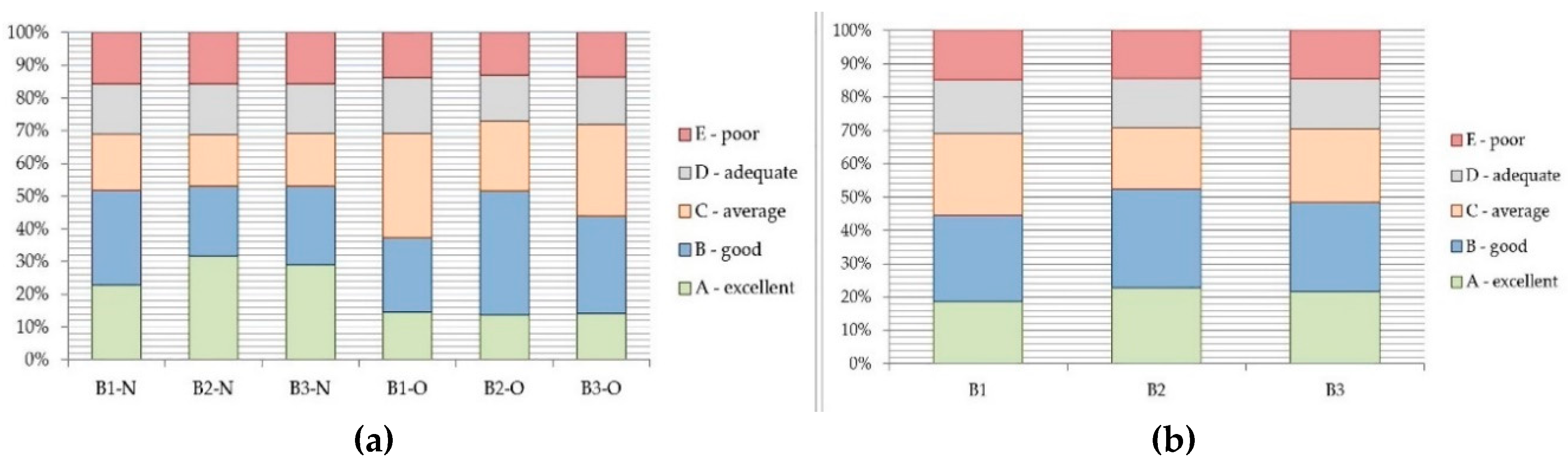
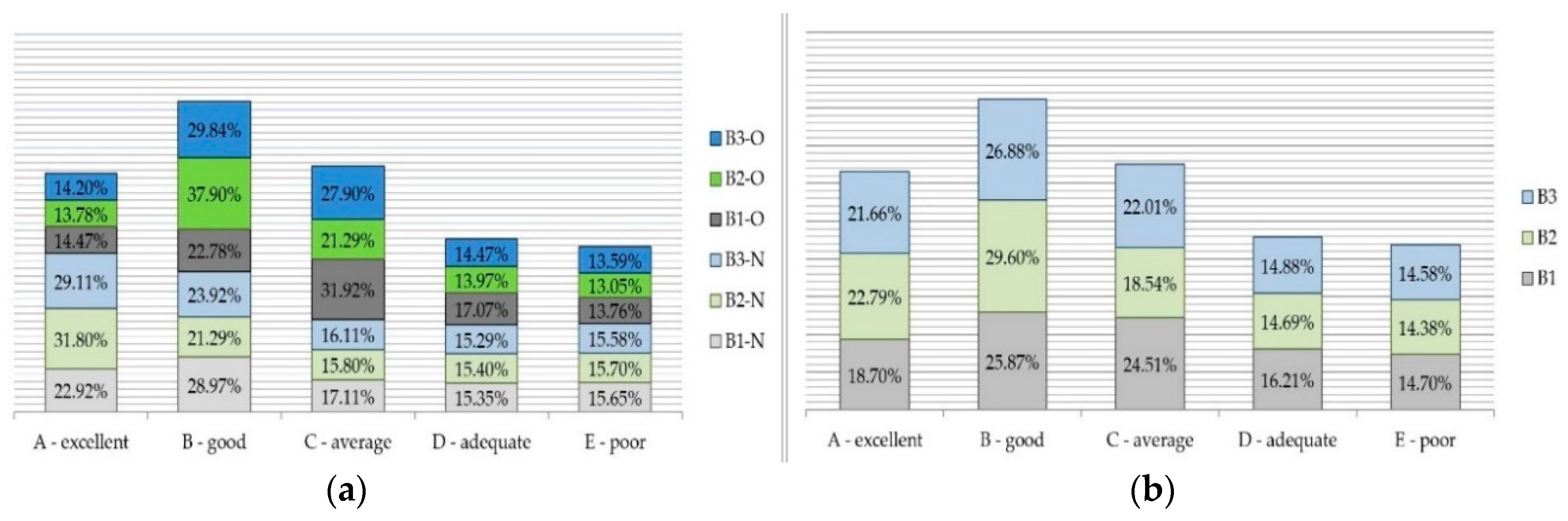
No corresponding combinations were recorded for other values of J_c.

(vii) In each of the above five groups of outcomes (vi), the highest, maximum value of the affiliation function among the corresponding minimums is sought (v):

$$\begin{array}{l}M{X}_{Jc=6}=\max {\left\{0.0125,\dots 0.158333\right\}}_{Jc=6}=0.25\\ M{X}_{Jc=7}=\max {\left\{0.0125,\dots 0.25\right\}}_{Jc=7}=0.475\\ M{X}_{Jc=8}=\max {\left\{0.0125,\dots 0.45\right\}}_{Jc=8}=0.525\\ M{X}_{Jc=9}=\max {\left\{0.0125,\dots 0.25\right\}}_{Jc=9}=0.525\\ M{X}_{Jc=10}=\max {\left\{0.25,\dots 0.25\right\}}_{Jc=10}=0.25\end{array}$$

The final expression for membership function of A of machine B1-N is derived in the form:

$$\mu A(B1-N)=(0,0,0,0,0,0.25,0.475,0.525,0.525,0.25)$$

(22)

Assessments for other machines are given below:

$$\begin{array}{l}\begin{array}{l}{\mu }_{A\left(B2-N\right)}=\left(0,0,0,0,0,0.2,0.3,0.525,0.525,0.4\right)\hfill \\ {\mu }_{A\left(B3-N\right)}=\left(0,0,0,0,0,0.1583,0.375,0.475,0.525,0.525\right)\hfill \\ {\mu }_{A\left(B1-O\right)}=\left(0,0,0.1,0.3625,0.1,0.2875,0.15,0.15,0.3,0\right)\hfill \\ {\mu }_{A\left(B2-O\right)}=\left(0,0,0,0.1,0.2,0.425,0.7167,0.65,0.15,0.125\right)\hfill \end{array}\\ {\mu }_{A\left(B3-O\right)}=\left(0,0,0,0.05,0.2667,0.675,0.675,0.55,0.3,0\right)\end{array}$$

3.4. Identification

To obtain the final ‘A’ grade for machine B1-N, the best-fit identification method was used as follows:

$$\begin{array}{l}{d}_{1(A(B1-N),\prime \mathrm{A}\prime )}=\sqrt{{\displaystyle \sum \begin{array}{c}j=10\\ j=1\end{array}{\left({\mu }_{A(B1-N)}^j-{\mu }_A^j\right)}^2}}\\ =\sqrt{{(0-0)}^2+\dots +{(0-0)}^2+{(0.25-0)}^2+{(0.475-0)}^2+{(0.525-0)}^2+{(0.25-1)}^2}=1.16270\end{array}$$

where μ_A(B1-N) according to (22) and μ_A according to (2)

For other fuzzy sets:

$$\begin{array}{l}{d}_{2(A(B1-N),\prime \mathrm{B}\prime )}=0.91996,d_{3(A(B1-N),\prime C\prime )}=1.55784,\\ d_{4(A(B1-N),\prime \mathrm{D}\prime )}=1.73580,d_{5(A(B1-N),\prime E\prime )}=1.70349.\end{array}$$

For d_min = d₂:

$${\mu }_1=\frac{d_{\min }}{d_1\cdot {\displaystyle {\sum }_{i=1}^{i=5}\frac{d_{\min }}{d_i}}}=\frac{0.91996}{\left(1.16270\cdot \left(\frac{0.91996}{1.16270}+\frac{0.91996}{0.91996}+\frac{0.91996}{1.55784}+\frac{0.91996}{1.73580}+\frac{0.91996}{1.70349}\right)\right)}=0.22922$$

Other values are: μ₂ = 0.28970, μ₃ = 0.17108, μ₄ = 0.15354, μ₅ = 0.15645

Finally, the grade of availability (15) of machine B1-N is recorded in the form:

A_(B1-N) = (0.22922/’A’, 0.28970/’B’, 0.17108/’C’, 0.15354/’D’, 0.15645/’E’)

If we designate grade ‘A’ as excellent availability, ‘B’ as good availability, ‘C’ as average availability, ‘D’ as adequate, ‘E’ as poor availability, Equation (15) can be interpreted as follows:

Machine B1-N was mostly assessed with good availability at a level of 29%, with a tendency towards excellent availability where the rating level is 23%. Lower grades are represented with 17% for good, 15% for satisfactory and poor availability. If the input grades are analyzed (Table 7), it can be seen that supportability (S) is most likely a contributory factor to the high availability rating for this machine. Following the above-presented method, availability estimates for other bulldozers are obtained (

Table 8. Assessment of bulldozer availability by expert’s judgment.

Machine	‘A’—Excellent	‘B’—Good	‘C’—Average	‘D’—Adequate	‘E’—Poor
B1-N	0.22922	0.28970	0.17108	0.15354	0.15645
B2-N	0.31801	0.21294	0.15800	0.15400	0.15705
B3-N	0.29108	0.23916	0.16110	0.15290	0.15576
B1-O	0.14472	0.22777	0.31916	0.17073	0.13762
B2-O	0.13784	0.37904	0.21289	0.13971	0.13052
B3-O	0.14204	0.29836	0.27904	0.14466	0.13591

).

3.5. Results Discussion

Figure 4 shows a comparative analysis of the availability of all six machines. It can be seen that the evaluation of new machines is predominantly excellent and good (‘A’ + ‘B’ > 50%). For the old machines, this is only the case for machine B2-O. For the new machines, B2-N is best rated, and for the old B2-O. For all machines, the least represented grades are adequate and poor availability (‘D’ + ‘E’ < 32%). The second chart on the same figure represents analysis in relation to bulldozer models. It is shown that the average availability grades are the highest (‘A’ + ‘B’) for the B2 machine. Figure 5 shows a comparative analysis of the grades, it can be seen that the dominant grade is ‘B’.

At the beginning of point 3, an availability analysis was obtained based on the time state picture. According to this analysis, availability is the highest for bulldozer B2, which is in accordance with the expert analysis presented here.

For the purpose of a more precise comparative analysis of the obtained results, the assessments (18) can be defuzzificated by the center of mass point calculation Z (Bowles and Pelaez, 1995). For machine B1-N, the calculation would have the following form:

$$Z_{B1-N}=\frac{{\displaystyle {\sum }_{i=1}^{i=5}}{\mu }_i\cdot I}{{\displaystyle {\sum }_{i=1}^{i=5}{\mu }_i}}=\frac{0.22922\cdot 5+0.28970\cdot 4+0.17108\cdot 3+0.15354\cdot 2+0.15645\cdot 1}{0.22922+0.28970+0.17108+0.15354+0.15645}=3.28$$

For the other machines, the parameter Z will be:

Z_B2-N = 3.38, Z_B3-N = 3.36, Z_B1-O = 3.07, Z_B2-O = 3.25, Z_B3-O = 3.17,

Respectively:

Z_B1 = 3.18, Z_B2 = 3.32, Z_B3 = 3.26

where I is the numerical equivalent of linguistic variables, 5-‘A’, … 1-‘E’.

The case study of EPS lignite mines has shown that according to specific working conditions the best choice of bulldozer is Caterpillar D8R (B2). On the scale from 1 to 5 (i.e., from poor to excellent availability), B2 is the best rated, and the worst rated machine is B1. The defined analysis concludes that this machine is the optimal selection, which may be a suggestion for the management of the company in future procurement.

4. Conclusions

In this paper, the expert assessment of the availability model is presented. In the conventional model (1–4), time periods (Figure 1) are used as input data rather than availability indicators. The expert model showed results that have the same tendency as measured availability values (Table 3), where Caterpillar bulldozer is better than the other two types. Availability is presented as a comprehensive indicator of the usability of a technical system affected by reliability, maintenance, and level of support. The descriptive form contains linguistic descriptions and affiliation (grade extent in a range of 0%–100%). Unlike the conventional model, the final grade can be divided into several outcomes. The synthesis was made using the fuzzy theory and the AHP ranking model. The model is illustrated using the example of the bulldozer. Verification was made by comparing the results of the new model and the conventional method of calculating availability.

The fuzzy-AHP model has an advantage over conventional models because it shows the importance of partial availability indicators. The final grade is in the descriptive form and depicts a tendency, so it is not given in the form of the number only. The necessary data for this model are the expert assessments of employees in the operation and maintenance of the machine, unlike the conventional model, which requires an IT monitoring system, in practice often unavailable, for the input data.

The paper presents the model by analyzing both old and new versions of three types of bulldozers operating in an open-pit mine for the exploitation of lignite. The analysis in this way provides guidance for selection and purchase, searching for weaknesses as well as the management of spare parts. Such an analysis is very important for large industrial complexes such as mines.

A possible recommendation for the company management is that the activities on maintenance analysis, operation analysis, weak-points analysis, and life cycle analysis adapt to this model, which effectively provides comparative data analysis. The model is easy to use. It can also be used for other systems, with possible corrections in the description of linguistic values.

References

1. Papic, L.; Milovanovic, Z.N. Systems Maintainability and Reliability; The Research Center of Dependability and Quality Management DQM: Prijevor, Serbia, 2007. [Google Scholar]
2. Dhillon, B.S. Mining Equipment Reliability, Maintainability and Safety; Springer: London, UK, 2008. [Google Scholar]
3. Todorovic, J. Maintainability Engineering; JUMV: Belgrade, Serbia, 1993. [Google Scholar]
4. Conlon, J.C.; Lilius, W.A.; Tubbesing, F.H., Jr. Test and Evaluation of System Reliability, Availability and Maintainability, A Primer; No. DOD-3235.1-H; Department of Defense: Washington, DC, USA, 1982. [Google Scholar]
5. International Electrotechnical Commission. INTERNATIONAL STANDARD IEC—Dependability Management 60300, 2003–01. Available online: https://webstore.iec.ch/preview/info_iec60300-3-1%7Bed2.0%7Den.pdf (accessed on 16 October 2019).
6. Strandberg, K. IEC 300: The Dependability Counterpart of ISO 9000. In Proceedings of the Annual Reliability and Maintainability Symposium, Orlando, FL, USA, 29–31 January 1991; pp. 463–467. [Google Scholar]
7. Avizienis, A.; Laprie, J.C.; Randell, B.; Landwehr, C. Basic concept and taxonomy of dependable and secure computing. IEEE Trans. Dependable Secur. Comput. 2004, 1, 11–33. [Google Scholar] [CrossRef]
8. Avizienis, A.; Laprie, J.; Randell, B. Dependability and its threats—A taxonomy. In IFIP Congress Topical Sessions; Springer: Boston, MA, USA, 2004; pp. 91–120. [Google Scholar]
9. Cai, K.Y. System failure engineering and fuzzy methodology an introductory overview. Fuzzy Sets Syst. 1996, 83, 113–133. [Google Scholar] [CrossRef]
10. Miodragovic, R.; Tanasijevic, M.; Mileusnic, Z.; Jovancic, P. Effectiveness assessment of agricultural machinery based on fuzzy sets theory. Expert Syst. Appl. 2012, 39, 8940–8946. [Google Scholar] [CrossRef]
11. Ebramhimipour, V.; Suzuki, K. A synergetic approach for assessing and improving equipment performance in offshore industry based on dependability. Reliab. Eng. Syst. Saf. 2006, 91, 10–19. [Google Scholar] [CrossRef]
12. Ivezic, D.; Tanasijevic, M.; Ignjatovic, D. Fuzzy Approach to Dependability Performance Evaluation. Qual. Reliab. Eng. Int. 2008, 24, 779–792. [Google Scholar] [CrossRef]
13. Tanasijevic, M.; Ivezic, D.; Jovancic, P.; Catic, D.; Zlatanovic, D. Study of Dependability Evaluation for Multi-hierarchical Systems Based on Max–Min Composition. Qual. Reliab. Eng. Int. 2013, 29, 317–326. [Google Scholar] [CrossRef]
14. Tanasijevic, M.; Ivezic, D.; Jovancic, P.; Ignjatovic, D.; Bugaric, U. Dependability assessment of open-pit mines equipment—Study on the bases of fuzzy algebra rules. Eksploat. Niezawodn. Maint. Reliab. 2013, 15, 66–74. [Google Scholar]
15. Jones, J.V. Supportability Engineering Handbook; Introduction Chapter; McGraw-Hill Education: New York, NY, USA, 2007. [Google Scholar]
16. Erkoyuncu, J.A.; Khan, S.; Eiroa, A.L.; Butler, N.; Rushton, K.; Brocklebank, S. Perspectives on trading cost and availability for corrective maintenance at the equipment type level. Reliab. Eng. Syst. Saf. 2017, 168, 53–69. [Google Scholar] [CrossRef]
17. Klir, G.J.; Yuan, B. Fuzzy Sets and Fuzzy Logic, Theory and Applications; Prentice Hall: New York, NY, USA, 1995; ISBN 0-13-101171-5. [Google Scholar]
18. Djuric, R.; Milisavljevic, V. Investigation on the relationship between reliability of track mechanism and dust content in rocks of lignite open pits. Maint. Reliab. 2016, 18, 142–150. [Google Scholar] [CrossRef]
19. Tanasijevic, M. A fuzzy-based decision support model for evaluation of mining machinery. In Proceedings of the 48th International October Conference on Mining and Metallurgy, Bor, Serbia, 28 September–1 October 2016; pp. 15–18. [Google Scholar]
20. Ivezic, D.; Tanasijevic, M.; Jovancic, P.; Djuric, R. A Fuzzy Expert Model for Availability Evaluation. In Proceedings of the 20th International Carpathian Control Conference (ICCC), Kraków-Wieliczka, Poland, 26–29 May 2019; ISBN 978-1-7281-0701-1. [Google Scholar]
21. Saaty, T.L. Decision Making: The Analytical Hierarchy Process; Mc-Graw-Hill: New York, NY, USA, 1980. [Google Scholar]
22. Jankovic, I.; Djenadic, S.; Ignjatovic, D.; Jovancic, P.; Subaranovic, T.; Ristovic, I. Multi-Criteria Approach for Selecting Optimal Dozer Type in Open-Cast Coal Mining. Energies 2019, 12, 2245. [Google Scholar] [CrossRef]
23. Karimnia, H.; Bagloo, H. Optimum mining method selection using fuzzy analytical hierarchy process-Qapiliq salt mine, Iran. Int. J. Min. Sci. Technol. 2015, 25, 225–230. [Google Scholar] [CrossRef]
24. Saaty, T.L. Decision making with the analytical hierarchy process. Int. J. Serv. Sci. 2008, 1, 83–98. [Google Scholar] [CrossRef]
25. Djenadic, S.; Miletic, F.; Jovancic, P.; Jankovic, I.; Lazic, M. Analitičko hijerarhijski proces primenjen za selekciju hidrauličnih bagera na površinskim kopovima. In Proceedings of the VIII Međunarodna Konferencija OMC 2018, Zlatibor, Serbia, 17–20 October 2018; Jugoslovenski komitet za površinsku eksploataciju: Belgrade, Serbia; pp. 14–16. [Google Scholar]
26. Stevanovic, D.; Lekic, M.; Krzanovic, D.; Ristovic, I. Application of MCDA in selection of different mining methods and solutions. Res. J. 2018, 12, 171–180. [Google Scholar] [CrossRef]
27. Milentijevic, G.; Nedeljkovic, B.; Lekic, M.; Nikic, Z.; Ristović, I.; Djokic, J. Application of a Method for Intelligent Multi-Criteria Analysis of the Environmental Impact of Tailing Ponds in Northern Kosovo and Metohija. Energies 2016, 9, 935. [Google Scholar] [CrossRef]
28. Saaty, T.L. Fundamentals of Decision Making and Priority Theory with the Analytic Hierarchy Process; RWS Publications: Pittsburgh, PA, USA, 2000. [Google Scholar]
29. Djenadic, S.; Jovancic, P.; Ignjatovic, D.; Miletic, F.; Jankovic, I. Analiza primene višekriterijumskih metoda u optimizaciji izbora hidrauličnih bagera na površinskim kopovima. Tehnika 2019, 70, 369–377. [Google Scholar] [CrossRef]
30. Ignjatovic, D.; Jovancic, P. Optimisation of Operation and Costs of Auxiliary Mechanization in Order to Increase the Utilization of Overburden and Coal Systems on the Open-Cast Mines of Electrical Power Supply of Serbia—Research Study; Faculty of Mining and Geology: Belgrade, Serbia, 2018. [Google Scholar]
Figure 1. Time state picture. t1, uptime; t11, standby time; t12, time in operation; t2, downtime; t21, organizational time; t22, logistic time; t23, repair time (t231, corrective; t232, preventive repair).
Energies 12 04044 g001
Figure 2. The ratio of reliability R(t) and availability A(t).
Energies 12 04044 g002
Figure 3. Dependence of linguistic variables and membership function, the general form.
Energies 12 04044 g003
Figure 4. Comparative analysis of all bulldozers availability and analysis according to different models. (a) for all of the analysed machines; (b) for machines according to manufacturer.
Energies 12 04044 g004
Figure 5. Comparative analysis of bulldozer availability according to different grades. (a) for all of the analysed machines; (b) for machines according to manufacturer.
Energies 12 04044 g005