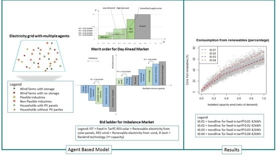
Assessing Financial and Flexibility Incentives for Integrating Wind Energy in the Grid Via Agent-Based Modeling
Abstract
1. Introduction
1.1. Electricity Markets and Grid Balancing
1.2. Hypothesis Formulation
2. Methodology
2.1. Developing the ABM
2.1.1. Purpose
2.1.2. Entities, State Variables and Scales
- a.
- RES-E producers (2 groups)
- Non-storing producers: RE producers who do not own storage but in cases of grid imbalance can curtail their production.
- Storing producers: Storing RES-E producers who can store electricity when the actual supply exceeds nominated supply. They provide the stored electricity and the available storage capacity as reserves on the IM.
- b.
- Large industries (4 groups)
- Group 0—non-flex: Industries that do not engage in the IM.
- Group 1—cheap reserves: industries that provide reserves at a symmetric price of 0.04 €/kWh.
- Group 2—mid-priced reserves: industries that provide reserves at a symmetric price of 0.08 €/kWh.
- Group 3—expensive reserves: industries that provide reserves at a symmetric price of 0.14 €/kWh.
- c.
- Small or medium sized consumers (SMCs) (2 groups)
- Prosumers: SMCs with PV panels,
- Consumers: SMCs without PV panels.
- d.
- Electricity markets
2.1.3. Process Overview and Scheduling
- Predicting consumption and production for the next day,
- Setting a DAM price for each hour of the day,
- Actual consumption and production in every quarter,
- Calculating the system imbalance to decide to engage the IM,
- Based on the imbalance, setting the IM price for every 15 min,
- Updating the system variables,
- Calculating profit,
- Storing the unitary profit producers at the end of every month,
- Storing the unitary bill of SMCs and industries at the end of every month,
- Changing behavior based on the comparison of unitary bill and unitary profit with other agents in the past three months,
- At the end of the year, calculate the bill for SMCs.
2.2. Statistical Analysis
3. Results
3.1. Effect on the RES-E Consumption
3.2. Effect on the Market Prices
3.3. Effect on Different Agents
4. Discussion
5. Conclusions
Author Contributions
Funding
Acknowledgments
Conflicts of Interest
Appendix A. Methodology
| Definition | Values | Unit | |
|---|---|---|---|
| Small and medium sized consumers | |||
| Agent properties (do not change during the simulation runs) | |||
| consumption capacity of a household [41] | 0.125 | kWh | |
| capacity of a photovoltaic panel [41] | 1–2 | kWh | |
| Agent Variables (may change in every time step) | |||
| predicted consumption for one quarter of an hour on the next day | |||
| actual consumption in real time | |||
| random.factor | a number generated every quarter of an hour to introduce randomness in the consumption profile of the consumers | 0.01–0.05 | |
| production from the photovoltaic panels in real time | |||
| consumption from own PV panel (only for prosumers) | |||
| production from the PV-panels in real time that is planned for the | |||
| bill for the whole past year | € | ||
| per unit cost of electricity consumed in the past year | €/kWh | ||
| Industry | |||
| Agent properties (do not change during the simulation runs) | |||
| average consumption of an industry | 2000 (±400) | kWh | |
| group | group number defining the strategy of the industry Group 0: bid-cap of 0 kW Group 1, 2, and 3: bid-cap of 50% of | 0–3 | |
| Agent variables (may change in every time step) | |||
| predicted consumption for one quarter of an hour on the next day | |||
| actual consumption in real time | |||
| for group 0, for group 1, for group 2, for group 3, | |||
| for group 0, for group 1,2, and 3, | |||
| total consumption in the past month | kWh | ||
| bidding capacity (flexible demand) | 50% of | kW | |
| bill for the past month | € | ||
| instantaneous profit in every time step | € | ||
| unitary profit for the past month | €/kWh | ||
| RES-E Producers | |||
| Agent properties (do not change during the simulation runs) | |||
| average production capacity of a wind farm | 4000 (±100) | kW | |
| average storage capacity | 20% of | kW | |
| costs for curtailing [61] | 0.022 | €/kWh | |
| LCOE 1 of battery storage [62] | 0.176 | €/kWh | |
| strategy | strategy defining if the producer will have storage or not If 0, there is no storage facility If 1, there is storage facility | 0 or 1 | |
| Agent variables (may change in every time step) | |||
| Required production per agent to meet the system demand | kWh | ||
| nominated power production for the next day | kWh | ||
| actual power production in real time | kWh | ||
| part or all of the made available for the system | kWh | ||
| curtailed power | kWh | ||
| stored power in real time | kWh | ||
| production sold at the DAM 2, | kWh | ||
| production bid at the IM 3 | kWh | ||
| production sold at the IM If, | kWh | ||
| kWh | |||
| total production traded in the markets in the past month | kWh | ||
| storage reserve engaged by IM. Value is positive when batteries are discharged, and negative when batteries are charged | kWh | ||
| instantaneous profit in every time step | € | ||
| unitary profit for the past month | €/kWh | ||
Appendix A.1. Sub-Models
Appendix A.1.1. Prediction of Consumption and Production
Appendix A.1.2. Setting the Day Ahead Market Price
Appendix A.1.3. Actual Consumption and Production
Appendix A.1.4. Setting the Imbalance Market Price

Appendix A.1.5. Calculating Profit for Industries and RES-E Producers
Appendix A.1.6. Updating the System Variables
Appendix A.1.7. Changing Strategies
Appendix A.1.8. Calculating Bill for the SMCs
Appendix A.2. Design Concepts
- Number of industries,
- Number of RES-E producers,
- Averaged unitary profit of RES-E producers,
- Averaged unitary profit of industries,
- Averaged unitary bill of consumers,
- Averaged unitary bill of prosumers,
- Annual DAM price,
- Annual IM price,
- Percentage of system consumption from renewables.
Appendix A.3. Initialization
Appendix A.4. Input Data
- V = Wind speed, m/s,
- Cp = 0.59 (theoretical maximum),
- ρ = Air density, kg/m3,
- A = Rotor swept area, m2 or π D2/4.
- A = area of a solar panel (assumed to be 10 m2 on average),
- r = solar panel yield (assumed to be 40%),
- Performance Ratio (PR) = 0.75 (default value),
- H = average quarter hourly solar radiation (kW/m2).
Appendix B. Results
| Equation (1) | 95% Confidence Intervals | Standard Error | p-Values |
| Intercept | [7.6100895, 8.7469286] | 0.28994 | <2 × 10⁻¹⁶ |
| [53.9763258, 55.9404355] | 0.50093 | <2 × 10⁻¹⁶ | |
| [−0.9897179, 0.6180155] | 0.41004 | 0.65039 | |
| [−0.6306872, 0.9770462] | 0.41004 | 0.67279 | |
| [0.2593658, 1.8670992] | 0.41004 | 0.00954 | |
| [1.5699873, 3.1777207] | 0.41004 | 7.5 × 10⁻⁹ | |
| [−1.3081767, 1.4694938] | 0.70843 | 0.90936 | |
| [−2.1174333, 0.6602372] | 0.70843 | 0.30378 | |
| [−1.8649325, 0.9127379] | 0.70843 | 0.50159 | |
| [9.9443263, 12.7219968] | 0.70843 | <2 × 10⁻¹⁶ | |
| Equation (2) | 95% Confidence Intervals | Standard Error | p-Values |
| Intercept | [2.7071620, 3.9960798] | 0.3286 | <2 × 10⁻¹⁶ |
| [74.5869387, 81.0400927] | 1.6451 | <2 × 10⁻¹⁶ | |
| [−1.2862439, 0.5365611] | 0.4647 | 0.420 | |
| [−1.1963856, 0.6264195] | 0.4647 | 0.540 | |
| [−0.348558, 1.4742464] | 0.4647 | 0.226 | |
| [−0.4867967, 1.3360083] | 0.4647 | 0.361 | |
| [−2.7162018, 6.4099361] | 2.3265 | 0.427 | |
| [−2.2348564, 6.8912815] | 2.3265 | 0.317 | |
| [−1.8526038, 7.2735342] | 2.3265 | 0.244 | |
| [15.6178810, 24.7440189] | 2.3265 | <2 × 10⁻¹⁶ | |
| Equation (3) | 95% Confidence Intervals | Standard Error | p-Values |
| Intercept | [14.484822, 16.918209] | 0.6205 | <2 × 10⁻¹⁶ |
| [42.828969, 46.291382] | 0.8830 | <2 × 10⁻¹⁶ | |
| [−2.367283, 1.074046] | 0.8776 | 0.461 | |
| [−1.602670, 1.838659] | 0.8776 | 0.893 | |
| [−0.585964, 2.855365] | 0.8776 | 0.196 | |
| [4.022200, 7.463529] | 0.8776 | 6.94 × 10⁻¹⁶ | |
| [−1.777742, 3.118849] | 1.2487 | 0.591 | |
| [−3.148456, 1.748135] | 1.2487 | 0.575 | |
| [−3.067230, 1.829361] | 1.2487 | 0.620 | |
| [4.248845, 9.145436] | 1.2487 | 8.74 × 10⁻⁸ | |
| Equation (4) | 95% Confidence Intervals | Standard Error | p-Values |
| Intercept | [0.0249092567, 0.0250611015] | 3.873 × 10⁻⁵ | <2 × 10⁻¹⁶ |
| [0.0131371212, 0.0133994625] | 6.691 × 10⁻⁵ | <2 × 10⁻¹⁶ | |
| [−0.0007381475, −0.0005234065] | 5.477 × 10⁻⁵ | <2 × 10⁻¹⁶ | |
| [−0.0013410582, −0.0011263171] | 5.477 × 10⁻⁵ | <2 × 10⁻¹⁶ | |
| [−0.0020040095, −0.0017892684] | 5.477 × 10⁻⁵ | <2 × 10⁻¹⁶ | |
| [−0.0023555315, −0.0021407904] | 5.47 × 10⁻⁵ | <2 × 10⁻¹⁶ | |
| [−0.0035230511, −0.0031520444] | 9.462 × 10⁻⁵ | <2 × 10⁻¹⁶ | |
| [−0.0068965095, −0.0065255028] | 9.462 × 10⁻⁵ | <2 × 10⁻¹⁶ | |
| [−0.0102137379, −0.0098427312] | 9.462 × 10⁻⁵ | <2 × 10⁻¹⁶ | |
| [−0.0141593139, −0.0137883072] | 9.462 × 10⁻⁵ | <2 × 10⁻¹⁶ | |
| Equation (5) | 95% Confidence Intervals | Standard Error | p-Values |
| Intercept | [0.0249092567, 0.0250611015] | 0.0002107 | <2 × 10⁻¹⁶ |
| [0.0131371212, 0.0133994625] | 0.0003641 | <2 × 10⁻¹⁶ | |
| [−0.0007381475, −0.0005234065] | 0.0002980 | 0.160095 | |
| [−0.0013410582, −0.0011263171] | 0.0002980 | 0.002045 | |
| [−0.0020040095, −0.0017892684] | 0.0002980 | 0.000215 | |
| [−0.0023555315, −0.0021407904] | 0.0002980 | <2 × 10⁻¹⁶ | |
| [−0.0035230511, −0.0031520444] | 0.0005149 | 0.049849 | |
| [−0.0068965095, −0.0065255028] | 0.0005149 | 3.79 × 10⁻⁵ | |
| [−0.0102137379, −0.0098427312] | 0.0005149 | 1.88 × 10⁻¹¹ | |
| [−0.0141593139, −0.0137883072] | 0.0005149 | <2 × 10⁻¹⁶ | |
| Equation (6) | 95% Confidence Intervals | Standard Error | p-Values |
| Intercept | [0.0009089505, 1.518687 × 10⁻³] | 1.554 × 10⁻⁴ | 1.20 × 10⁻¹⁴ |
| [0.0009249548, 5.236665 × 10⁻³] | 1.099 × 10⁻³ | 0.00513 | |
| [−0.0005317846, 3.305135 × 10⁻⁴] | 2.198 × 10⁻⁴ | 0.64709 | |
| [−0.0004843669, 3.779311 × 10⁻⁴] | 2.198 × 10⁻⁴ | 0.80870 | |
| [−0.0007923893, 6.990876 × 10⁻⁵] | 2.198 × 10⁻⁴ | 0.10048 | |
| [0.0023973214, 3.259619 × 10⁻³] | 2.198 × 10⁻⁴ | <2 × 10⁻¹⁶ | |
| [−0.0056389054, 4.587736 × 10⁻⁴] | 1.554 × 10⁻³ | 0.09583 | |
| [−0.0094620968, −3.364418 × 10⁻³] | 1.554 × 10⁻³ | 3.92 × 10⁻¹⁶ | |
| [−0.0105595729, −4.461894 × 10−43] | 1.554 × 10⁻³ | 1.51 × 10⁻⁶ | |
| [0.0083587361, 1.445642 × 10⁻²] | 1.554 × 10⁻³ | 3.84 × 10⁻¹³ | |
| Equation (7) | 95% Confidence Intervals | Standard Error | p-Values |
| Intercept | [0.009186941, 0.0106329549] | 0.0003688 | <2 × 10⁻¹⁶ |
| [−0.035489722, −0.0333098310] | 0.0005559 | <2 × 10⁻¹⁶ | |
| [−0.001799072, 0.0002459000] | 0.0005215 | 0.136548 | |
| [−0.002920207, −0.0008752344] | 0.0005215 | 0.000278 | |
| [−0.002860245, −0.0008152728] | 0.0005215 | 0.000430 | |
| [0.003440509, 0.0054854812] | 0.0005215 | <2 × 10⁻¹⁶ | |
| [−0.002047464, 0.0010353664] | 0.0007862 | 0.519831 | |
| [−0.002286895, 0.0007959363] | 0.0007862 | 0.343084 | |
| [−0.003969384, −0.0008865529] | 0.0007862 | 0.002028 | |
| [0.006221606, 0.0093044372] | 0.0007862 | <2 × 10⁻¹⁶ |
References
- European Commission. Renewable Energy Statistics—Eurostat Statistics Explained. Available online: https://ec.europa.eu/eurostat/statistics-explained/index.php/Renewable_energy_statistics (accessed on 3 June 2019).
- European Commission. Directive (EU) 2018/2001 of the European Parliament and of the Council of 11 December 2018 on the Promotion of the Use of Energy from Renewable Sources; European Commission: Brussels, Belgium, 2018. [Google Scholar]
- WindEurope.org. Wind Energy in Europe in 2018. Available online: https://windeurope.org/wp-content/uploads/files/about-wind/statistics/WindEurope-Annual-Statistics-2018.pdf (accessed on 16 May 2019).
- Fanone, E.; Gamba, A.; Prokopczuk, M. The case of negative day-ahead electricity prices. Energy Econ. 2013, 35, 22–34. [Google Scholar] [CrossRef]
- Brandstätt, C.; Brunekreeft, G.; Jahnke, K. How to deal with negative power price spikes?—Flexible voluntary curtailment agreements for large-scale integration of wind. Energy Policy 2011, 39, 3732–3740. [Google Scholar] [CrossRef]
- De Vos, K. Negative Wholesale Electricity Prices in the German, French and Belgian Day-Ahead, Intra-Day and Real-Time Markets. Electr. J. 2015, 28, 36–50. [Google Scholar] [CrossRef]
- Lund, P.D. Effects of energy policies on industry expansion in renewable energy. Renew. Energy 2009, 34, 53–64. [Google Scholar] [CrossRef]
- Peak Gen Power. Available online: https://www.peakgen.com/ (accessed on 5 August 2019).
- WindEurope.org. Making Transition Work; WindEurope: Brussels, Belgium, 2016. [Google Scholar]
- Kim, J.-H.; Shcherbakova, A. Common failures of demand response. Energy 2011, 36, 873–880. [Google Scholar] [CrossRef]
- Paulus, M.; Borggrefe, F. The potential of demand-side management in energy-intensive industries for electricity markets in Germany. Appl. Energy 2011, 88, 432–441. [Google Scholar] [CrossRef]
- Qadrdan, M.; Cheng, M.; Wu, J.; Jenkins, N. Benefits of demand-side response in combined gas and electricity networks. Appl. Energy 2017, 192, 360–369. [Google Scholar] [CrossRef]
- National Grid ESO. Power Responsive Steering Group by National Grid Electricity System Operator; and the Environmental Charity Sustainability First. In Power Responsive: Demand Side Flexibility; Annual Report; National Grid ESO: Gallows Hill, UK, 2018. [Google Scholar]
- Li, G.; Shi, J. Agent-based modeling for trading wind power with uncertainty in the day-ahead wholesale electricity markets of single-sided auctions. Appl. Energy 2012, 99, 13–22. [Google Scholar] [CrossRef]
- Sopha, B.M.; Klöckner, C.A.; Hertwich, E.G. Adoption and diffusion of heating systems in Norway: Coupling agent-based modeling with empirical research. Environ. Innov. Soc. Transit. 2013, 8, 42–61. [Google Scholar] [CrossRef]
- Schramm, M.E.; Trainor, K.J.; Shanker, M.; Hu, M.Y. An agent-based diffusion model with consumer and brand agents. Decis. Support Syst. 2010, 50, 234–242. [Google Scholar] [CrossRef]
- Van Dam, K.H.; Nikolic, I.; Lukszo, Z. (Eds.) Agent-Based Modelling of Socio-Technical Systems; Springer Science & Business Media: Berlin/Heidelberg, Germany, 2012; Volume 9. [Google Scholar]
- Bellekom, S.; Arentsen, M.; van Gorkum, K. Prosumption and the distribution and supply of electricity. Energy Sustain. Soc. 2016, 6, 22. [Google Scholar] [CrossRef]
- Fichera, A.; Pluchino, A.; Volpe, R. A multi-layer agent-based model for the analysis of energy distribution networks in urban areas. Phys. A Stat. Mech. Appl. 2018, 508, 710–725. [Google Scholar] [CrossRef]
- Misra, S.; Bera, S.; Ojha, T.; Zhou, L. Entice: Agent-based energy trading with incomplete information in the smart grid. J. Netw. Comput. Appl. 2015, 55, 202–212. [Google Scholar] [CrossRef]
- North, M.; Conzelmann, G.; Koritarov, V.; Macal, C.; Thimmapuram, P.; Veselka, T. E-Laboratories: Agent-Based Modeling of Electricity Markets; Argonne National Lab.: Lemont, IL, USA, 2002. [Google Scholar]
- Vasirani, M.; Kota, R.; Cavalcante, R.L.G.; Ossowski, S.; Jennings, N.R. An Agent-Based Approach to Virtual Power Plants of Wind Power Generators and Electric Vehicles. IEEE Trans. Smart Grid 2013, 4, 1314–1322. [Google Scholar] [CrossRef]
- Lund, P.D.; Lindgren, J.; Mikkola, J.; Salpakari, J. Review of energy system flexibility measures to enable high levels of variable renewable electricity. Renew. Sustain. Energy Rev. 2015, 45, 785–807. [Google Scholar] [CrossRef]
- Elia. The Day-Ahead Hub: A Platform at the Centre of ARPs Activities; Elia: Brussels, Belgium, 2012. [Google Scholar]
- Balancing Mechanism—Elia. Available online: https://www.elia.be/en/products-and-services/balance/balancing-mechanism (accessed on 6 August 2019).
- Meyer, N.I. European schemes for promoting renewables in liberalised markets. Energy Policy 2003, 31, 665–676. [Google Scholar] [CrossRef]
- Menanteau, P.; Finon, D.; Lamy, M.-L. Prices versus quantities: Choosing policies for promoting the development of renewable energy. Energy Policy 2003, 31, 799–812. [Google Scholar] [CrossRef]
- Verhaegen, K.; Meeus, L.; Belmans, R. Towards an international tradable green certificate system—The challenging example of Belgium. Renew. Sustain. Energy Rev. 2009, 13, 208–215. [Google Scholar] [CrossRef]
- World Nuclear News. Belgium Maintains Nuclear Phase-Out Policy. Available online: https://www.world-nuclear-news.org/Articles/Belgium-maintains-nuclear-phase-out-policy (accessed on 8 Novmber 2019).
- Flemish Green Power Certificates (GSC)|Agency Innovation and Entrepreneurship. Available online: https://www.vlaio.be/nl/subsidies-financiering/subsidiedatabank/vlaamse-groenestroomcertificaten-gsc (accessed on 10 December 2018).
- Generating Facilities. Available online: https://www.elia.be/en/grid-data/power-generation/generating-facilities (accessed on 8 November 2019).
- Shum, K.L. Renewable energy deployment policy: A transition management perspective. Renew. Sustain. Energy Rev. 2017, 73, 1380–1388. [Google Scholar] [CrossRef]
- Ashok, S.; Banerjee, R. Load-management applications for the industrial sector. Appl. Energy 2000, 66, 105–111. [Google Scholar] [CrossRef]
- Baker, P. Benefiting Customers while Compensating Suppliers: Getting Supplier Compensation Right; The Regulatory Assistance Project (RAP): Brussels, Belgium, 2016. [Google Scholar]
- Grimm, V.; Berger, U.; DeAngelis, D.L.; Polhill, J.G.; Giske, J.; Railsback, S.F. The ODD protocol: A review and first update. Ecol. Model. 2010, 221, 2760–2768. [Google Scholar] [CrossRef]
- Wilensky, U. Netlogo; Northwestern University Evanston: Evanston, IL, USA, 1999. [Google Scholar]
- Grimm, V.; Berger, U.; Bastiansen, F.; Eliassen, S.; Ginot, V.; Giske, J.; Goss-Custard, J.; Grand, T.; Heinz, S.K.; Huse, G.; et al. A standard protocol for describing individual-based and agent-based models. Ecol. Model. 2006, 198, 115–126. [Google Scholar] [CrossRef]
- Borggrefe, F.; Neuhoff, K. Balancing and Intraday Market Design: Options for Wind Integration; DIW Discussion Papers; German Institute for Economic Research: Berlin, Germany, 2011. [Google Scholar]
- IRENA. Renewable Power Generation Costs in 2017; International Renewable Energy Agency: Abu Dhabi, UAE, 2018; p. 160. [Google Scholar]
- Kost, C.; Shammugam, S.; Jülch, V.; Nguyen, H.-T.; Schlegl, T. Levelized Cost of Electricity—Renewable Energy Technologies; Fraunhofer Institute for Solar Energy Systems ISE: Freiburg im Breisgau, Germany, 2013. [Google Scholar]
- Mulder, G.; Six, D.; Claessens, B.; Broes, T.; Omar, N.; Mierlo, J.V. The dimensioning of PV-battery systems depending on the incentive and selling price conditions. Appl. Energy 2013, 111, 1126–1135. [Google Scholar] [CrossRef]
- IRENA. Renewable Energy Prospects: 2014; International Renewable Energy Agency: Abu Dhabi, UAE, 2014. [Google Scholar]
- Masson, G.; Neubourg, G. PV Prosumer Guidelines Belgium; Becquerel Institute: Brussels, Belgium, 2019; p. 8. [Google Scholar]
- Alberici, S. Subsidies and Costs of EU Energy (Annex 4–5); Ecofys: Berlin, Germany, 2014. [Google Scholar]
- Government of Flanders Screen Flanders—Climate and Weather. Available online: https://www.screenflanders.be/en/film-commission/production-guide/facts-and-figures/climate-and-weather (accessed on 9 October 2019).
- Team, F. The Potential Role of H2 Production in a Sustainable Future Power System. Available online: https://ec.europa.eu/jrc/en/publication/potential-role-h2-production-sustainable-future-power-system (accessed on 21 October 2019).
- About Elia—Elia. Available online: http://www.elia.be/en/about-elia (accessed on 16 May 2019).
- R Core Team. R: A Language and Environment for Statistical Computing; R Foundation for Statistical Computing: Vienna, Austria, 2013. [Google Scholar]
- Cludius, J.; Hermann, H.; Matthes, F.C.; Graichen, V. The merit order effect of wind and photovoltaic electricity generation in Germany 2008–2016: Estimation and distributional implications. Energy Econ. 2014, 44, 302–313. [Google Scholar] [CrossRef]
- De Vos, K.; Petoussis, A.G.; Driesen, J.; Belmans, R. Revision of reserve requirements following wind power integration in island power systems. Renew. Energy 2013, 50, 268–279. [Google Scholar] [CrossRef]
- Kondoh, J.; Ishii, I.; Yamaguchi, H.; Murata, A.; Otani, K.; Sakuta, K.; Higuchi, N.; Sekine, S.; Kamimoto, M. Electrical energy storage systems for energy networks. Energy Convers. Manag. 2000, 41, 1863–1874. [Google Scholar] [CrossRef]
- Zhao, H.; Wu, Q.; Hu, S.; Xu, H.; Rasmussen, C.N. Review of energy storage system for wind power integration support. Appl. Energy 2015, 137, 545–553. [Google Scholar] [CrossRef]
- McDowall, J. Integrating energy storage with wind power in weak electricity grids. J. Power Sources 2006, 162, 959–964. [Google Scholar] [CrossRef]
- Frondel, M.; Sommer, S.; Vance, C. The burden of Germany’s energy transition: An empirical analysis of distributional effects. Econ. Anal. Policy 2015, 45, 89–99. [Google Scholar] [CrossRef]
- Winkler, J.; Altmann, M. Market Designs for a Completely Renewable Power Sector. Z. Energ. 2012, 36, 77–92. [Google Scholar] [CrossRef]
- Zwaenepoel, B.; Vansteenbrugge, J.; Vandoorn, T.L.; Van Eetvelde, G.; Vandevelde, L. Ancillary services for the electrical grid by waste heat. Appl. Therm. Eng. 2014, 70, 1156–1161. [Google Scholar] [CrossRef]
- Verzijlbergh, R.A.; De Vries, L.J.; Dijkema, G.P.J.; Herder, P.M. Institutional challenges caused by the integration of renewable energy sources in the European electricity sector. Renew. Sustain. Energy Rev. 2017, 75, 660–667. [Google Scholar] [CrossRef]
- Kikuchi, Y.; Kanematsu, Y.; Ugo, M.; Hamada, Y.; Okubo, T. Industrial Symbiosis Centered on a Regional Cogeneration Power Plant Utilizing Available Local Resources: A Case Study of Tanegashima. J. Ind. Ecol. 2016, 20, 276–288. [Google Scholar] [CrossRef]
- Rogers, E.M. Diffusion of Innovations, 4th ed.; Simon and Schuster: New York, NY, USA, 2010; ISBN 978-1-4516-0247-0. [Google Scholar]
- Larsen, J.K. Available online: https://studylib.net/doc/7736725/rocky-mountain-power-decision-summary-report-on-purpa-time (accessed on 8 November 2019).
- Joos, M.; Staffell, I. Short-term integration costs of variable renewable energy: Wind curtailment and balancing in Britain and Germany. Renew. Sustain. Energy Rev. 2018, 86, 45–65. [Google Scholar] [CrossRef]
- Wilson, M. Available online: https://www.lazard.com/media/450774/lazards-levelized-cost-of-storage-version-40-vfinal.pdf (accessed on 8 November 2019).




| Definition | Values | Unit | |
|---|---|---|---|
| Parameters (Do Not Change during the Simulation Runs) | |||
| LCOE 1 of photovoltaic panels calculated over 20 years period [42]. | 0.088 | €/kWh | |
| LCOE of wind turbines calculated over a time period of 20 years [42] | 0.053 | €/kWh | |
| feed-in tariffs given to RES-E 2 producers based on data from Belgium | 0–0.04 | €/kWh | |
| total production capacity of wind farms as a ratio of average system consumption. x represents the ratio | 0–100 | % | |
| wind | average wind velocity in Belgium [45] | 4 | m/s |
| price of electricity bought and sold to the backup technology that can balance the grid imbalances and is engaged a day ahead of actual supply. The hypothetical value of 0.1 €/kWh is considered because this is higher than the LCOE of photovoltaic panels but still comparable to LCOE of biogas power plants [40] | 0.1 | €/kWh | |
| sum of capacity provided by the cheap reserves | kWh | ||
| sum of capacity provided by the mid-priced reserves | kWh | ||
| sum of capacity provided by the expensive reserves | kWh | ||
| symmetric bidding price of electrolyzer. Depending on the country the price may vary [46] | 0.2 | €/kWh | |
| bidding price of RES-E from wind farms | 0.06 | €/kWh | |
| bidding price for the electricity provided or consumed by battery storage of wind farm owners | 0.18 | €/kWh | |
| capacity of inflexible power production system | 20% of average demand | kW | |
| capacity of the back-up system | kW | ||
| LCOE of inflexible hydro power production system | 0.02 | €/kWh | |
| sum of capacity provided by the flexible natural gas plant that participates in DAM 3 | 10% of average demand | kW | |
| LCOE of the flexible natural gas fired power plant [40] | 0.04 | €/kWh | |
| State variables (may change in every time step) | |||
| predicted wind intensity at that quarter on the next day | 0–1 | range | |
| predicted solar irradiation at that quarter on the next day | 0–1 | range | |
| predicted and engaged supply to meet the demand on DAM | kWh | ||
| predicted demand from the system on DAM | kWh | ||
| total predicted production from the wind farms | kWh | ||
| total predicted production from prosumers | kWh | ||
| total production from the wind farms in real time | kWh | ||
| supply in real time before balancing | kWh | ||
| demand in real time before balancing | kWh | ||
| day ahead market price of electricity | −0.15–0.15 | €/kWh | |
| wind intensity in real-time | 0–1 | range | |
| solar irradiation in real-time | 0–1 | range | |
| total production from the prosumers in real time | kWh | ||
| production from wind farms that has been made available to balance the grid at | kWh | ||
| production from storing agents that has been made available to balance the grid at | |||
| ratio of the RES-wind-act that is needed for activation on IM | % | ||
| capacity activated from the backup technology for balancing DAM | kWh | ||
| annual DAM price. | |||
| annual IM 4 price. | |||
| imbalance market price | −0.2–0.2 | €/kWh | |
| percentage of the total yearly demand of the system met by RES-E | 0–100 | % | |
© 2019 by the authors. Licensee MDPI, Basel, Switzerland. This article is an open access article distributed under the terms and conditions of the Creative Commons Attribution (CC BY) license (http://creativecommons.org/licenses/by/4.0/).
Share and Cite
Maqbool, A.S.; Baetens, J.; Lotfi, S.; Vandevelde, L.; Van Eetvelde, G. Assessing Financial and Flexibility Incentives for Integrating Wind Energy in the Grid Via Agent-Based Modeling. Energies 2019, 12, 4314. https://doi.org/10.3390/en12224314
Maqbool AS, Baetens J, Lotfi S, Vandevelde L, Van Eetvelde G. Assessing Financial and Flexibility Incentives for Integrating Wind Energy in the Grid Via Agent-Based Modeling. Energies. 2019; 12(22):4314. https://doi.org/10.3390/en12224314
Chicago/Turabian StyleMaqbool, Amtul Samie, Jens Baetens, Sara Lotfi, Lieven Vandevelde, and Greet Van Eetvelde. 2019. "Assessing Financial and Flexibility Incentives for Integrating Wind Energy in the Grid Via Agent-Based Modeling" Energies 12, no. 22: 4314. https://doi.org/10.3390/en12224314
APA StyleMaqbool, A. S., Baetens, J., Lotfi, S., Vandevelde, L., & Van Eetvelde, G. (2019). Assessing Financial and Flexibility Incentives for Integrating Wind Energy in the Grid Via Agent-Based Modeling. Energies, 12(22), 4314. https://doi.org/10.3390/en12224314


