1. Introduction
Over the last few years, the fourth industrial revolution has attracted more and more attention worldwide. Industry 4.0, or smart manufacturing, combines the strengths of traditional industries with new cutting edge technologies [
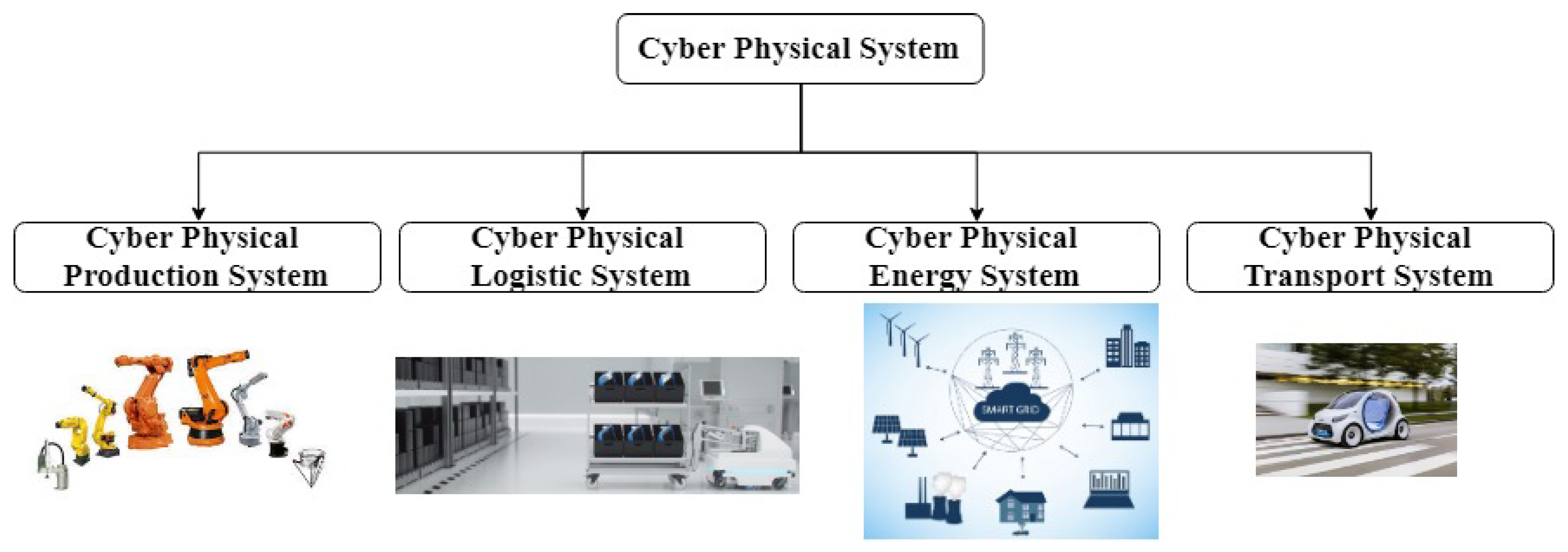
1]. It is the combination of several technological developments that embrace both products and processes. Manufacturing systems are converted into intelligent connected factories using new technologies such as cloud manufacturing, internet of things (IoT), cyber physical systems (CPS), big data analytics (BDA), and information and communication technologies (ICT). Networking, digitalization, and computing are keys to achieving sustainable goals for such systems. Future production, energy, transport, and logistics systems should exhibit adaptive performances such as flexibility, efficiency, reliability, security, and sustainability [
2,
3,
4,
5]. The new concepts of CPS and internet of things (IoT) both play a key role in addressing these social and governance challenges. CPS are considered as innovative technologies capable of handling both the physical processes and computational aspects of interconnected systems [
6]. Using the internet as a means of communication, CPS integrate software and computational aspects with storage aspects based on mechanical and electronic functionalities [
1]. The IoT is presented as a dynamic and distributed environment including various smart devices that are able to interact with other devices in their environment [
7]. The idea of the IoT is to enable the inter-connectivity of things, ideally with any other device in any environment, and at any time using any available communication service [
8]. Typical resources (machine, operator) are converted into intelligent objects and smart humans so that they become able to sense, act, and behave within a smart connected environment [
9]. However, it is necessary to develop a new control methodology that can manage the data and information communicated while defining appropriate protocols for negotiation/collaboration and reaction, when confronted with changes in the environment (machine breakdown, new job arrivals, variation in processing time, fluctuation in energy, etc.). Improving productivity and resource efficiency should result in a decrease in the consumption of raw materials and energy.
With the advent of renewable energies, the global energy system is undergoing a profound transformation. To find the most suitable areas to install wind farms, Konstantinos et al. [
10] proposed a methodology framework that considers multiple criteria that can affect the location. In the same context, Ioannou et al. [
11] developed a spatial decision support system to find the most suitable locations for power plant installations by combining two techniques: multi-criteria decision analysis and fuzzy systems. The performance of both methodologies was validated on real-life case studies. Nevertheless, the availability of this type of energy is highly variable and difficult to predict [
12]. Thus, ensuring the best use of resources and developing, new more sustainable ways of producing and using energy is crucial.
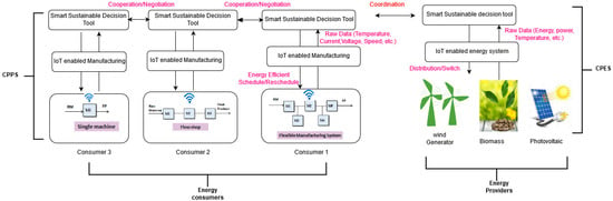
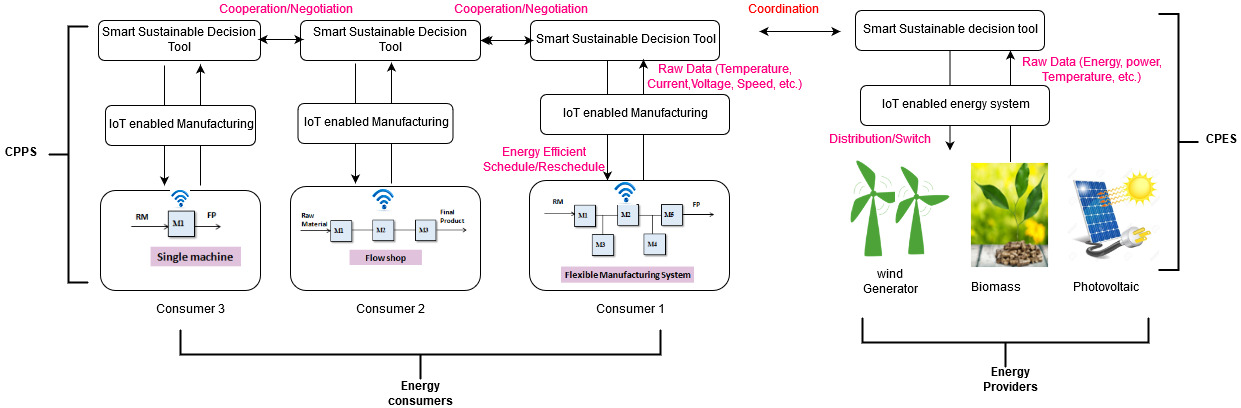
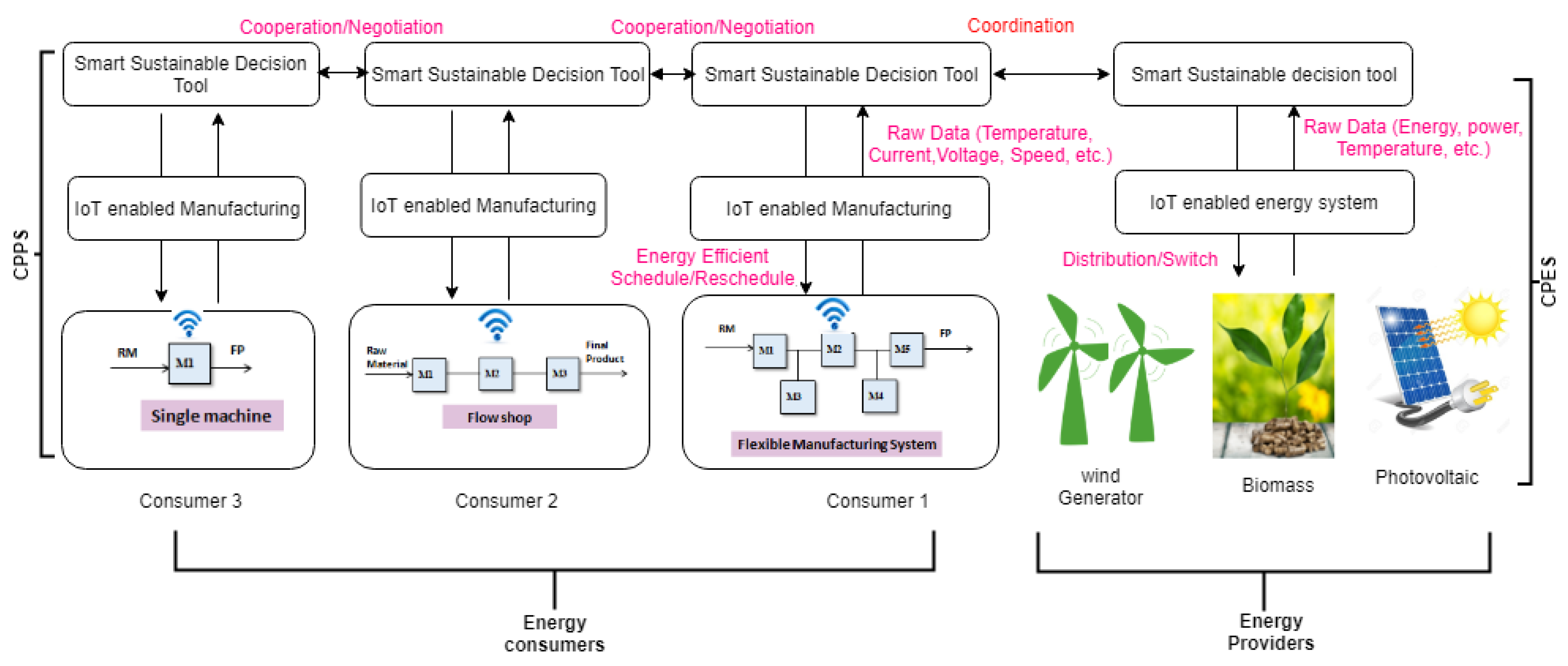
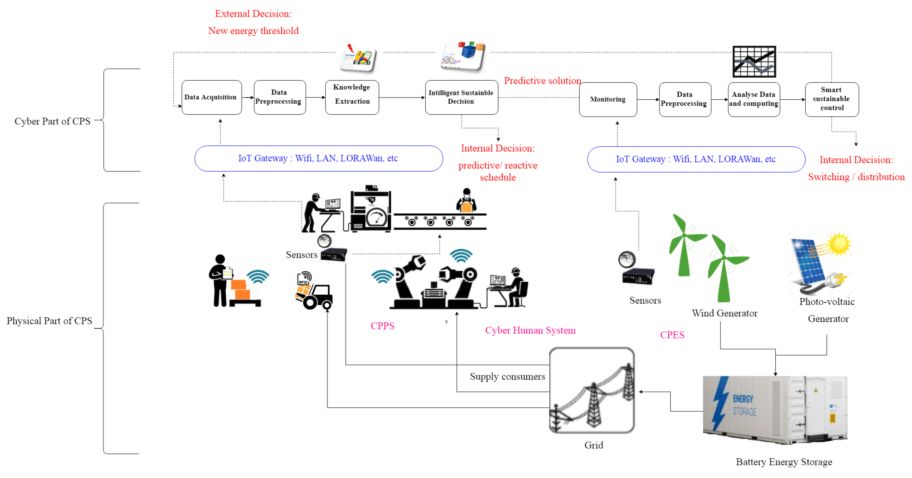
Our work, which relies on this context of sustainable development, exploits the concept of CPS and uses IoT technologies to deploy an energy-efficient distributed control architecture based on coordination between cyber physical production systems (CPPS) and cyber physical energy systems (CPES). As decentralized control is one of the main principles in industry 4.0 systems, in this work a multi-agent architecture, named EasySched, is proposed and implemented on a physically distributed architecture composed of embedded systems.
“The increasing volatility and unpredictability of energy availability, supply, and cost require the integration of highly reactive behaviour in control laws” [
13]. Thus, collaborative, predictive, and reactive mechanisms are proposed to provide energy efficient scheduling decisions. The mechanisms concern the calculation (predictive) and the adjustment (reactive) of the order of production of goods according to the availability of renewable energy.
Renewable energy production is difficult to predict because it is highly dependent on uncontrollable conditions (e.g., weather conditions). The data shared between CPS producing goods and CPS producing renewable energy is used to adjust scheduling decisions while ensuring sustainable goals. To illustrate this reactivity, developing a multi-agent system in a host (e.g., a personal computer) through a framework is insufficient. For this reason, the EasySched architecture was validated through multiple experiments on physically distributed systems. The innovative validation of this architecture was conducted in a comprehensive, physically distributed way, using networked embedded systems.
As first proof of concept, the factories and the energy providers were represented by embedded systems and sensors, respectively. The sensors were used to simulate energy perturbations and all the components were connected via a Local Area Network (LAN) network. To assess our proposal, the energy sources considered were wind and photovoltaic, the production systems were job-shops, and the energy consumption was adjusted by changing the speed of the production machines. Our approach dynamically adapts production in real time, and, therefore, energy consumption to energy supply. Note that this work is a proof of concept. When applied on a realistic case, some parameters should be adapted. A mathematical model is possible to confirm the results obtained by our approach and the Constraint Programming (CP) optimizer.
A literature review on cyber physical systemss and energy efficiency scheduling methods is presented in
Section 2. Details of the proposed architecture are given in
Section 3. The implementation of EasySched is detailed in
Section 4 and
Section 5 provides the results and the interpretations of the experiments. A conclusion and future prospects are described in
Section 6.
4. Implementation of EasySched
This section details the physical distributed systems used as an example to verify the feasibility of the proposed architecture and to asses the performance of EasySched. A physical distributed validation, on different systems, integrating the physical elements (hardware with connected sensors (IoT)) and the software is proposed in this article. These elements are connected via networks and cooperate to provide sustainable decisions. The real target system is the AIP-PRIMECA cell at the Polytechnic University Hauts-de-France. In the first experiment, the Acorn RISC Machine (ARM) embedded system was considered as a factory. The photovoltaic energy system was represented by the ARM embedded system with a luminosity sensor. The wind energy system was represented by the ARM embedded system with a temperature/humidity sensor.
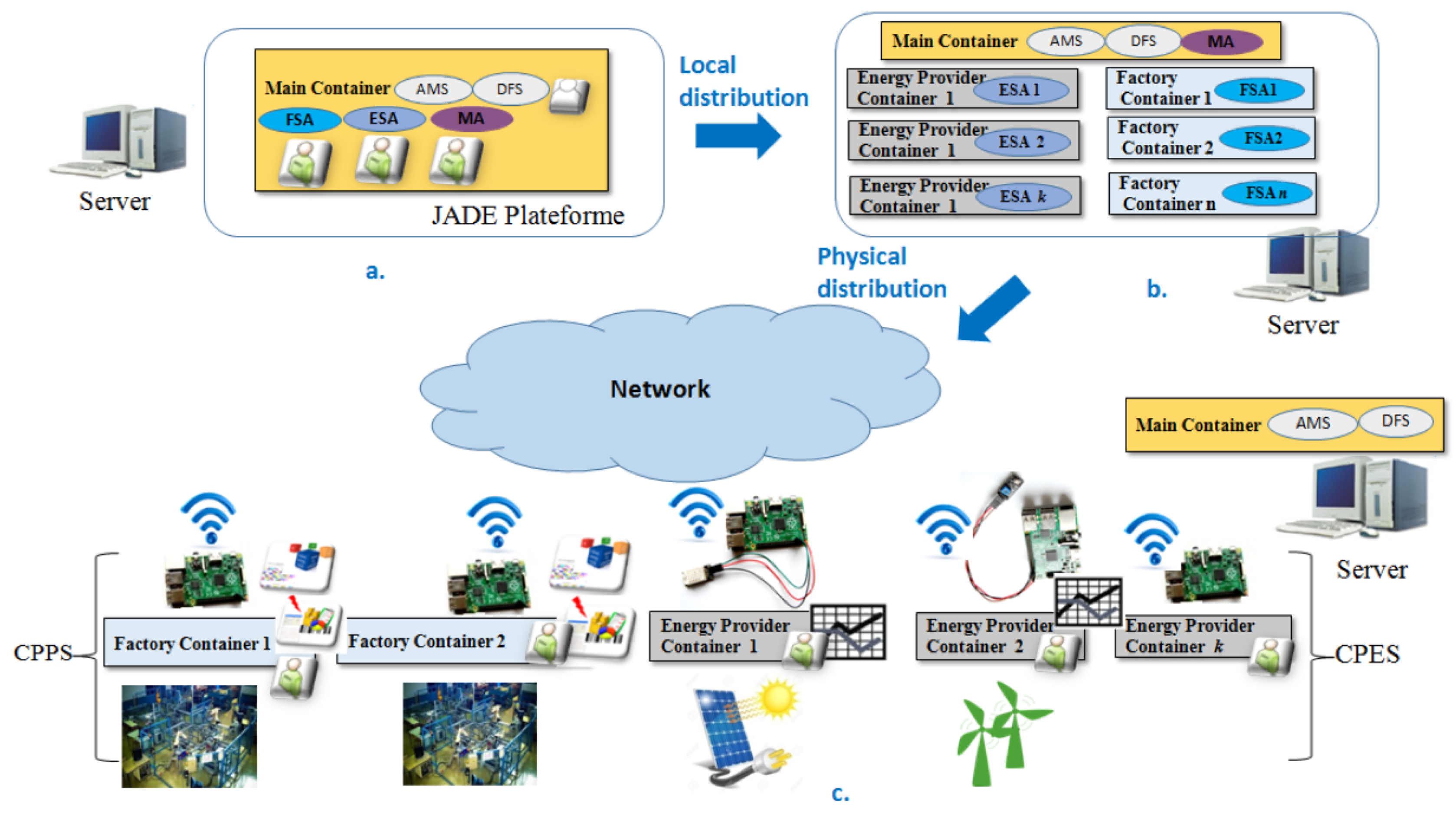
Figure 8 illustrates the implementation steps of the EasySched architecture composed of five ARM embedded systems.
The first step of the implementation was to propose agent behaviours of agents, negotiation, and coordinated mechanisms between agents and code them locally in the same main container (see
Figure 8a). In a multi agent context, an agent requires the presence of a container. A container is an abstract class that contains all the services needed to host and manage agents during the execution of their behaviours (software program). These agent containers can be distributed throughout the network. The agents created are by default located in the same “Main container”. Before being deployed to the physically distributed system comprising connected embedded systems, a container is created for each distant agent (see
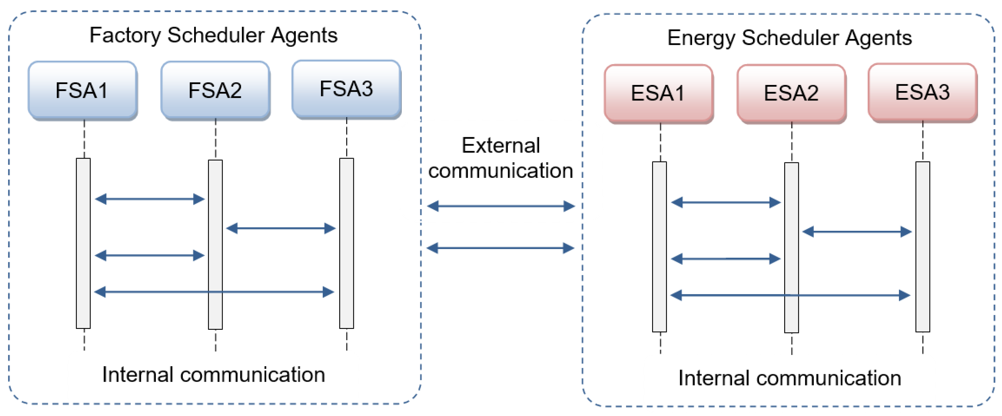
Figure 8b). “Factory Container i” and “Energy Provider Container i” are thus containers allocated to agents FSA and ESA respectively (see
Figure 8b). ARM A7 embedded systems are used to embed the ESA1, ESA2, FSA1, FSA2, and MA containers (see
Figure 8c).
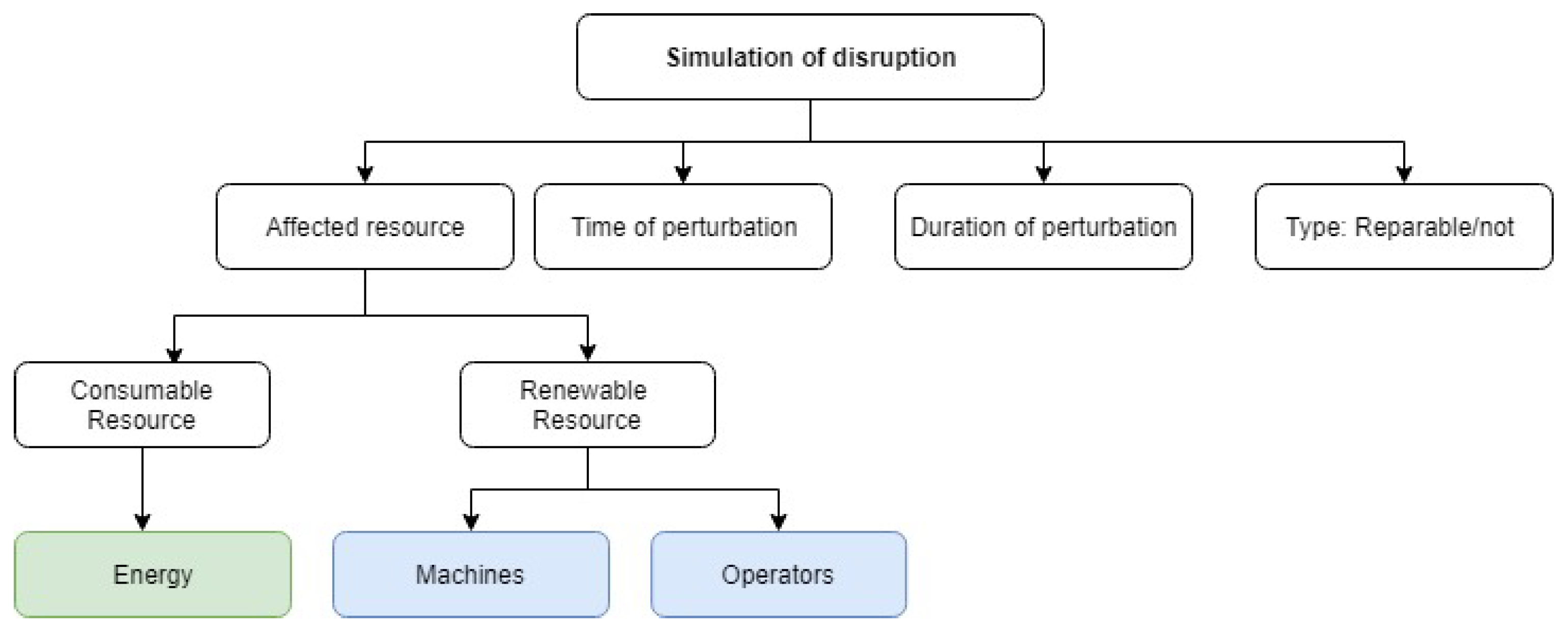
In order to validate the proposed dynamic mechanisms of the sustainable decision tools of CPPS and CPES, a set of perturbations is simulated. Luminosity, temperature, and humidity sensors are used to simulate the fluctuation of renewable energy. In our approach, the outputs of these sensors represented the variation in the quantities of certain parameters on which the power supplied by the two energy resources depends. For example, the variation in luminosity, which systematically influences the variation in the power delivered by any photovoltaic power generator is easily simulated by masking the light sensor to varying degrees. Similarly, the power delivered by a wind power generator depends on the temperature and humidity and can modified by influencing the temperature and humidity sensors.
The pseudo code that allows the ESA to detect a fluctuation in energy provided by a wind generator is detailed in Algorithm 5. In the context of this work, the model proposed by (Marshall and Plumb., 2008) was used, where the electric power delivered by a wind turbine can be calculated as follows:
where
S is the area of the wind turbine,
V is the wind speed, and
is the air density.
The air density is calculated as follows in Equation (
4):
where
T and
are the temperature and the humidity recovered from the sensors and the air pressure
p equals 1013.25 hPa. Powers
P(
t) and
P(0) are calculated using the previous equation. If the ratio
P(
t)/
P(0) is lower than 1, energy production decreases. The “Alarm” variable determining the system status is then updated.
| Algorithm 5 Pseudo code of ESA Monitoring behaviour |
- 1:
Read data from sensors (temperature and humidity in our case) - 2:
calculate the power P(t) - 3:
ifP(t)/P(0) < 1 then - 4:
Alarm = “Perturbation Detected” - 5:
else - 6:
Alarm = ”No perturbation” - 7:
end if
|
From a technical point of view, to limit the effect of sensor noise on the signals and thus avoid considering ever change in signal as a disturbance, an artificial filtering algorithm was added as data pre-processing behaviour. For this, the period of this cyclic behaviour was bigger than the data acquisition behaviour period.
The pseudo code for this cyclic behavior is represented in Algorithm 6.
| Algorithm 6 Pseudo code of ESA alarm triggering behaviour |
- 1:
if Alarm = “Perturbation detected” then - 2:
timeResch = timeResch + - 3:
Reschedule.timeResch = timeResch - 4:
Reschedule.tauxEnergy = (P(0) − P(t)/P(0)) × 100 - 5:
ControlMessage.Object = Reschedule - 6:
Send (ControlMessage, FSA) - 7:
- 8:
else - 9:
ControlMessage.State = “No energy perturbation” - 10:
Send(ControlMessage, FSA) - 11:
end if
|
In order to avoid successive launches of rescheduling signals, the period of cyclic behaviour is then modified when the ESA detects an anomaly (see line 7 in Algorithm 6).
5. Experimentation and Interpretation of Results
The distributed implementation consists of a PC and five ARM A7 embedded systems (FSA1, FSA2, ESA1, ESA2, and MA). The PC has an Intel Core i7 processor with 8 GB of RAM. The integrated card operates at 900 Mhz with 1 GB of RAM. The target embedded system runs the Debian version of Linux. All the machines run Java SE Embedded. A LAN is used for communication between all IoT components. The multi agent model was developed using the Java Agent Development Framework (JADE) multi agent platform in Netbeans IDE. To test the efficiency and the performance of the proposed EasySched architecture through its distributed implementation, different tests were performed on various types of job-shop benchmarks using machines with different speeds. Instances were named “machines_Vmax_Pi” where (machines) is the number of machines, (Vmax) is the maximum number of tasks per job and (Pi) is the range of processing times. For example, instance
refers to three machines with five operations per job and a processing time range of 10. Instance details are provided in [
43]. Each instance was executed five times. For our experiments, the periods
,
,
are initially set to 3 s, 6 s, and 8 s respectively.
x is set to 3.
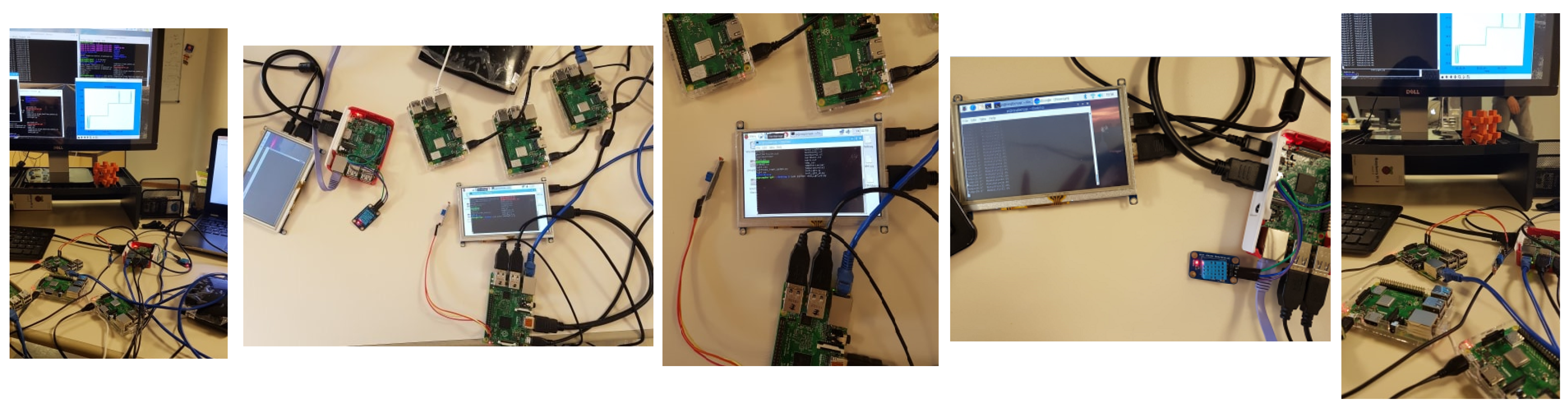
Figure 9 presents a selection of real photos of our distributed implementation in the LAMIH Laboratory. The experiment comprises two stages: The first one concerns the validation of the predictive part of EasySched and the second concerns the assessment of the reactive part. Relevant performance measurements are provided in the
Section 5.1.
5.1. Rescheduling Performance Measures
In order to asses the performance of the rescheduling method, performance indicators (KPI) had be defined. In fact, in order to compare the quality of the initial schedule (predictive) and the reactive one (after rescheduling), it is necessary to define two types of performance measurements depending on the evolution of the effectiveness or the efficiency [
42]. They are presented hereinafter.
Makespan Effectiveness: Proposed in [
56], it is defined as the percentage change in makespan of the predictive schedule compared to the original schedule.
where
is the makespan of the repaired schedule using the new proposed rescheduling methods and
is the makespan of the original schedule. The maximum efficiency 100% is achieved if the makespan of the predictive and the reactive schedule are identical. If the increase in the makespan when a disruption occurs is minimal, the rescheduling process is efficient.
Energy Efficiency: Is as a percentage change in energy consumed by the reactive schedule compared to the predictive one and is defined as follows:
where
and
represent respectively the reactive and the predictive energy consumption. Valuesgreater than 100%, mean that the energy consumption of the reactive one is lower than the predictive one. This is due to the energy constraint threshold that varies in real time depending on the fluctuation in renewable energy.
5.2. Experimentation and Results of Predictive Part
In this subsection, the results of the predictive part are presented and discussed. As explained previously, the objective of the ESA in the CPES is to validate the predictive solutions found by the FSA. To asses the efficiency of the PSO algorithm used by the FSA, it is compared with the CPLEX CP optimizer results of Salido et al. [
57]. CP optimizer was used as a reference to evaluate the efficiency and performance of our approach.
Table 2 contains the results of the tests. The first column represents the names of the instances, following columns present the Makespan (Mk, in seconds) and the energy consumed (E in Wh) provided by the FSA1 and FSA2. The weighting parameter
and the control message sent by the ESA are also specified. “Yes” refers to the approval of the predictive schedules, whereas “No” triggers the FSA to find another solution after negotiating with other FSAs while reducing the weighting parameter
. The last columns represents Mk and E found by the CP Optimizer in [
57]. As it can be seen, the PSO results are efficient in terms of the quality of the solutions found. The Mk values are the same for small instances compared with the CP Optimizer. The Mk and E are very close to the CP optimizer values. The total average deviation between the results of FSA1 and the CP Optimizer is 2.8% for makespan and 0.6% for energy consumption. More details are described in
Appendix A.
These predictive experiments also aim to validate the negotiation protocol between agents (FSA and ESA) presented in Algorithm 3. The search for the predictive solution is repeated until the approval message “yes” is received from the ESA indicating that the CPES has sufficient energy to satisfy demands.
As one can see from
Table 2, the ESA sends approval messages only if the sum of the energy demand is lower than or equals to a fixed predictive energy threshold. For instance 1, the ESA sends a “Yes” message when the energy is lower than 5000 in instance 2, etc. These results validate the effectiveness of the negotiation protocol between factory schedulers and energy schedulers.
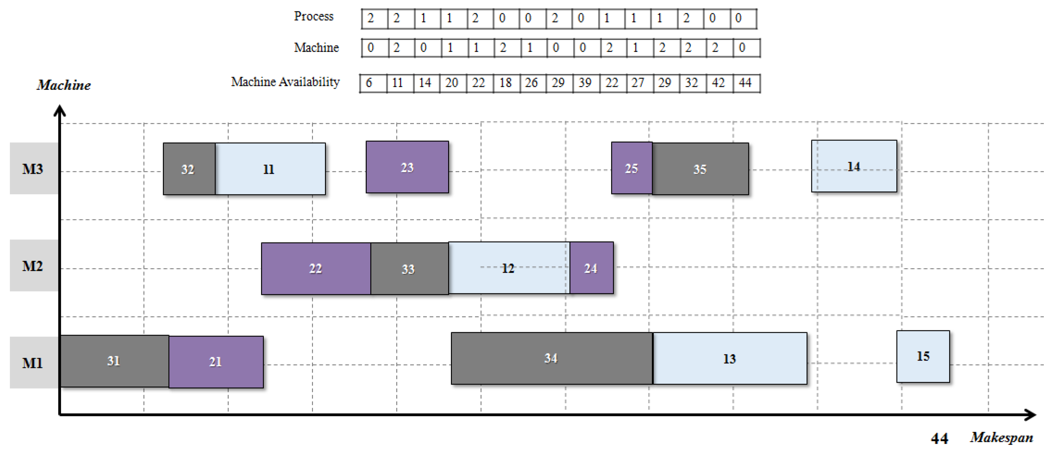
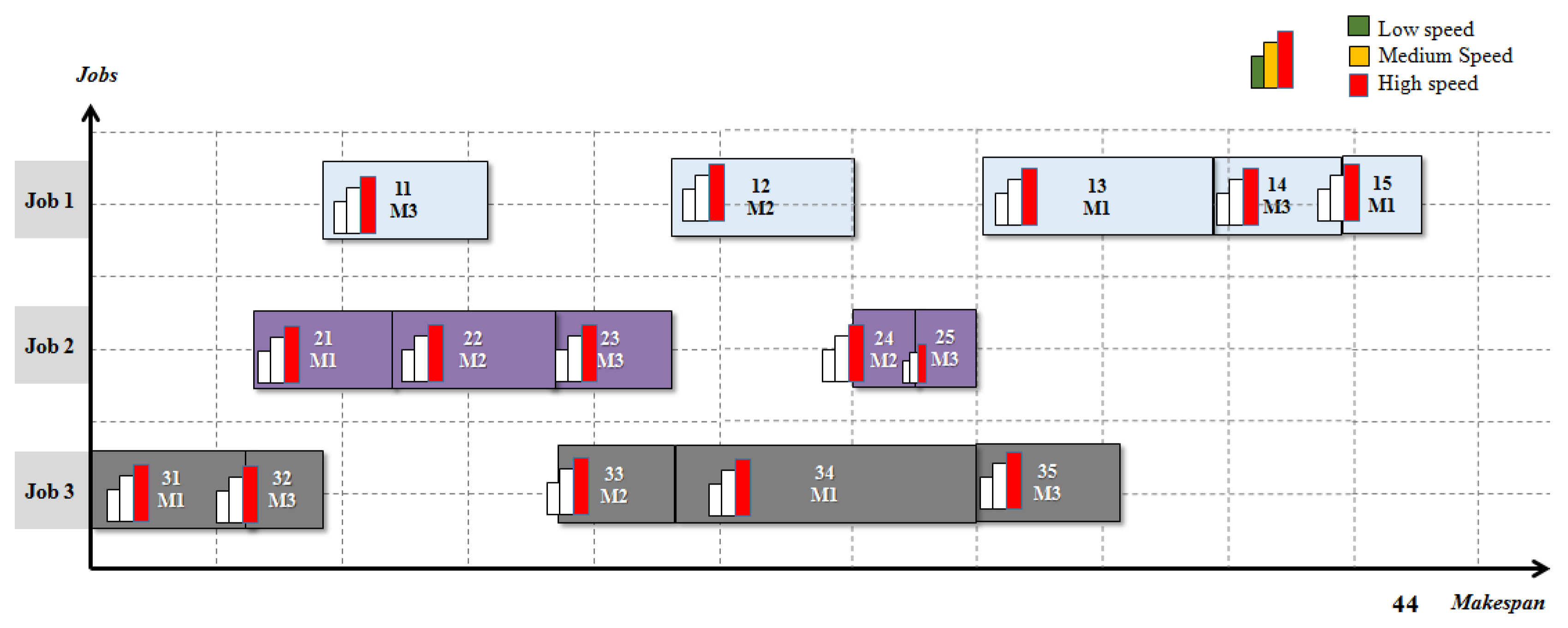
Figure 10 illustrates the predictive solution delivered by FSA 1 after executing the PSO algorithm. The makespan of this solution equals 44 s and the energy consumption is 133 Wh. The particle (the PSO algorithm output) corresponding to this solution and the Gantt chart are given in
Figure 10. The machine availability vector in the particle representation is useful to extract the affected operations in case of disruption and to follow its propagation (see
Figure 10).
Figure 11 illustrates the profiling of machine speed used in the predictive solution. As we can see, in this solution the machines are used in high speed to favor the reduction of the completion time.
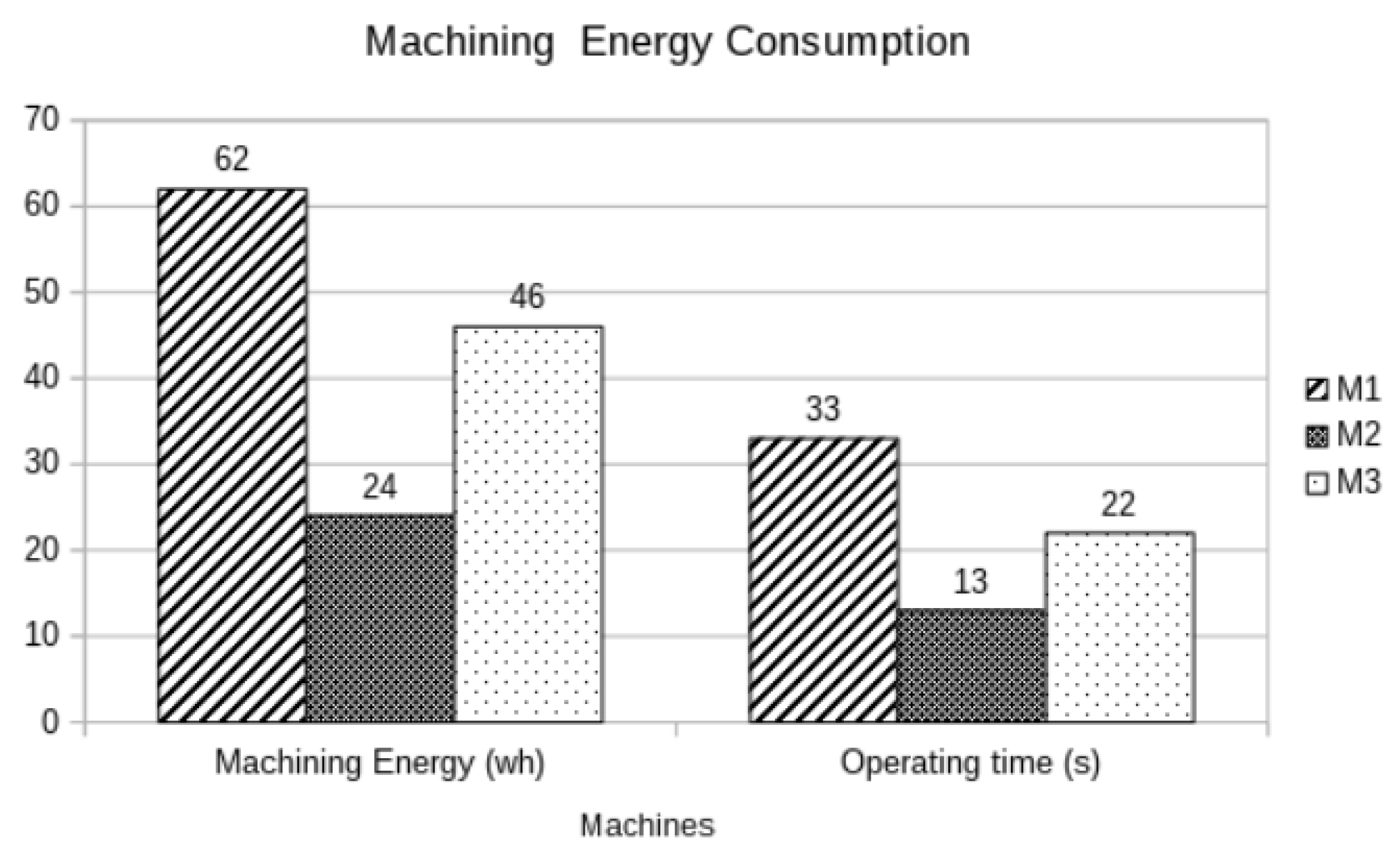
Figure 12 illustrates the profiling of the energy consumption per machine with the predictive solution. The idle energy consumption, that refers to the consumption during the slack times, is not calculated in this work because the power of the machines is not specified in the instances in [
43]. However, it remains a very important characteristic that affects the total energy consumption.
5.3. Experimentation and Results of the Reactive Part
The objective of the experimentation is to validate the reactive part of the proposed architecture. For this purpose, many perturbations were simulated to affect the predictive solutions. As mentioned before, the fluctuation of the renewable energy is simulated by varying the output of the luminosity, temperature and humidity sensors.
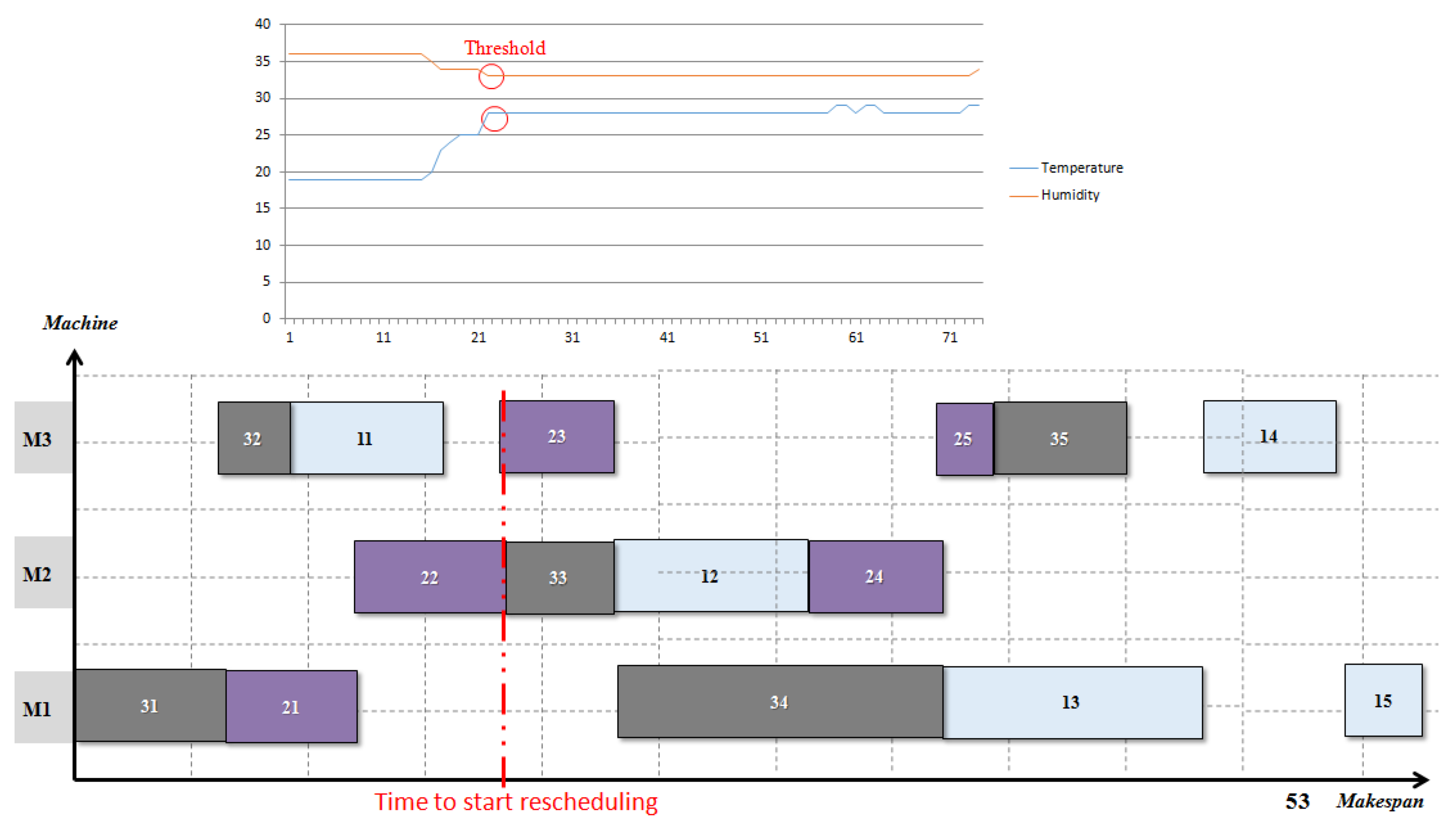
Figure 13 illustrates the sensing data results acquired by the ESA after executing the monitoring behaviour. The analysis of the data enables any fluctuations in renewable energy to be detected. As in the predictive part the makespan (Mk) and the energy consumption (EC), which reflect production and energy efficiency respectively are estimated.
Table 3 summarizes the results of the reactive experiments when faced with energy perturbations. The makespan and the energy consumption of predictive and reactive solutions are compared.
Table 3 contains the Mk and EC of the predictive and reactive solutions respectively while specifying the energy threshold communicated by the ESA that controls this factory. It compares the performance of the reactive solutions found by the rescheduling methods with the predictive solutions. As one can see, in most cases, the FSA was able to find a new solution respecting the energy constraint.
Figure 14 contains the Gantt diagram of a reactive schedule found by the factory scheduler agent FSA1 after executing the rescheduling method. As we can see from this figure, a new energy threshold was detected and communicated by the CPES. This trigger launches the rescheduling procedure at time 22 s (trigger time). The energy consumption of the reactive schedule found was reduced to 94 Wh after the disruption while the makespan is degraded to 53 s (see
Figure 14). As we can see, the energy consumption and the makespan of the predictive and the reactive schedules are not the same. However, there is a small deviation in Mk value from 44 s to 53 s and in EC value from 133 Wh to 94 Wh. The new energy consumption of the reactive schedule respected the energy threshold 26%.
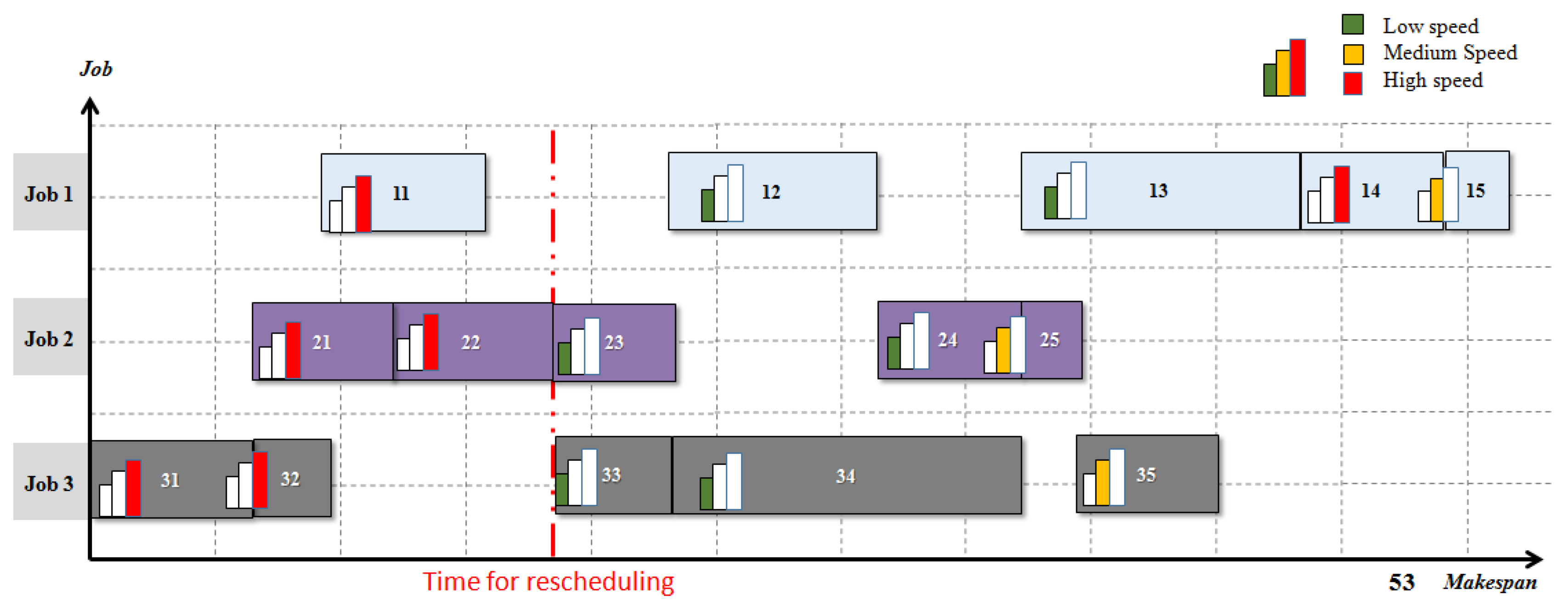
Figure 15 illustrates the variation of the speed of machines of the affected operations to reduce the energy consumption. The high machine speeds were reduced to low and medium speed. In this scenario, the adaptation of the energy consumption of the factory to respect the 26% energy threshold led to a deterioration in the makespan performance (an increase in the production completion time). However, the quantification of this degradation depends on the production and energy consumption models used. This solution was found using the first rescheduling method proposed that seeks to preserve stability and change the speeds of machines to meet the energy constraint. The speeds of the machines M1, M2, and M3 are thus changed starting from the rescheduling time (see
Figure 15).
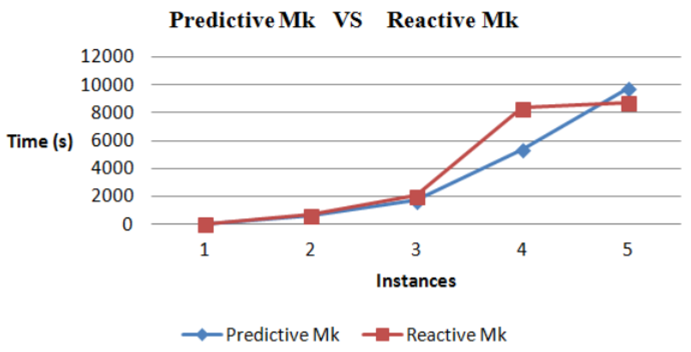
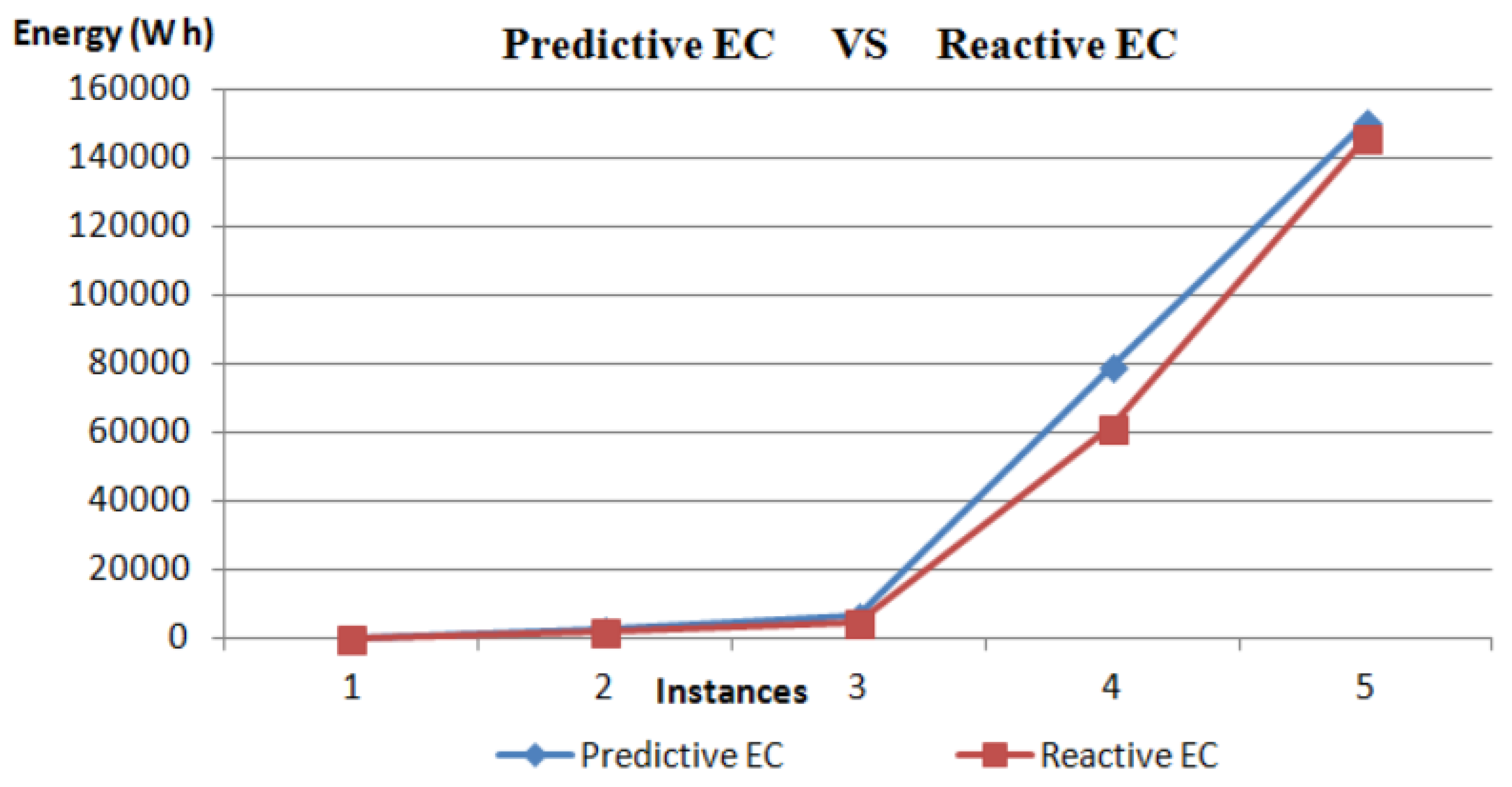
Figure 16 and
Figure 17 show the deviation between the predictive and reactive makespan and energy consumption respectively. The results obtained validate the efficiency and the reactivity of the proposed multi agent architecture.
Table 4 presents the makespan efficiency and the energy efficiency for the different instances. For instance 1, Makespan Efficiency (ME) equals 79%, which means that the makespan has not degraded much compared to the predictive makespan. However, Energy Efficiency (EE) equals 129%, which means a decrease in EC with regards to the energy threshold. Thus, the reactive energy value is lower than the predictive one.
Even though the results seem to be in favour of the proposed EasySched, the simulation results obtained for all the cases were examined using an analysis of variance (one way ANOVA) to conclude if there was a statistically significant difference to support our conclusions. A statistical sensitivity test has been performed on the results.
In order to validate the obtained results, an ANOVA analysis is performed. The results obtained with the one-way ANOVA are presented in
Table 5. The F-ratio and the
p-value show the impact of the perturbation on the quality of the predictive solution.
The impact is considered significant for
p-values < 0.05. However, according to the
p-values in
Table 5, the perturbation does not have a significant impact.
The results presented above represent the first implementation case where each CPPS was connected to a different CPES (factory 1 to wind generator, factory 2 to photovoltaic generator). In the next subsection, the results of the second situation are analysed.
5.4. Self Configuration of CPES
Contrary to the configuration in the previous section, the results presented in this section were obtained from the second implementation case of EasySched where all CPPSs were connected to the same CPES.
Table 6 and
Table 7 summarize the results of the experiments related to the dynamic configuration of the weighting parameter to switch between energy sources. Some assumptions are taken into consideration. Firstly, all renewable energy generators (represented by CPES) were combined and controlled by a global ESA delegated to make decisions to control the distribution of energy portion from each generator autonomously. As the luminosity sensor used in our experiments was digital and not analogue, the output was binary (0 or 1) and therefore, we could not quantify the power delivered by the photovoltaic generator. However, in this case, the weighting parameter
was set to 0.5 when the output (sensor data) was 1 or 0.2 otherwise. If there is a decrease in wind energy,
is decreased. If there is a power degradation by 10% for example
is reduced by 0.1, for 20%
is reduced by 0.2, etc.
As we can see from this experiment, the ESA was able to provide internal intelligent decisions to self-configure the weighting parameter responsible for switching the energy supply depending on the fluctuation in the power of each renewable energy generator.
Other scenarios can be imagined in the context of switching between energy sources, for example, the dynamical real-time variation in the price could also be treated as a source of perturbation.
5.5. Discussion
The results obtained by EasySched architecture seem to be promising in terms of makespan and energy efficiency of the obtained solutions. The architecture enables the connected factories to adjust especially their consumption in terms of an energy threshold communicated in real-time by CPES. A statistical sensitivity test has been performed on the results. However, formal studies have to be conducted to prove the effectiveness and efficiency in predictive and reactive parts. Other self configuration mechanisms have to be designed for the CPES to switch between different renewable sources.


