Design of Disturbance Extended State Observer (D-ESO)-Based Constrained Full-State Model Predictive Controller for the Integrated Turbo-Shaft Engine/Rotor System

Abstract

In the modern helicopter design and development process, constrained full-state control technology for turbo-shaft engine/rotor systems has always been a research hotspot in academia and industry. However, relevant references have pointed out that the traditional design method with an overly complex structure (Min-Max structure and schedule-based transient controller, i.e., M-M-STC) may not be able to meet the protection requirements of engine control systems under certain circumstances and can be too conservative under other conditions. In order to address the engine limit protection problem more efficiently, a constrained full-state model predictive controller (MPC) has been designed in this paper by incorporating a linear parameter varying (LPV) predictive model. Meanwhile, disturbance extended state observer (D-ESO) (which a sufficient convergence condition is deduced for) has also been proposed as the compensator of the LPV model to alleviate the MPC model mismatch problem. Finally, we run a group of comparison simulations with the traditional M-M-STC method to verify the effectiveness of this controller by taking compressor surge prevention problems as a case study, and the results indicate the validity of the proposed method.

1. Introduction

In current years, with the development of aircraft engine technology [1,2,3,4], the complexity of engine working conditions is increasing. Accordingly, the engine controller is getting more and more critical to engine transitions from one state to another, while preventing the engine from dropping into abnormal conditions, such as over-speed, over-temperature, stall, surge, etc. Therefore, how to design a constrained full-state controller (including steady-state control, transient control, and limit protection control) is of great significance in both theory and practice. It is particularly important and necessary for an integrated turbo-shaft engine/rotor control system (see Figure 1) as an excellent control algorithm allows a larger operation range for rotors [5,6]. Hence, in this paper, a versatile full-state control strategy specifically established for a class of turbo-shaft engine/rotor system is proposed, which can take into account all performance constraints of transient state control.

At present, the common design methods for the constrained full-state control are schedule-based [7,8] (accelerating and decelerating program) or based on N-dot transient control law [8,9] (direct N-dot and indirect N-dot). Generally, both methods can only work by binding to the Min-Max structure and the linear controller [10]. In the meantime, relevant references point out that these traditional methods are confronted with problems as follows [10]: (1) It is not always accurate enough to provide limit protection for the engine; (2) The obtaining of acceleration or deceleration plans of the schedule-based approach requires large number of testings, which are time-consuming and money-consuming; (3) Min-Max selection logic structure will make the control system complex; (4) They are too conservative to run the engine under optimal performance.

Considering the drawbacks of the traditional transient control methods, various kinds of advanced algorithms have been proposed, such as sliding mode control [11], adaptive control [12], and model predictive control (MPC) [13,14]. Among them, MPC’s prediction ability as well as its capability of coping with constrained optimization problems without Min-Max structure has widely interested researchers. Since the 1990s, significant developments in theory and application for MPC have been achieved, such as dynamic matrix control [15], generalized predictive control [16], etc. In the field of aero-engines, MPC also comes into use to solve some limit protection problems of transient control [10,11,12,13,14,15,16,17]. In the book [10], the standard state-space formulation of MPC for linear plants was presented. In [17], Morteza made a comparison of MPC and the Min-Max algorithm for a turbofan engine. However, even though the MPC controller mentioned in these references can conquer the conservation problem of traditional methods to some degree, it ignored two crucial points of the MPC algorithm: heavy computational burden and model mismatch phenomenon.

As for a nonlinear system, heavy computational burden [18,19] always introduces difficulties into the MPC design process. Chen in [19] took the computational delay into account, and proposed a modified MPC controller. However, [20] pointed out that the method in [19] may render the optimization problem infeasible. Although the linear matrix inequation (LMI) method mentioned in the robust MPC algorithm [21] can also reduce the computational burden, the feasibility problem is still a major problem for LMI technique. The linear MPC method can reduce the on-line computational burden, however, it can cause the model mismatch phenomenon at the same time. Linear parameter varying (LPV) systems are always established from a set of linear time invariant systems obtained by a linearization process near some equilibrium states of the nonlinear systems, which inevitably leads to the linearization error. Thus, spontaneously, the model mismatch problem arises [22].

For the nonlinear turbo-shaft engine/rotor system in this paper, we develop a LPV-based MPC controller to reduce the computing load. Meanwhile, considering the model mismatch phenomenon, a disturbance extended state observer (D-ESO) is designed to compensate the linearization error between LPV and a real turbo-shaft engine/rotor system. D-ESO has achieved significant progress in dealing with systems with parameter uncertainty [23], great time lag [24], and external disturbances [25]. Unlike general observer, D-ESO can be utilized not only to observe the system states but also to handle disturbances by being treated as extended states [26]. In this regard, its effectiveness has been proved by relevant literature [27]. Inspired by this property of D-ESO, by treating the error between the LPV model and the real turbo-shaft engine/rotor as the disturbance, it makes possible for a D-ESO to solve the model mismatch problem arising from the LPV model before the controller design.

In this paper, we present a new D-ESO-based MPC controller design method to achieve constrained full-state control of turbo-shaft engine/rotor systems. Firstly, the LPV system is described based on a turbo-shaft engine/rotor nonlinear system. After that, D-ESO is proposed to solve the model mismatch problem of the predictive model in MPC. The sufficient conditions of convergence of D-ESO are also discussed in Theory 1. Meanwhile, its effectiveness of which is verified, i.e., a group of simulation results show that D-ESO is efficient for overcoming the model mismatch problem of linear predictive model, which means more accurate engine behavior prediction. Secondly, on the basis of the D-ESO and LPV model, a constrained full-state MPC controller for turbo-shaft engine/rotor system is developed. Finally, a group of simulations are applied to the surge prevention for integrated turbo-shaft engine/rotor system. The simulation results reveal that the D-ESO-based MPC controller law proposed here can not only perform well during full-state process, but also guarantee all the limit parameters value within the limited range. Moreover, through the comparison test with the Min-Max structure and schedule-based transient controller (M-M-STC), the effectiveness of the methods in this paper is further confirmed.

The contributions of this paper lie in the following aspects:

• The D-ESO method can overcome the mismatch problem of the predictive model.
• For the LPV system, we give a sufficient condition for the convergence of the D-ESO in Theory 1.
• In comparison with the nonlinear MPC case, MPC based on the LPV model and the D-ESO method in this paper has the advantage of minor calculation.
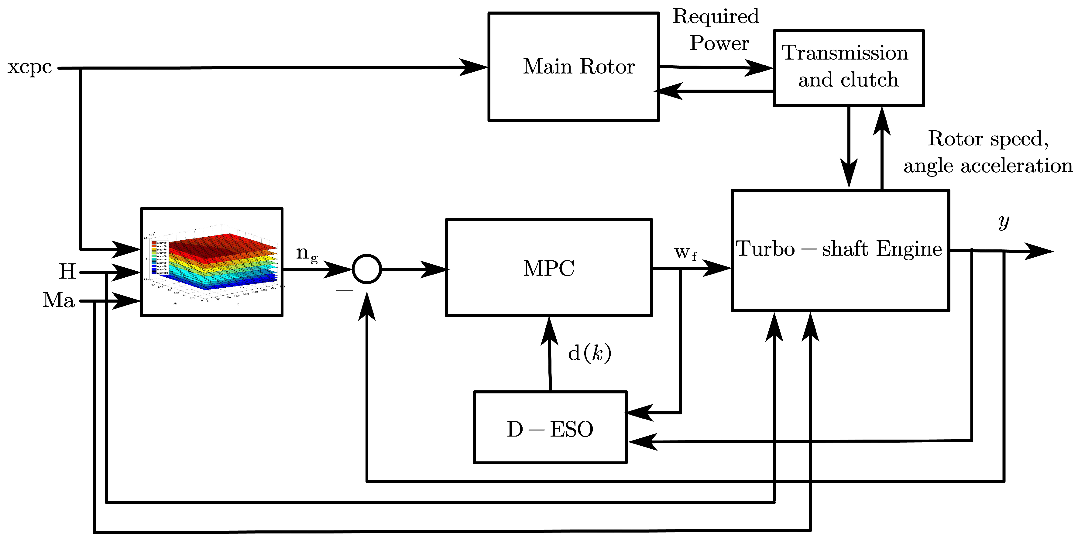
• A new D-ESO-based MPC controller is designed in this paper to achieve the constrained full-state control of the turbo-shaft engine/rotor system. Compared with M-M-STC strategy, it can not only conquer the high cost and conservation problem of traditional methods, but also leave out the complex structure of Min-Max selection logic strategy.

2. Predictive Model-LPV System

Aiming at a component level aerothermodynamic model of integrated turbo-shaft engine/rotor system (Figure 2), MPC controller strategy is presented to realize its constrained full-state control. The structure of the engine/rotor system can be described in general as a nonlinear continuous time ordinary differential equation using the following equation:

$$\begin{array}{cc}\hfill \left[\begin{array}{c}\dot{{\mathrm{n}}_{\mathrm{g}}},\dot{{\mathrm{n}}_{\mathrm{p}}}\end{array}\right]& =f\left({\mathrm{n}}_{\mathrm{g}},{\mathrm{n}}_{\mathrm{p}},{\mathrm{w}}_{\mathrm{f}},\mathrm{xcpc}\right)\hfill \\ \hfill \left[\begin{array}{c}{\mathrm{Out}}_{\mathrm{t}},{\mathrm{Out}}_{\mathrm{l}}\end{array}\right]& =h\left({\mathrm{n}}_{\mathrm{g}},{\mathrm{n}}_{\mathrm{p}},{\mathrm{w}}_{\mathrm{f}},\mathrm{xcpc}\right)\hfill \end{array}$$

(1)

where ${\mathrm{n}}_{\mathrm{g}}$ and ${\mathrm{n}}_{\mathrm{p}}$ are the gas turbine and power turbine speeds respectively. ${\mathrm{Out}}_{\mathrm{t}}$ is the tracking signal selected by us, ${\mathrm{Out}}_{\mathrm{l}}$ represents a group of limit parameters that need to be taken into account during the controller design process, ${\mathrm{w}}_{\mathrm{f}}$ represents the fuel flow, and $\mathrm{xcpc}$ is the collective pitch input of rotor system.

However, the explicit formula in Equation (1) is difficult to obtain from the above component level model (see Figure 2) and cannot be used as the predictive model of MPC for the reason of nonlinearity, and thus heavy computational burden. Therefore, we design the MPC controller with the aid of a discrete LPV system.

$$\begin{array}{cc}\hfill x\left(k+1\right)& =A\left(\alpha \left(k\right)\right)x\left(k\right)+B\left(\alpha \left(k\right)\right)u\left(k\right)+B_w\left(\alpha \left(k\right)\right)w\left(k\right)\hfill \\ \hfill y_t\left(k\right)& =C_t\left(\alpha \left(k\right)\right)x\left(k\right)+D_t\left(\alpha \left(k\right)\right)u\left(k\right)+D_{wt}\left(\alpha \left(k\right)\right)w\left(k\right)\hfill \\ \hfill y_l\left(k\right)& =C_l\left(\alpha \left(k\right)\right)x\left(k\right)+D_l\left(\alpha \left(k\right)\right)u\left(k\right)+D_{wl}\left(\alpha \left(k\right)\right)w\left(k\right)\hfill \end{array}$$

(2)

where $x=\left[\begin{array}{c}{\mathrm{n}}_{\mathrm{g}}-{\mathrm{n}}_{\mathrm{g}0}\\ {\mathrm{n}}_{\mathrm{p}}-{\mathrm{n}}_{\mathrm{p}0}\end{array}\right]$, $u\left(k\right)={\mathrm{w}}_{\mathrm{f}}-{\mathrm{w}}_0$, ${\mathrm{y}}_t={\mathrm{Out}}_{\mathrm{t}}-{\mathrm{Out}}_{\mathrm{t}0}$, ${\mathrm{y}}_l={\mathrm{Out}}_{\mathrm{l}}-{\mathrm{Out}}_{\mathrm{l}0}$, $w\left(k\right)=\mathrm{xcpc}-\mathrm{xcp}{\mathrm{c}}_0$, and ${\mathrm{n}}_{\mathrm{g}0}$, ${\mathrm{n}}_{\mathrm{p}0}$, ${\mathrm{w}}_{\mathrm{f}0}$, $\mathrm{xcp}{\mathrm{c}}_0$, ${\mathrm{Out}}_{\mathrm{l}0}$, and ${\mathrm{Out}}_{\mathrm{t}0}$ are the equilibrium points value of the corresponding parameters. For convenience in writing, $\alpha \left(k\right)$ will be abbreviated to $\alpha$ below and in later content.

The coefficients of Equation (2) $A\left(\alpha \right)$, $B\left(\alpha \right)$, $B_w\left(\alpha \right)$, $C_t\left(\alpha \right)$, $D_t\left(\alpha \right)$, $D_{wt}\left(\alpha \right)$, $C_l\left(\alpha \right)$, $D_l\left(\alpha \right)$, and $D_{wl}\left(\alpha \right)$ belong to one convex polytope $\Omega$,

$$\left[\begin{array}{c}A,B,B_w,C_t,D_t,D_{wt},C_l,D_l,D_{wl}\end{array}\right]\left(\alpha \right)\in \Omega .$$

(3)

The set $\Omega$ is of the following polytope type,

$$\Omega =C_O\left\{\begin{array}{c}\left[\begin{array}{ccccccccc}{A}_1& B_1& B_{w1}& C_{t1}& D_{t1}& D_{wt1}& C_{l1}& D_{l1}& D_{wl1}\end{array}\right],\hfill \\ \cdots ,\left[\begin{array}{ccccccccc}{A}_L& B_L& B_{wL}& C_{tL}& D_{tL}& D_{wtL}& C_{lL}& D_{lL}& D_{wlL}\end{array}\right]\hfill \end{array}\right\}$$

(4)

where, $C_O$ devotes to the convex hull and $A_i\in R^{2\times 2}$, $B_i\in R^{2\times 1}$, $B_{wi}\in R^{2\times 1}$, $C_{ti}\in R^{m_t\times 2}$, $D_{ti}\in R^{m_t\times 1}$, $D_{wti}\in R^{m_t\times 1}$, $C_{li}\in R^{m_l\times 2}$, $D_{li}\in R^{m_l\times 1}$, $D_{wli}\in R^{m_l\times 1}$, and $i=1,\cdots ,L$ are matrices obtained by linearizing the nonlinear model in Equation (1) with the small deviation linearization method.

Moreover, if $\left[\begin{array}{c}A,B,B_w,C_t,D_t,D_{wt},C_l,D_l,D_{wl}\end{array}\right]\left(\alpha \right)\in \Omega$, then there exist some nonnegative ${\lambda }_1,{\lambda }_2,\cdots ,{\lambda }_L$ such that,

$$\begin{array}{c}\hfill \left[A,B,B_w,C_t,D_t,D_{wt},C_l,D_l,D_{wl}\right]\left(\alpha \right)=\sum _{i=1}^L{\lambda }_i\left[A_i,B_i,B_{wi},C_{ti},D_{ti},D_{wti},C_{li},D_{li},D_{wli}\right]\end{array}$$

(5)

$$\sum _{i=1}^L{\lambda }_i=1.$$

(6)

3. Disturbance Based Extended State Observer (D-ESO)

Although, the LPV model (2) described above can capture the dynamic characteristic of the integrated turbo-shaft engine/rotor system, it inevitably introduces large errors compared to system (1) because of linearization. Considering the errors produced, the disturbance term $\mathrm{d}\left(k\right)$ is introduced into the state channel of system (2) to represent the errors, shown as follows,

$$\begin{array}{cc}\hfill x\left(k+1\right)& =A\left(\alpha \right)x\left(k\right)+B\left(\alpha \right)u\left(k\right)+B_w\left(\alpha \right)w\left(k\right)+\mathrm{d}\left(k\right)\hfill \\ \hfill y_t\left(k\right)& =C_t\left(\alpha \right)x\left(k\right)+D_t\left(\alpha \right)u\left(k\right)+D_{wt}\left(\alpha \right)w\left(k\right)\hfill \\ \hfill y_l\left(k\right)& =C_l\left(\alpha \right)x\left(k\right)+D_l\left(\alpha \right)u\left(k\right)+D_{wl}\left(\alpha \right)w\left(k\right)\hfill \end{array}$$

(7)

where $\mathrm{d}\left(k\right)=\left[\begin{array}{c}{\mathrm{d}}_1\left(k\right)\\ {\mathrm{d}}_2\left(k\right)\end{array}\right]$.

After adding the disturbance term $\mathrm{d}\left(k\right)$ in the LPV system, the D-ESO will be used below to observe the value of $\mathrm{d}\left(k\right)$, instead of observing the system states. The input-output relations of the turbo-shaft engine/rotor system, predictive model-LPV model, and D-ESO can be seen in Figure 3.

The main task following is to design an ESO observer to capture the linearization error $\mathrm{d}\left(k\right)$ in Equation (7) and use this observed error term to compensate LPV model such that predictive model mismatch problem can be overcome (see Figure 4 for the principal working principle of D-ESO).

3.1. D-ESO Design

The D-ESO designed for LPV system in Equation (7) is as follows:

$$\begin{array}{cc}\hfill e_1\left(k\right)& =z_1\left(k\right)-x\left(k\right)\hfill \\ \hfill z_1\left(k+1\right)& =A\left(\alpha \right)x\left(k\right)+B\left(\alpha \right)u\left(k\right)+B_w\left(\alpha \right)w\left(k\right)+z_2\left(k\right)-{\beta }_0{e}_1\left(k\right)\hfill \\ \hfill z_2\left(k+1\right)& =z_2\left(k\right)-{\beta }_1{e}_1\left(k\right)\hfill \end{array}$$

(8)

where $z_1\left(k\right)$, $z_2\left(k\right)$ are the estimated values of $x\left(k\right)$, $\mathrm{d}\left(k\right)$ respectively. ${\beta }_0=\left[\begin{array}{cc}{\beta }_{01}& 0\\ 0& {\beta }_{02}\end{array}\right]$, ${\beta }_1=\left[\begin{array}{cc}{\beta }_{11}& 0\\ 0& {\beta }_{12}\end{array}\right]$ and ${\beta }_{01}$, ${\beta }_{02}$, ${\beta }_{11}$, ${\beta }_{12}$ are positive adjustable parameters.

Before the discrete D-ESO being designed, it is assumed that,

Assumption A1.

For any arbitrary small sampling time T,

$$\begin{array}{c}\hfill {\Delta \mathrm{d}}_1\left(k\right)={\mathrm{d}}_1\left(k+1\right)-{\mathrm{d}}_1\left(k\right)\in o\left(T^2\right)\\ \hfill \Delta {\mathrm{d}}_2\left(k\right)={\mathrm{d}}_2\left(k+1\right)-{\mathrm{d}}_2\left(k\right)\in o\left(T^2\right)\end{array}$$

(9)

and the following relation is true,

$$o\left(T^n\right)+o\left(T^{n+1}\right)\approx o\left(T^n\right).$$

(10)

However, only when the convergence of D-ESO is guaranteed can the following relations hold: $z_1\left(k\right)\to x\left(k\right)$ and $z_2\left(k\right)\to \mathrm{d}\left(k\right)$. Therefore, in the following section, we will prove the sufficient conditions for the convergence of D-ESO in the form of theorem.

3.2. D-ESO Convergence Condition

Theorem 1.

Based on Assumption A1, for $\forall \left[\begin{array}{c}A\left(\alpha \right),B\left(\alpha \right),B_w\left(\alpha \right)\end{array}\right]\in \Omega$, if there exist positive real numbers ${\beta }_{01}$, ${\beta }_{02}$, ${\beta }_{11}$, ${\beta }_{12}$ such that

$$\begin{array}{cc}\hfill {\beta }_{11}-{\beta }_{01}& <0\hfill \\ \hfill 2-2{\beta }_{01}+{\beta }_{11}& >0\hfill \end{array}$$

(11)

$$\begin{array}{cc}\hfill {\beta }_{12}-{\beta }_{02}& <0\hfill \\ \hfill 2-2{\beta }_{02}+{\beta }_{12}& >0\hfill \end{array}$$

(12)

then D-ESO as defined in Equation (8) is convergent, that is: when $k\to \infty$, $z_1\left(k\right)\to x\left(k\right)$, $z_2\left(k\right)\to \mathrm{d}\left(k\right)$.

Proof 

For the convenience of derivation, we firstly try to transform system (7) into a particular form by linear transformation:

$$\overline{x}\left(k\right)=P\times x\left(k\right)=\left[\begin{array}{c}\overline{x_1}\left(k\right)\\ \overline{x_2}\left(k\right)\end{array}\right]$$

$$\begin{array}{cc}\hfill \overline{x}\left(k+1\right)& =\overline{A}\left(\alpha \right)\overline{x}\left(k\right)+\overline{B}\left(\alpha \right)u\left(k\right)+\overline{B_w}\left(\alpha \right)w\left(k\right)+\overline{\mathrm{d}}\left(k\right)\hfill \\ \hfill \overline{y_t}\left(k\right)& =\overline{C_t}\left(\alpha \right)\overline{x}\left(k\right)+\overline{D_t}\left(\alpha \right)u\left(k\right)+\overline{D_{wt}}\left(\alpha \right)w\left(k\right)\hfill \\ \hfill \overline{y_l}\left(k\right)& =\overline{C_l}\left(\alpha \right)\overline{x}\left(k\right)+\overline{D_l}\left(\alpha \right)u\left(k\right)+\overline{D_{wl}}\left(\alpha \right)w\left(k\right)\hfill \end{array}$$

(13)

where

$$\overline{A}\left(\alpha \right)=P\times A\left(\alpha \right)\times P^{-1}=\left[\begin{array}{cc}0& 1\\ a_{21}& a_{22}\end{array}\right]$$

$$\overline{B}\left(\alpha \right)=P\times B\left(\alpha \right)=\left[\begin{array}{c}0\\ 1\end{array}\right],\overline{B_w}\left(\alpha \right)=P\times B_{\mathrm{w}}\left(\alpha \right)=\left[\begin{array}{c}\overline{B_{\mathrm{w}1}}\\ \overline{B_{\mathrm{w}2}}\end{array}\right]$$

$$\overline{\mathrm{d}}\left(k\right)=P\times \mathrm{d}\left(k\right)=\left[\begin{array}{c}\overline{{\mathrm{d}}_1}\left(k\right)\\ \overline{{\mathrm{d}}_2}\left(k\right)\end{array}\right],\overline{C_t}\left(\alpha \right)=C_t\left(\alpha \right)\times P^{-1}$$

$$\overline{D_t}\left(\alpha \right)=D_t\left(\alpha \right),\overline{D_{wt}}\left(\alpha \right)=D_{wt}\left(\alpha \right)$$

$$\overline{C_l}\left(\alpha \right)=C_l\left(\alpha \right)\times P^{-1},\overline{D_l}\left(\alpha \right)=D_l\left(\alpha \right),\overline{D_{wl}}\left(\alpha \right)=D_{wl}\left(\alpha \right)$$

Let $\overline{z_1}\left(k\right)=P\times z_1\left(k\right)$, $\overline{z_2}\left(k\right)=P\times z_2\left(k\right)$ and $\overline{e_1}\left(k\right)=P\times (z_1\left(k\right)-x\left(k\right))=\overline{z_1}\left(k\right)-\overline{x}\left(k\right)$, then for the extended system (13), the D-ESO can be designed as follows,

$$\begin{array}{cc}\hfill \overline{e_1}\left(k\right)& =\overline{z_1}\left(k\right)-\overline{x}\left(k\right)\hfill \\ \hfill \overline{z_1}\left(k+1\right)& =\overline{A}\left(\alpha \right)\overline{x}\left(k\right)+\overline{B}\left(\alpha \right)u\left(k\right)+\overline{B_w}\left(\alpha \right)w\left(k\right)+\overline{z_2}\left(k\right)-P\times {\beta }_0\times P^{-1}\overline{e_1}\left(k\right)\hfill \\ \hfill \overline{z_2}\left(k+1\right)& =\overline{z_2}\left(k\right)-P\times {\beta }_1\times P^{-1}\overline{e_1}\left(k\right).\hfill \end{array}$$

(14)

Define $\overline{e_2}\left(k\right)=\overline{z_2}\left(k\right)-\overline{\mathrm{d}}\left(k\right)$, and then

$$\overline{e_2}\left(k+1\right)=\overline{z_2}\left(k+1\right)-P\times {\beta }_1\times P^{-1}\overline{e_1}\left(k\right)-\overline{\mathrm{d}}\left(k+1\right)$$

(15)

$$\overline{e_2}\left(k+1\right)=\overline{z_2}\left(k\right)-\overline{\mathrm{d}}\left(k\right)-P\times {\beta }_1\times P^{-1}\overline{e_1}\left(k\right)+\overline{\mathrm{d}}\left(k\right)-\overline{\mathrm{d}}\left(k+1\right)=e_2\left(k\right)-P\times {\beta }_1\times P^{-1}\overline{e_1}\left(k\right)-\overline{\Delta \mathrm{d}}\left(k\right).$$

(16)

Similarly,

$$\overline{e_1}\left(k+1\right)=\overline{z_1}\left(k+1\right)-\overline{x}\left(k+1\right)$$

(17)

$$\overline{e_1}\left(k+1\right)=-P\times {\beta }_0\times P^{-1}\overline{e_1}\left(k\right)+\overline{z_2}\left(k\right)-\overline{\mathrm{d}}\left(k\right)=-P\times {\beta }_0\times P^{-1}\overline{e_1}\left(k\right)+\overline{e_2}\left(k\right).$$

(18)

Let $\overline{e}\left(k\right)={\left[\begin{array}{cc}\overline{e_1}\left(k\right)& \overline{e_2}\left(k\right)\end{array}\right]}^T$ and combine Equation (14), the error equation can be obtained,

$$\left[\begin{array}{c}\overline{e_1}\left(k+1\right)\hfill \\ \overline{e_2}\left(k+1\right)\hfill \end{array}\right]=\left[\begin{array}{cc}-P\times {\beta }_0\times P^{-1}& I\\ -P\times {\beta }_1\times P^{-1}& I\end{array}\right]\left[\begin{array}{c}\overline{e_1}\left(k\right)\hfill \\ \overline{e_2}\left(k\right)\hfill \end{array}\right]+\left[\begin{array}{c}0\\ -\overline{\Delta \mathrm{d}}\left(k\right)\end{array}\right].$$

(19)

Let $\overline{E}=\left[\begin{array}{cc}-P\times {\beta }_0\times P^{-1}& I\\ -P\times {\beta }_1\times P^{-1}& I\end{array}\right]$, $\overline{E_d}=\left[\begin{array}{c}0\\ 0\\ -\overline{\Delta {\mathrm{d}}_1}\left(k\right)\\ -\overline{\Delta {\mathrm{d}}_2}\left(k\right)\end{array}\right]$, then Equation (19) can be rewritten in the following form,

$$\overline{e}\left(k+1\right)=\overline{E}\overline{e}\left(k\right)+\overline{E_d}.$$

(20)

From Assumption 1, we can deduce that $\overline{\Delta {\mathrm{d}}_1}\left(k\right)\in o\left(T^2\right)$, $\overline{\Delta {\mathrm{d}}_2}\left(k\right)\in o\left(T^2\right)$. Therefore, when the sample time T is relatively small, then $\overline{E_d}$ term in Equation (20) can be ignored.

Moreover, the characteristic polynomial of $\overline{E}$ can be written as,

$$\begin{array}{cc}\hfill \left|zI-\overline{E}\right|& =\left|z\left[\begin{array}{cc}P& 0\\ 0& P\end{array}\right]\times \left[\begin{array}{cc}{P}^{-1}& 0\\ 0& P^{-1}\end{array}\right]-\left[\begin{array}{cc}-P\times {\beta }_0\times P^{-1}& I\\ -P\times {\beta }_1\times P^{-1}& I\end{array}\right]\right|\hfill \\ \hfill & =\left|\left[\begin{array}{cc}P& 0\\ 0& P\end{array}\right]\times (z\times I-\left[\begin{array}{cc}-{\beta }_0& I\\ -{\beta }_1& I\end{array}\right])\times \left[\begin{array}{cc}{P}^{-1}& 0\\ 0& P^{-1}\end{array}\right]\right|\hfill \\ \hfill & =\left|z\times I-\left[\begin{array}{cc}-{\beta }_0& I\\ -{\beta }_1& I\end{array}\right]\right|.\hfill \end{array}$$

(21)

Since ${\beta }_0=\left[\begin{array}{cc}{\beta }_{01}& 0\\ 0& {\beta }_{02}\end{array}\right]$, ${\beta }_1=\left[\begin{array}{cc}{\beta }_{11}& 0\\ 0& {\beta }_{12}\end{array}\right]$, Equation (21) can be rewritten in the following form,

$$\begin{array}{cc}\hfill \left|zI-\overline{E}\right|& =\left|zI-\left[\begin{array}{cccc}-{\beta }_{01}& 0& 1& 0\\ 0& -{\beta }_{02}& 0& 1\\ -{\beta }_{11}& 0& 1& 0\\ 0& -{\beta }_{12}& 0& 1\end{array}\right]\right|\hfill \\ \hfill & =\left[\left(z+{\beta }_{01}\right)\left(z-1\right)+{\beta }_{11}\right]\times \left[\left(z+{\beta }_{02}\right)\left(z-1\right)+{\beta }_{12}\right].\hfill \end{array}$$

(22)

Based on the stability criterion of discrete system we know that if the characteristic roots are all within the unit circle, then error system in (20) is stable

From Equations (11) and (12), it can be checked that both roots of $\left(z+{\beta }_{01}\right)\left(z-1\right)+{\beta }_{11}$ and $\left(z+{\beta }_{02}\right)\left(z-1\right)+{\beta }_{12}$ can be placed in the unit circle.

Therefore, we can arrive that: when $k\to \infty$, $z_1\left(k\right)\to x\left(k\right)$, $z_2\left(k\right)\to \mathrm{d}\left(k\right)$, which completes the proof.  □

Remark 1.

The design method of the observer convergence is a key to observe the system information or design controller [28]. In this paper, the convergence conditions of the D-ESO are the premises to revise the LPV predictive model. In Theorem 1, the existence and convergence conditions of the D-ESO are proven such that the observation results will make sense.

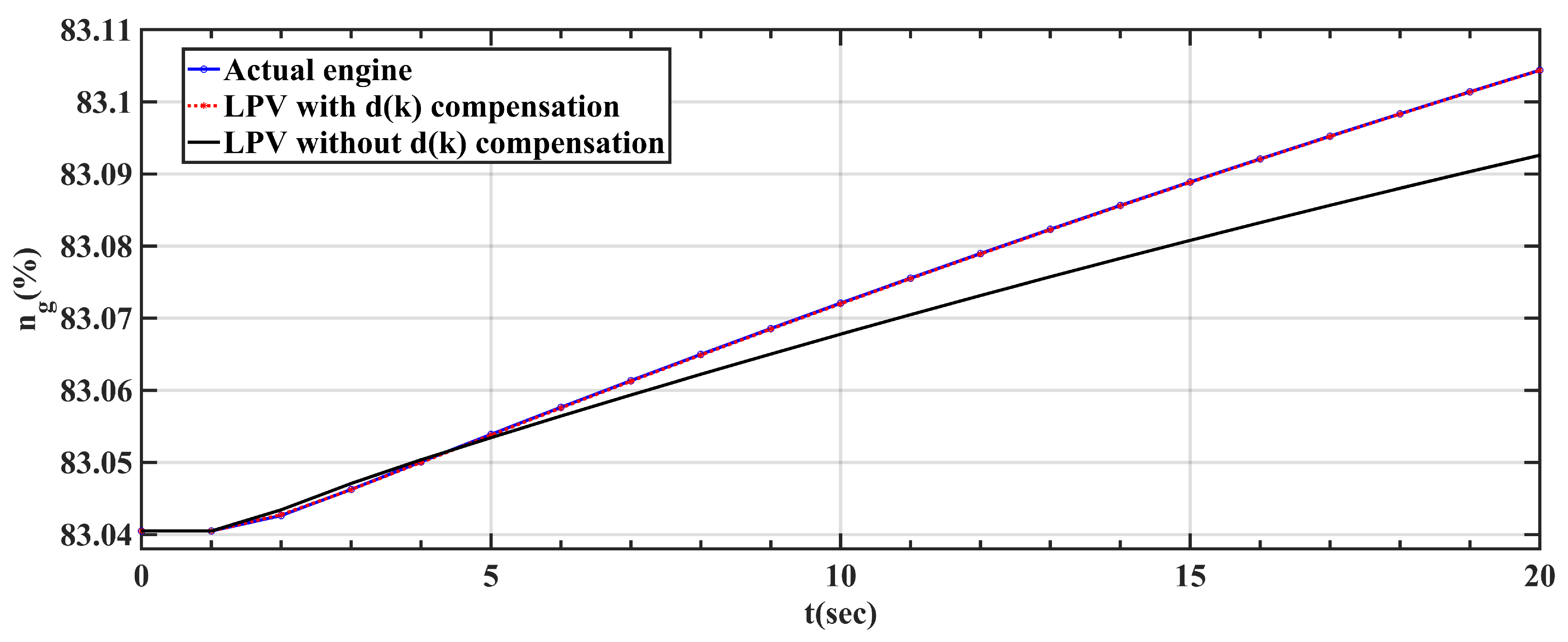
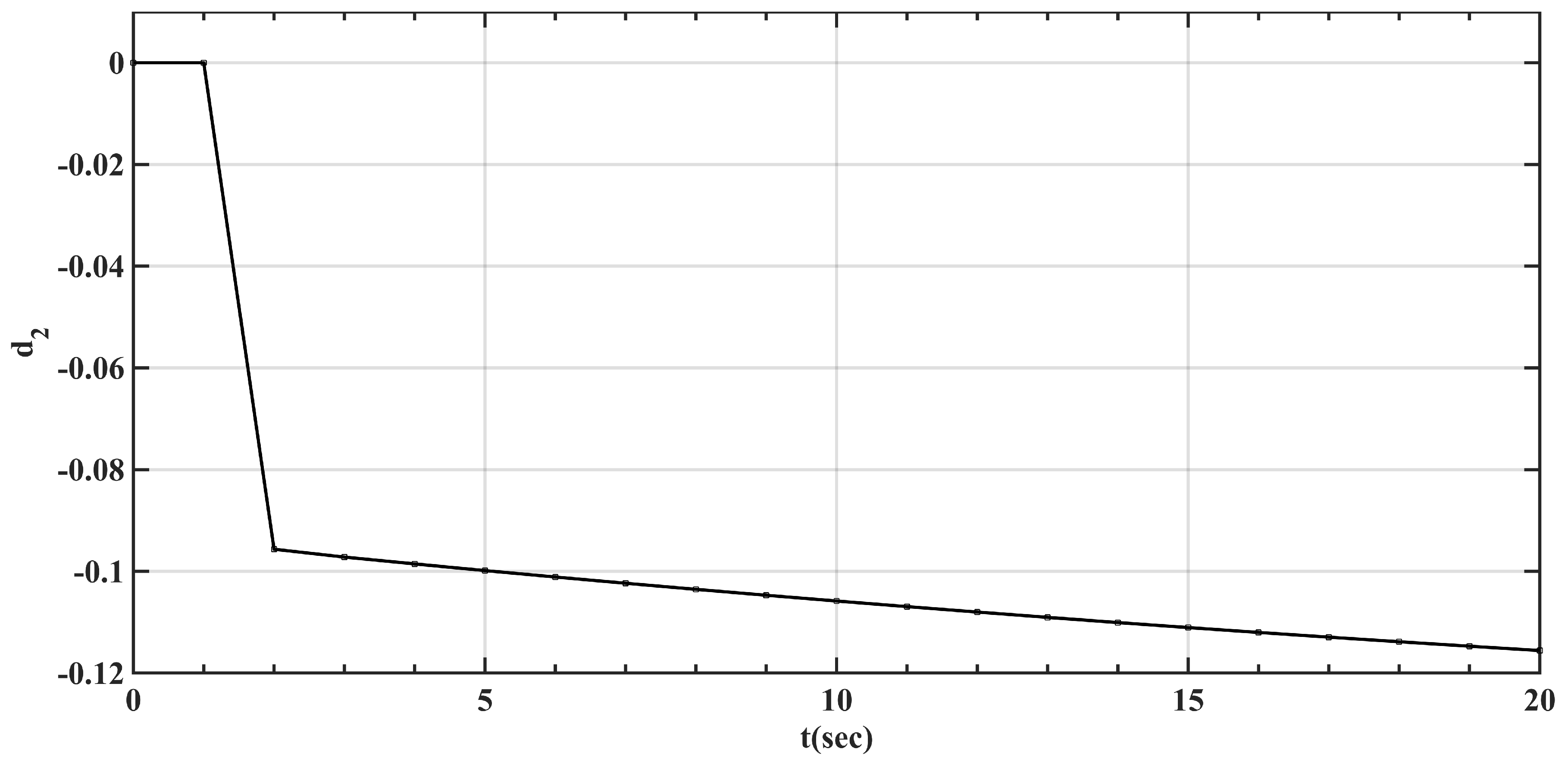
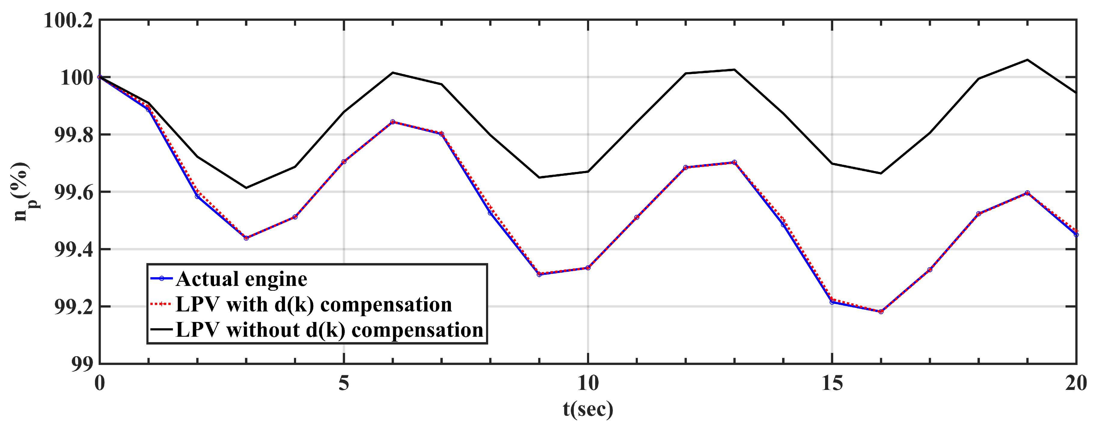
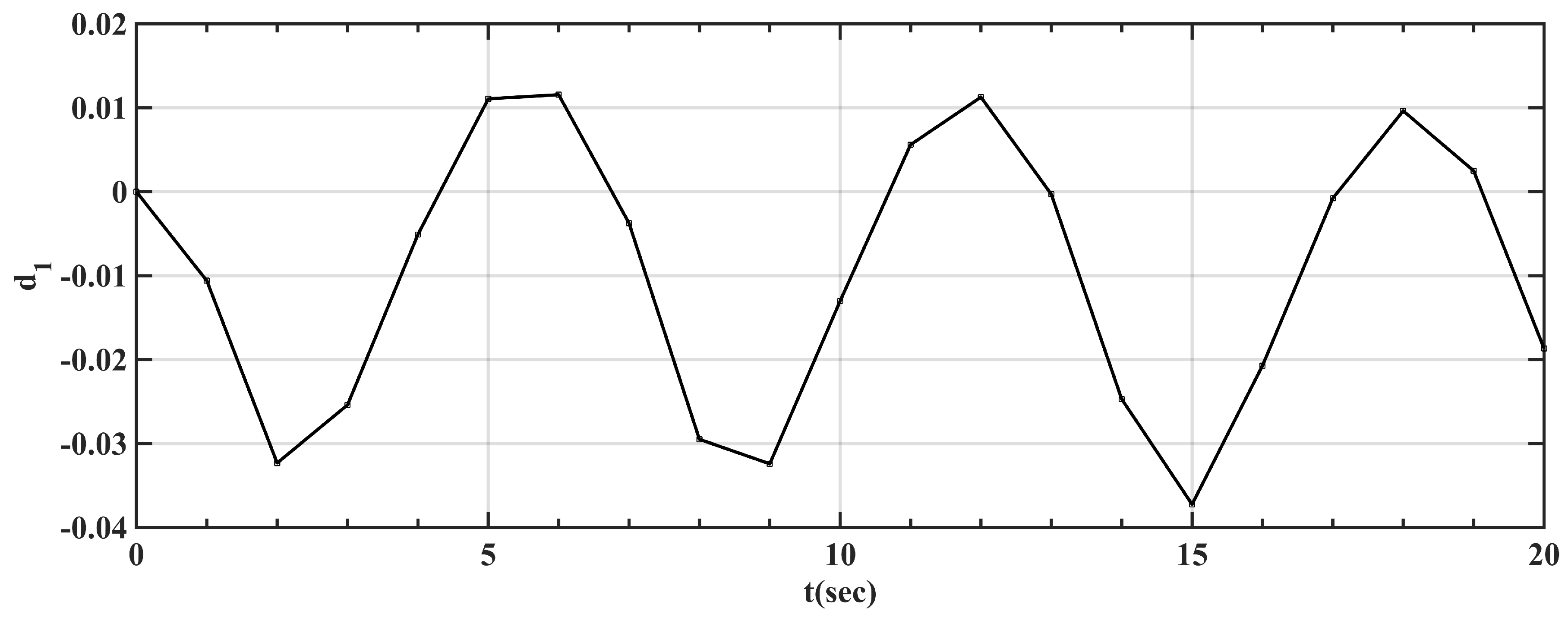
3.3. Validation of D-ESO

Now D-ESO has been developed above, we illustrate the effectiveness of D-ESO by carrying out a set of simulations.

Consider the case of ${\mathrm{w}}_{\mathrm{f}}=0.0319(\mathrm{kg}/\mathrm{s})$ and xcpc being a step signal (10–30%, Figure 5) as the inputs of a turbo-shaft engine/rotor system. From Figure 6 and Figure 7 we can see that LPV model and nonlinear system can tally well after the compensation of the D-ESO. Figure 8 and Figure 9 are the disturbance values being observed.

In fact, even if we provide the turbo-shaft engine/rotor system with an unreasonable and hash input, D-ESO can still guarantee that the LPV model fits very well with the actual engine system. While for the case without compensation, LPV model will fail to do so. Let ${\mathrm{w}}_{\mathrm{f}}=0.0319(\mathrm{kg}/\mathrm{s})$ and xcpc be a sine signal as in Figure 10; the comparison results of states and disturbances are presented in Figure 11 to Figure 12, and Figure 13 to Figure 14, respectively. Therefore, D-ESO as designed in this paper can well eliminate errors between LPV systems and real engine systems and be used in practical control systems.

4. D-ESO-Based Constrained Full-State MPC Controller

As we have above an LPV model compensated by D-ESO that can simulate real engine behavior well, an MPC controller can now be built by using the compensated LPV model as a predictive model (see Figure 15).

4.1. Control Objective

The control objective of the turbo-shaft engine is to keep the power turbine rotating at a constant speed (e.g., ${\mathrm{n}}_{\mathrm{p}}=100$%), considering the maneuvering and dynamic characteristics of the helicopter.

In this paper, we select the gas turbine speed ${\mathrm{n}}_{\mathrm{g}}$ as the tracking signal to realize the control of ${\mathrm{n}}_{\mathrm{p}}$ indirectly. The causes are shown as follows.

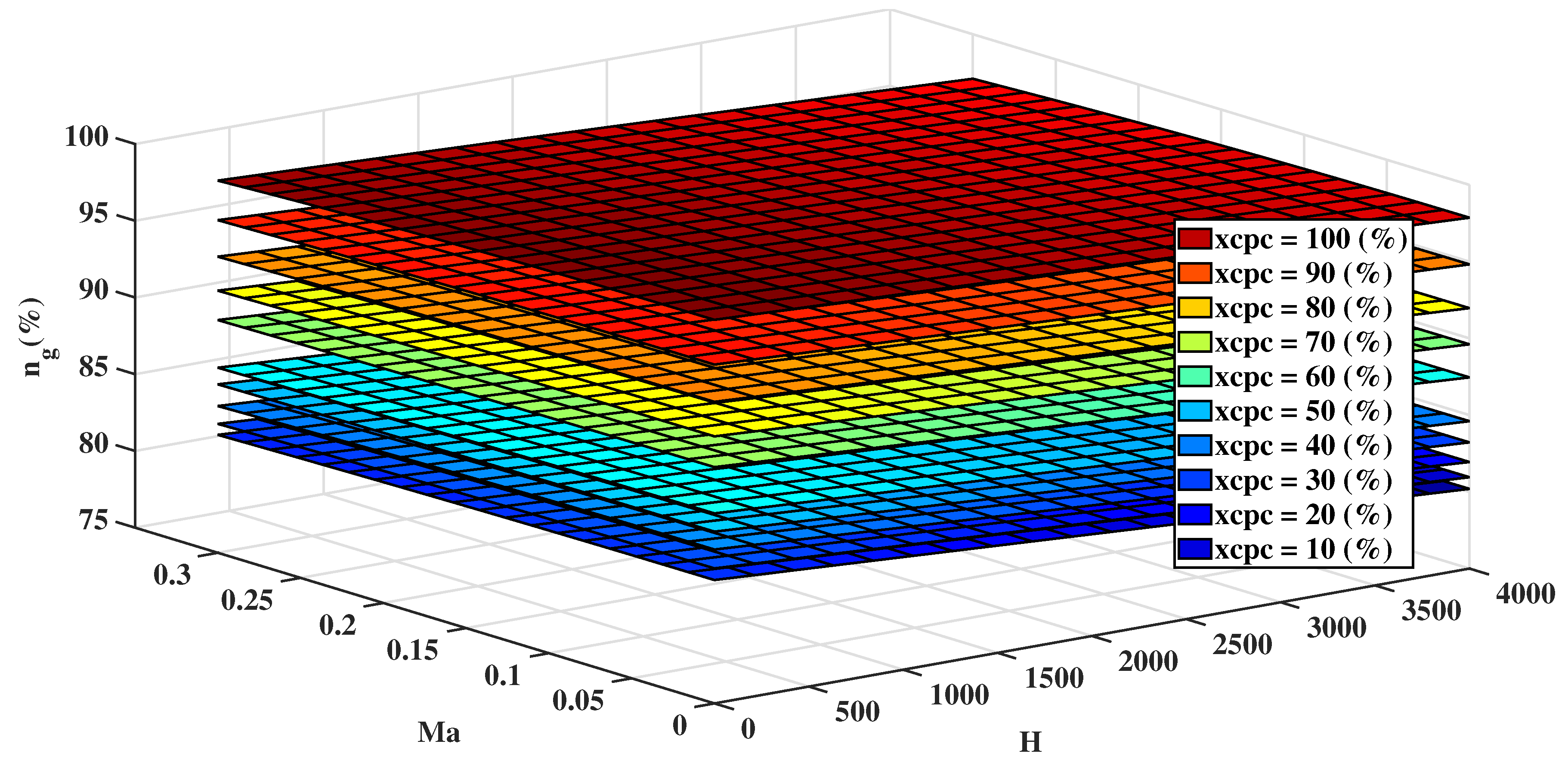
• Rationality. When the collective pitch input $\mathrm{xcpc}$ and flight conditions (operation altitude $\mathrm{H}$, Mach number $\mathrm{Ma}$) are all specified, there exists a one-to-one mapping relationship between ${\mathrm{n}}_{\mathrm{g}}$ and ${\mathrm{n}}_{\mathrm{p}}$.
• Feasibility. The relationship mentioned above can be realized by establishing the three-dimension model, see Figure 16.
• Superiority. The benefit is that the fast response of ${\mathrm{n}}_{\mathrm{g}}$ is fully utilized so that the control window of MPC is relatively smaller. In this way, the computational cost will be reduced.

4.2. MPC Controller Design

From this section, based on the D-ESO compensated LPV model constructed above, the design flow of MPC will be proposed.

(1) First, let $X={\left[\begin{array}{c}x\left(k\right),u\left(k-1\right)\end{array}\right]}^T$, $\Delta u\left(k\right)=u\left(k\right)-u\left(k-1\right)$ and $n_y$ be the output predictive horizon, the predictive equation of state variables can be then obtained,

$$\left[\begin{array}{c}x\left(k+1\right)\\ x\left(k+1\right)\\ ⋮\\ x\left(k+n_y\right)\end{array}\right]=P_{xx}X+H_x\left[\begin{array}{c}\Delta u\left(k\right)\\ \Delta u\left(k+1\right)\\ ⋮\\ \Delta u\left(k+n_y-1\right)\end{array}\right]+D_x+W_x.$$

(23)

Remark 2.

For the convenience of reading, the derivation process of (23) and the expressions of $D_x$, $W_x$, $P_{xx}$, $H_x$ can be seen in Appendix A (Equations (A1)–(A4)).

(2) Secondly, based on (1), the predictive equation of tracking signal can be described as:

$$\begin{array}{c}\hfill \left[\begin{array}{c}{y}_t\left(k+1\right)\\ y_t\left(k+2\right)\\ ⋮\\ y_t\left(k+n_y\right)\end{array}\right]=P_{t}X+H_t\left[\begin{array}{c}\Delta u\left(k\right)\\ \Delta u\left(k+1\right)\\ ⋮\\ \Delta u\left(k+n_y-1\right)\end{array}\right]+{\mathcal{D}}_t+{\mathcal{W}}_t.\end{array}$$

(24)

Remark 3.

For the convenience of reading, the derivation process of (24) and the expressions of ${\mathcal{D}}_t$, ${\mathcal{W}}_t$, $P_t$, $H_t$ can be seen in Appendix A (Equation (A5)).

(3) Thirdly, the predictive model of limit parameter $y_l$ can also be obtained,

$$\begin{array}{c}\hfill \left[\begin{array}{c}{y}_l\left(k+1\right)\\ y_l\left(k+2\right)\\ ⋮\\ y_l\left(k+n_y\right)\end{array}\right]=P_{l}X+H_l\left[\begin{array}{c}\Delta u\left(k\right)\\ \Delta u\left(k+1\right)\\ ⋮\\ \Delta u\left(k+n_y-1\right)\end{array}\right]+{\mathcal{D}}_l+{\mathcal{W}}_l.\end{array}$$

(25)

Remark 4.

For the convenience of reading, the derivation process of (25) and the expressions of ${\mathcal{D}}_l$, ${\mathcal{W}}_l$, $P_l$, $H_l$ can be seen in Appendix A (Equation (A6)).

(4) Considering the energy form of tracking error and incremental input, the objective function is described below.

$$J=\sum _{i=1}^{n_y}e{\left(k+i\right)}^{T}e\left(k+i\right)+\lambda \sum _{i=1}^{n_u-1}\Delta u{\left(k+i\right)}^T\Delta u\left(k+i\right)$$

(26)

where $n_u$ is control horizon, $\lambda >0$, $e\left(k+i\right)=r\left(k+i\left|k\right.\right)-y_t\left(k+i\left|k\right.\right)$.

(5) In this article, three constraint cases are considered: case one) $u_{min}\le u\left(k+i\right)\le u_{max}$; case two) $\Delta u_{min}\le \Delta u\left(k+i\right)\le \Delta u_{max}$; and case three) $y_{lmin}\le y_l\left(k+i\right)\le y_{lmax}$.

Constraints in three cases all need to be converted to the matrix forms represented by $\Delta u$. Note that for brevity, the detailed deducing is omitted here (see [5] for more information).

$$caseone:\left\{\begin{array}{c}{C}_m\Delta U\left(k\right)\le dumax\left(k\right)\\ -C_m\Delta U\left(k\right)\le dumin\left(k\right)\end{array}\right.$$

(27)

$$casetwo:\left\{\begin{array}{c}\Delta U\left(k\right)\le \Delta dumax\\ -\Delta U\left(k\right)\le -\Delta dumin\end{array}\right.$$

(28)

$$casethree:\left\{\begin{array}{c}{H}_l\Delta U\left(k\right)\le dymax\\ -H_l\Delta U\left(k\right)\le dymin\end{array}.\right.$$

(29)

Remark 5.

For the convenience of reading, the expressions of $C_m$, $dumax$, and $dumin$ in (27), $\Delta dumax$ and $\Delta dumin$ in (28), and $dymax$, $dymin$, and $H_l$ in (29) can be seen in Appendix B.

In conclusion, based on the D-ESO, MPC controller design of turbo-shaft engine can be converted to the following optimization problem,

$$\begin{array}{c}\underset{\Delta U}{min}J={\displaystyle \sum _{i=1}^{n_y}}e{\left(k+i\right)}^{T}e\left(k+i\right)+\lambda {\displaystyle \sum _{i=1}^{n_u-1}}\Delta u{\left(k+i\right)}^T\Delta u\left(k+i\right)\hfill \\ st.F\Delta U\left(k\right)\le {\rm Y}\left(k\right)\hfill \end{array}$$

(30)

where

$$F=\left[\begin{array}{cccccc}{C}_m& -C_m& I& -I& H_l& -H_l\end{array}\right]$$

$${\rm Y}\left(k\right)=\left[\begin{array}{cccccc}dumax\left(k\right)& dumin\left(k\right)& \Delta dumax& \Delta dumin& dymax\left(k\right)& dymin\left(k\right)\end{array}\right]$$

By letting $\Delta u\left(k\right)=u\left(k\right)-u\left(k-1\right)$, the advantages of increment control can be introduced in the controller.

Note that: since that the future disturbances are unknown, then in the above deducing process, we suppose that $\mathrm{d}\left(k+i\right)=\mathrm{d}\left(k\right)$ for $i=1,\cdots ,n_y-1$. Similarly, $w\left(k+i\right)=w\left(k\right)$ for $i=1,\cdots ,n_y$.

5. Simulation and Discussion

For verifying the validity of the method proposed in this paper, simulations are carried out and contrasted with the traditional M-M-STC controller (see Figure 17).

The logical structure diagram of the MPC controller for the integrated turbo-shaft engine/rotor system is provided as Figure 18. Based on this, we realize the control simulation of the integrated turbo-shaft engine/rotor model using the MATLAB/Simulink tool box. It should be noted that the simulations are all under standard atmosphere. During the whole process, the control goal is to keep the speed of power turbine constant and those limit parameters within assigned region by adjusting the fuel flow of MPC. For convenience, this paper regards compressor surge prevention as an example to verify the effectiveness of this controller.

The required system data of MPC can be seen in

Table 1. The state space system matrices around the equilibrium points.

Equilibrium Points	A	B	${\mathit{B}}_{\mathit{w}}$
$\mathrm{xcpc}=20$	$\left[\begin{array}{cc}0.9824& -4.4823\times {10}^{-4}\\ 4.7938\times {10}^{-4}& 0.9998\end{array}\right]$	$\left[\begin{array}{c}0.0077\\ 1.5442\times {10}^{-4}\end{array}\right]$	$\left[\begin{array}{c}1.4970\times {10}^{-8}\\ -6.6592\times {10}^{-5}\end{array}\right]$
$\mathrm{xcpc}=40$	$\left[\begin{array}{cc}0.9778& -4.1206\times {10}^{-4}\\ 6.8808\times {10}^{-4}& 0.9997\end{array}\right]$	$\left[\begin{array}{c}0.0070\\ 1.8595\times {10}^{-4}\end{array}\right]$	$\left[\begin{array}{c}3.1379\times {10}^{-8}\\ -1.5171\times {10}^{-4}\end{array}\right]$
$\mathrm{xcpc}=60$	$\left[\begin{array}{cc}0.9721& -3.7028\times {10}^{-4}\\ 6.7459\times {10}^{-4}& 0.9995\end{array}\right]$	$\left[\begin{array}{c}0.0067\\ 2.0649\times {10}^{-4}\end{array}\right]$	$\left[\begin{array}{c}6.4652\times {10}^{-8}\\ -3.4746\times {10}^{-4}\end{array}\right]$
$\mathrm{xcpc}=80$	$\left[\begin{array}{cc}0.9701& -2.9770\times {10}^{-4}\\ 0.0011& 0.9992\end{array}\right]$	$\left[\begin{array}{c}0.0062\\ 2.3112\times {10}^{-4}\end{array}\right]$	$\left[\begin{array}{c}7.2039\times {10}^{-8}\\ -4.8128\times {10}^{-4}\end{array}\right]$
$\mathrm{xcpc}=100$	$\left[\begin{array}{cc}0.9665& -3.1465\times {10}^{-4}\\ 9.0057\times {10}^{-4}& 0.9988\end{array}\right]$	$\left[\begin{array}{c}0.0061\\ 2.3171\times {10}^{-4}\end{array}\right]$	$\left[\begin{array}{c}1.0173\times {10}^{-7}\\ -6.4248\times {10}^{-4}\end{array}\right]$

and

Table 2. The state space system matrices around the equilibrium points.

Equilibrium Points	${\mathit{C}}_{\mathit{t}}$	${\mathit{D}}_{\mathit{t}}$	${\mathit{D}}_{\mathbf{wt}}$	${\mathit{C}}_{\mathit{l}}$	${\mathit{D}}_{\mathit{l}}$	${\mathit{D}}_{\mathbf{wl}}$
$\mathrm{xcpc}=20$	$\left[\begin{array}{cc}1& 0\end{array}\right]$	0	0	$\left[\begin{array}{cc}-1.3863& 1.3993\times {10}^{-4}\end{array}\right]$	$1.1882$	0
$\mathrm{xcpc}=40$	$\left[\begin{array}{cc}1& 0\end{array}\right]$	0	0	$\left[\begin{array}{cc}-1.6635& 1.0997\times {10}^{-4}\end{array}\right]$	$1.0208$	0
$\mathrm{xcpc}=60$	$\left[\begin{array}{cc}1& 0\end{array}\right]$	0	0	$\left[\begin{array}{cc}-1.5116& 5.2836\times {10}^{-5}\end{array}\right]$	$0.7997$	0
$\mathrm{xcpc}=80$	$\left[\begin{array}{cc}1& 0\end{array}\right]$	0	0	$\left[\begin{array}{cc}-1.6287& 3.6062\times {10}^{-5}\end{array}\right]$	$0.6313$	0
$\mathrm{xcpc}=100$	$\left[\begin{array}{cc}1& 0\end{array}\right]$	0	0	$\left[\begin{array}{cc}-0.7750& 5.7269\times {10}^{-5}\end{array}\right]$	$0.5153$	0

; limited by space we do not write everything in detail.

MPC Controller Validation

Simulation begins at 0 s and ends at 350 s. Under the standard atmosphere ($\mathrm{H}=0$, $\mathrm{Ma}=0$), the collective pitch $\mathrm{xcpc}$ raises up to a full-load state in a stepwise manner in the first half time, and then reduces to a 10% position in the second half of the simulation time (Figure 19).

MPC controller parameters are designed as in

Table 3. Parameter settings of MPC at the standard atmospheric state.

Parameters	${\mathit{n}}_{\mathit{y}}$	${\mathit{n}}_{\mathit{u}}$	$\mathit{\lambda }$
$\mathrm{Value}$	7	3	$0.5$

. Meanwhile, the parameter constraints during the control process of the transient state are given in

Table 4. Constraint parameter settings.

Parameters	${\mathit{u}}_{\mathbf{max}}$	${\mathit{u}}_{\mathbf{min}}$	$\mathbf{\Delta }{\mathit{u}}_{\mathbf{max}}$	$\mathbf{\Delta }{\mathit{u}}_{\mathbf{min}}$	$\mathbf{S}{\mathbf{M}}_{\mathbf{min}}$
$\mathrm{Value}$	0.1043 (kg/s)	0.031 (kg/s)	0.003	$-0.003$	$2(\%)$

.

Figure 20 is the input fuel flow curves under two different control strategies (M-M-STC and MPC); Figure 21 reflects the fuel flow rate; The surge margin curves of the compressor are presented in Figure 22; the last two figures (Figure 23 and Figure 24) correspond to the speed of the gas turbine and power turbine respectively.

From Figure 20, it can be seen that MPC is competent for handling the constraints: During the whole process (loading or unloading process), the input of ${\mathrm{w}}_{\mathrm{f}}$ remains between $u_{max}$ and $u_{min}$ without exceeding the input limit described in Table 4. Figure 21 further proves the validity of MPC in dealing with the constraints of the input rate $\Delta {\mathrm{w}}_{\mathrm{f}}$. From Figure 22, the line of surge margin $\mathrm{SM}$ is controlled within the limit range (given in Table 4) under MPC strategy. Therefore, it can be confirmed that MPC can be well applied to control problems with constraints. This ability originates from the fact that only sequences expected to fulfill the constraints can be taken into consideration as control candidates. This can be shown by Equation (30). MPC is an optimization problem with inputs subjected to certain constraints. Those input constraints ensure that a certain system output or input parameters will not exceed assigned constraints. It is possible and easy to construct constraints which capture the limitation on input, output, state magnitudes, and rates.

In addition to constraint handling, transient performance can be guaranteed on MPC`s anticipatory character as a performance function. From Figure 23 and Figure 24, we can see the MPC proposed here can also provide the engine with good steady-state performance and fast transient behavior in response to the step change of propeller power load. In contrast to the traditional M-M-STC method, the drop of ${\mathrm{n}}_{\mathrm{p}}$ under MPC control declines to 1.9%, and its overshoot is reduced to 1.87%. Furthermore, as shown in Figure 24, during the whole optimization process, the MPC is capable of shortening the transient process of ${\mathrm{n}}_{\mathrm{p}}$ significantly. Hence, the conservativeness of the M-M-STC method can also be overcome.

Above all, MPC can not only perform well during the steady-state and transient operation, but also can be applied to control problems with constraints similar to the M-M-STC method. Meanwhile, MPC removes the complex Min-Max selection logic so that it has a simpler design structure than M-M-STC. From this point, MPC is superior to M-M-STC. Furthermore, unlike M-M-STC, MPC’s design process is also simple and easy to handle. In practical engineering, in order to obtain high precise accelerating (ACC-line in Figure 25) and decelerating (DEC-line in Figure 25) fuel plans with M-M-STC, this requires repeat tests and modifying process which will lead to a larger cost of time and manpower. Otherwise, M-M-STC cannot always guarantee that the limiting parameters are kept within the specified range without being well tested. In this respect, we can find the proof from the local sub-graphs of Figure 20, Figure 25, and Figure 22.

On the whole, the MPC controller can realize the tracking problem of a turbo-shaft engine/rotor system. Meanwhile, it can keep the limit parameters in the specified range at the same time. Moreover, MPC overcomes the drawbacks (e.g., conservative property, difficulty to obtain, and complex structure) of the M-M-STC method.

6. Conclusions

The research work of this paper includes the following two parts: (1) In order to compensate for the mismatch of the predictive model, the D-ESO has been proposed in this paper; moreover, the convergence conditions are given in Theory 1; (2) Using the LPV model corrected by D-ESO, we develop a predictive controller to realize the constrained full-state control. Several specific conclusions have been drawn as follows:

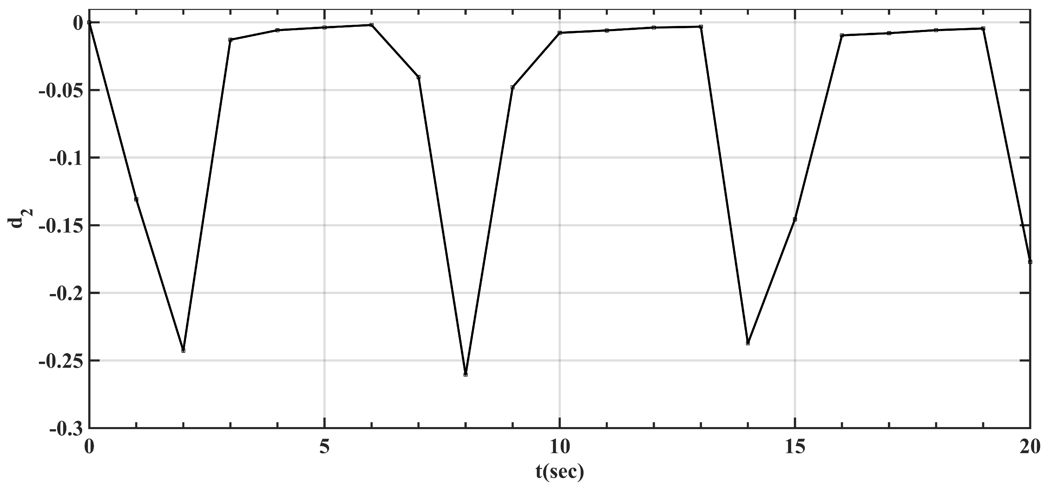
• Through the above simulation, the effectiveness of D-ESO has been proven as follows: D-ESO can compensate the linearization error between LPV and real turbo-shaft engine/rotor systems.
• Convergence conditions of D-ESO are deduced in Theory 1.
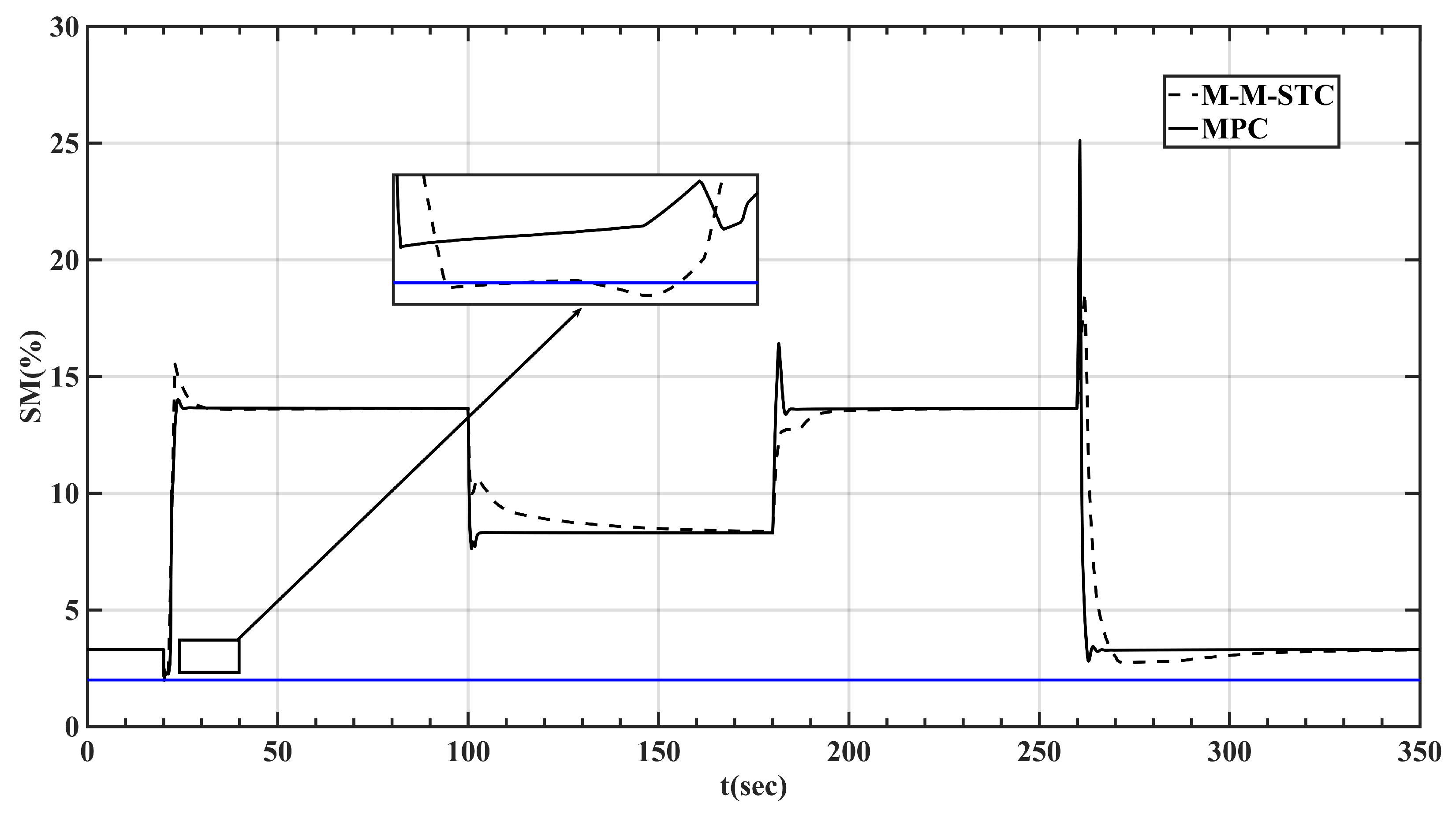
• During the transient state process, MPC can keep the limit parameters within the limited range. Meanwhile, it leaves out the Min-Max selection logic, which makes the controller structure more concise and simpler.
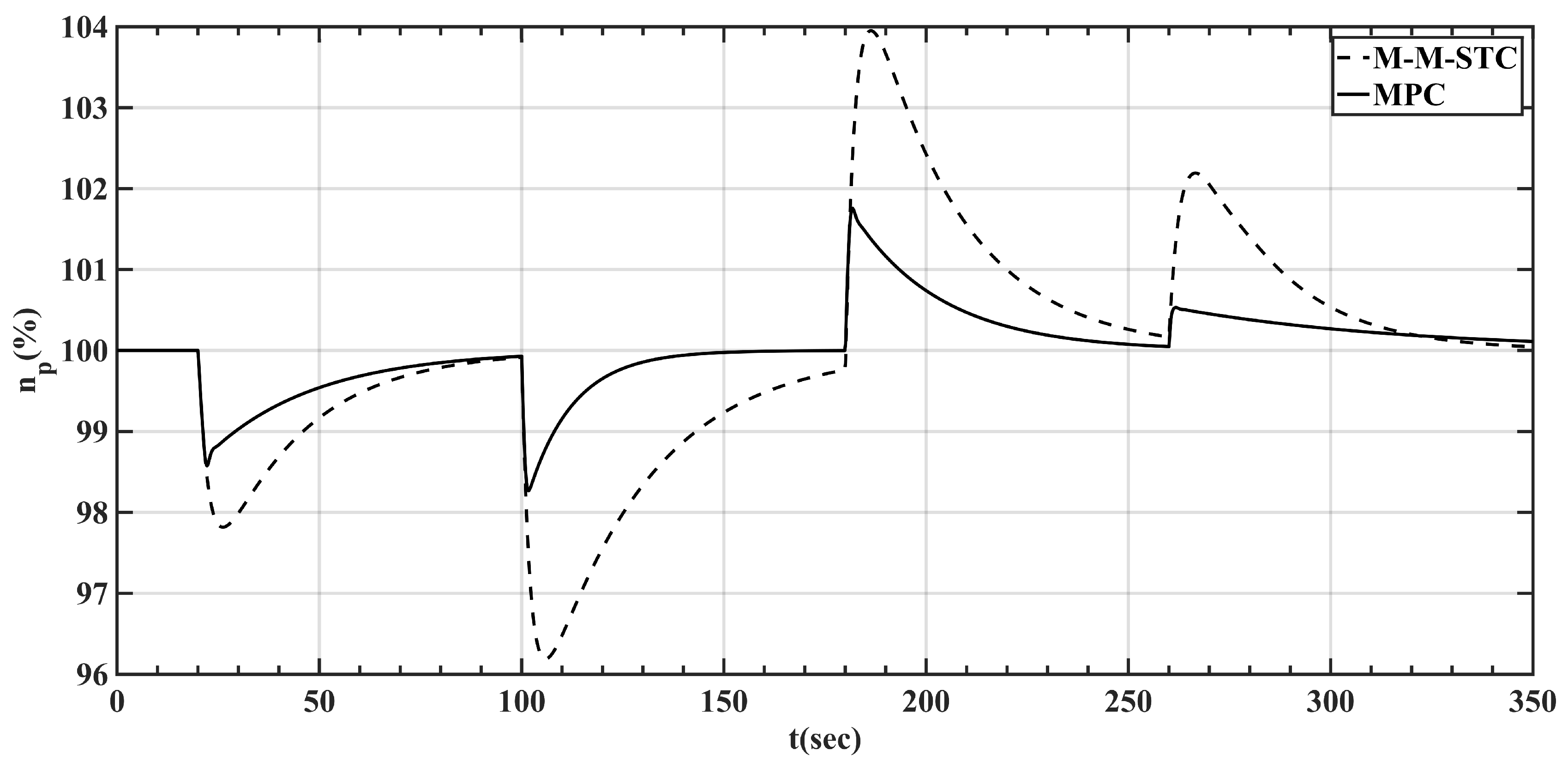
• Fast response and high-quality control of a turbo-shaft engine can be available. The drop of the power turbine speed is less than 2%. In addition, the steady-state error is below 0.2% through adopting the MPC controller based on the LPV model and D-ESO.

References

1. Liu, X.F.; Luo, C.S. Stability analysis for GE T700 turboshaft distributed engine control systems. IEEE Access 2017, 5, 22485–22491. [Google Scholar] [CrossRef]
2. Pakmehr, M.; Fitzgerald, N.; Eric, F. Physics based dynamic modeling of a turboshaft engine driving a variable pitch propeller. J. Propuls. Power 2016, 32, 646–658. [Google Scholar] [CrossRef]
3. Zhang, C.Y.; Gummer, V. The potential of helicopter turboshaft engines incorporating highly effective recuperators under various flight conditions. Aerosp. Sci. Technol. 2019, 88, 84–94. [Google Scholar] [CrossRef]
4. Andrea, G.; Ernesto, B. Preliminary study on a wide-speed-range helicopter rotor/turboshaft system. J. Aircr. 2012, 49, 1032–1038. [Google Scholar]
5. Smith, B.J.; Zagranski, R.D. Next generation control system for helicopter engines. In Proceedings of the International Annual Forum of AHS, Washington, DC, USA, 9–11 May 2001. [Google Scholar]
6. Smith, B.J.; Zagranski, R.D. Closed loop bench testing of the next generation control system for helicopter engines. In Proceedings of the International Annual Forum of AHS, Montreal, QC, Canada, 11–13 June 2002. [Google Scholar]
7. Jaw, L.C.; Garg, S. Propulsion Control Technology Development in the United States: A Historical Perspective; Technical Report; The NASA STI Program Office: Washington, DC, USA, 2005. [Google Scholar]
8. Merrill, W.; Lehtinen, B.; Zeller, J. The role of modern control theory in the design of controls for aircraft turbine engines. J. Guid. Control Dyn. 1984, 7, 652–661. [Google Scholar] [CrossRef]
9. Dang, W.; Wang, X.; Wang, H.W. Design of transient state control mode based on rotor acceleration. In Proceedings of the International Bhurban Conference on Applied Sciences and Technology, Islamabad, Pakistan, 13–17 January 2015. [Google Scholar]
10. Richter, H. Advanced Control of Turbofan Engines; Springer: Berlin, Germany, 2011. [Google Scholar]
11. Richter, H. A multi-regulator sliding mode control strategy for output-constrained systems. Automatica 2011, 47, 2251–2259. [Google Scholar] [CrossRef]
12. Krstic, M.; Banaszuk, A. Multivariable adaptive control of instabilities arising in jet engines. Control Eng. Pract. 2006, 14, 833–842. [Google Scholar] [CrossRef]
13. Brunell, B.J.; Viassolo, D.E.; Prasanth, R. Model adaptation and nonlinear model predictive control of an aircraft engine. In Proceedings of the ASME Turbo Expo, Vienna, Austria, 14–17 June 2004. [Google Scholar]
14. Richter, H.; Singaraju, A.; Lit, J.S. Multiplexed predictive control of a large commercial turbofan engine. J. Guid. Control Dyn. 2008, 31, 273–281. [Google Scholar] [CrossRef]
15. Cutler, C.R.; Ramaker, B.L. Dynamic matrix control—A computer control algorithm. In Proceedings of the Joint Automatic Control Conference, San Francisco, CA, USA, 13–15 August 1980. [Google Scholar]
16. Clarke, D.W.; Mohtadi, C.; Tuffs, P.S. Generalized predictive control-part I: the basic algorithm. Automatica 1987, 23, 137–148. [Google Scholar] [CrossRef]
17. Morteza, M.G.; Ali, R. Comparison of model predictive controller and Min-Max approach for aircraft engine fuel control. In Proceedings of the International Conference on Control, Instrumentation, and Automation, Shiraz, Iran, 21–23 November 2017. [Google Scholar]
18. Garriga, J.L.; Soroush, M. Model predictive control tuning methods: A review. Ind. Eng. Chem. Res. 2010, 49, 3505–3515. [Google Scholar] [CrossRef]
19. Chen, W.H.; Ballance, D.J.; Reilly, O.J. Model predictive control of nonlinear systems: Computational burden and stability. Syst. Control Lett. 2000, 147, 387–394. [Google Scholar] [CrossRef]
20. Morari, M.; Lee, J.H. Model predictive control: Past, present and future. Comput. Chem. Eng. 1999, 23, 667–682. [Google Scholar] [CrossRef]
21. Wan, Z.Y.; Kothare, M.V. Robust output feedback model predictive control using off-line linear matrix inequalities. J. Process. Control 2002, 12, 763–774. [Google Scholar] [CrossRef]
22. DeCastro, J.A. Rate-based model predictive control of turbofan engine clearance. J. Propuls. Power 2007, 23, 804–813. [Google Scholar] [CrossRef]
23. Su, Y.X.; Duan, B.Y. Disturbance-rejection high-precision motion control of a Stewart platform. IEEE Trans. Control Syst. Technol. 2004, 12, 364–374. [Google Scholar] [CrossRef]
24. Zheng, Q.; Dong, L.l.; Lee, D.H.; Gao, Z.Q. Active disturbance rejection control and implementation for MEMS gyroscopes. IEEE Trans. Control Syst. Technol. 2009, 17, 1432–1438. [Google Scholar] [CrossRef]
25. Zheng, Q.; Chen, Z.z.; Gao, Z.Q. A dynamic decoupling control approach and its applications to chemical processes. In Proceedings of the American Control Conference, New York, NY, USA, 9–13 July 2007; pp. 5176–5181. [Google Scholar]
26. Li, Z.l.; Xu, F.; Liang, D.N.; Chen, H. Design of model predictive controller based on extended state observer. In Proceedings of the Chinese Control and Decision Conference, Chongqing, China, 28–30 May 2017; pp. 7421–7426. [Google Scholar]
27. Zhao, Z.L.; Guo, B.Z. On convergence of nonlinear active disturbance rejection control for SISO nonlinear systems. J. Dyn. Control Syst. 2016, 22, 385–413. [Google Scholar] [CrossRef]
28. Praly, L.; Jiang, Z.P. Linear output feedback with dynamic high gain for nonlinear systems. Syst. Control Lett. 2004, 53, 107–116. [Google Scholar] [CrossRef]
Figure 1. Structure of turbo-shaft engine.
Energies 12 04496 g001
Figure 2. Component level model of turbo-shaft engine/rotor system.
Energies 12 04496 g002
Figure 3. Predictive model compensated by Disturbance based extended state observer (D-ESO).
Energies 12 04496 g003
Figure 4. The structure of D-ESO.
Energies 12 04496 g004
Figure 5. The input of collective pitch xcpc .
Energies 12 04496 g005
Figure 6. The response curves of n g .
Energies 12 04496 g006
Figure 7. The response curves of n p .
Energies 12 04496 g007
Figure 8. The disturbance term d 1 ( k ) .
Energies 12 04496 g008
Figure 9. The disturbance term d 2 ( k ) .
Energies 12 04496 g009
Figure 10. The input of collective pitch xcpc.
Energies 12 04496 g010
Figure 11. The response curves of n g .
Energies 12 04496 g011
Figure 12. The response curves of n p .
Energies 12 04496 g012
Figure 13. The disturbance term d 1 ( k ) .
Energies 12 04496 g013
Figure 14. The disturbance term d 2 ( k ) .
Energies 12 04496 g014
Figure 15. Model predictive control (MPC) controller with D-ESO.
Energies 12 04496 g015
Figure 16. The management plan of n g for the turbo-shaft engine/rotor system.
Energies 12 04496 g016
Figure 17. Min-Max structure and schedule-based transient controller (M-M-STC) structure.
Energies 12 04496 g017
Figure 18. Schematic diagram of MPC controller for turbo-shaft engine/rotor system.
Energies 12 04496 g018
Figure 19. The input of collective pitch xcpc .
Energies 12 04496 g019
Figure 20. The response curves of main fuel flow w f .
Energies 12 04496 g020
Figure 21. The response curves of the rate of main fuel flow Δ w f .
Energies 12 04496 g021
Figure 22. The response curves of surge margin SM .
Energies 12 04496 g022
Figure 23. The response curves of n g .
Energies 12 04496 g023
Figure 24. The response curves of n p .
Energies 12 04496 g024
Figure 25. The fuel supplying plan under M-M-STC (ACC- acceleration control plan; DEC- deceleration control plan).
Energies 12 04496 g025