Field Weakening Operation Control Strategies of PMSM Based on Feedback Linearization

Abstract

Based on current research into the mathematical model of the permanent magnet synchronous motor (PMSM) and the feedback linearization theory, a control strategy established upon feedback linearization is proposed. The Lie differential operation is performed on the output variable to obtain the state feedback of the nonlinear system, and the dynamic characteristics of the original system are transformed into linear dynamic characteristics. A current controller based on the input–output feedback linearization algorithm is designed to realize the input–output linearization control of the PMSM. The current controller decouples the d–q axis current from the flux linkage information of the motor and outputs a control voltage. When the motor speed reaches above the base speed, the field-forward and straight-axis current components are newly distributed to achieve field weakening control, which can realize the smooth transition between the constant torque region and weak magnetic region. Simulation and experimental results show the feasibility and viability of the strategy.

1. Introduction

Permanent magnet synchronous motor (PMSM) have been widely used in a variety of industrial applications due to their high power density, high efficiency, high reliability and wide constant power operating range [1]. In the running process of the motor, when the speed increases to the base speed, the stator terminal voltage reaches the inverter output limit value, the current regulator reaches saturation state, and the motor speed cannot continue to rise. In order to make the motor reach a higher speed, it is necessary to adopt corresponding measures to make the current regulator desaturated, regain the control ability of the current, and realize the rebalancing relationship between the motor speed and the back electromotive force. The flux weakening (FW) control strategy of PMSM first appeared in the 1980s [2]. It is pointed out that the stator current of the motor is constrained by the voltage limit circle and the current limit circle, and the maximum torque current curve is obtained. Through the study of vector control theory, there are two main ways to improve the weak magnetic performance: one is to optimize the structure of the motor body; the other is to study the flux weakening control from the control algorithm strategy [3]. This paper mainly researches on the flux weakening control algorithm, so the optimization of the weak magnetic field of the motor body structure is not described in detail.

The PMSM rotor structure is special and the flux linkage is constant, which makes the flux weakening control more complicated [4]. When the PMSM is running in the field weakening control zone, once the given torque is suddenly changed, the output voltage of the current controller is easy to saturate. At this time, the output torque performance of the motor will be affected, and in severe cases, the entire system will be out of control [5,6,7]. The six-step voltage method is a representative control approach that can improve the use of direct current (DC) bus voltage [8]. The single current regulator, including the voltage angle, has the voltage vector angle by proportional-integral (PI) adjustment of the d-axis current error and the speed expansion effect is good [9]. The feed forward flux weakening control strategy estimates the d-axis current using the motor parameters and the voltage limit circle, and the dynamic performance is good. However, when the motor parameters change, the control strategy is difficult to follow the optimal trajectory. Therefore, it is not common in practical applications, and is mostly used in the simulation process where the motor parameters are known and will not change [10,11,12]. The online parameter prediction control method estimates the d–q axis inductance, which reduces the dependence on the motor parameters. However, the derivation and calculation are cumbersome and complicated and are not highly recommended for various applications [13]. The control strategy of the d-axis current compensation is ideal for dynamic performance but requires precise parameters of the motor [14]. The gradient descent method weak field control can update the given value of the stator current according to the position of the weak magnetic region. The control method can adjust the weak magnetic running direction in real time, realize nonlinear control of the weak magnetic region, high control precision and fast response speed [15,16,17]. However, this algorithm is extremely complicated and has a large dependence on motor parameters. Professor Xu Longya of the Ohio State University proposed a single-current flux weakening control algorithm for various problems in the above flux weakening control method. In this control strategy, the d-axis reference voltage is still given by the d-axis current regulator output. However, the q-axis reference voltage is given externally, so that once the d-axis given current is determined, the q-axis given current can be directly obtained. This method relieves the shackles on the current regulator and broadens the range of weak magnetic acceleration [18]. Whereas, the control strategy itself has the disadvantages of poor load capacity and low power utilization, and can only operate in an electric state and cannot operate in a power generation state. Direct-flux vector control (DFVC) is derived from the direct torque control (DTC) idea. DTC is adopted when the motor runs below the base speed, which requires parameter calculation based on the motor model. When the motor enters the field weakening zone, the parameter calculation can be omitted. DFVC uses the current constraint condition when the motor runs in the maximum torque per voltage (MTPV) to determine whether flux weakening control is performed. The influence of constant power speed ratio (CPSR) on the weak magnetic property of the motor is fully considered [19,20,21,22].

This paper investigates the PMSM, and from the analysis of its topology and principles, a control strategy based on feedback linearization is proposed. Since the PMSM is a complex nonlinear system, favorable control performance can be obtained by decoupling the coupling term in its mathematical equation. The commonly used PI control decoupling is difficult to meet the performance requirements in the full speed range. Therefore, the feedback linearization theory is applied. The Lie differential operation of the output variable is used to obtain the required coordinate transformation and nonlinear system state feedback. The input–output feedback linearization of the PMSM is realized, and the feedback linearization algorithm is designed. The controller implements the decoupling control of the system. When the motor speed reaches the turning speed, the stator current vector and the cross-axis current vector have a certain angle, that is, the current lead angle. The stator current is re-allocated by controlling the current lead angle to control the current components of the cross-axis and the straight-axis. As the lead angle of the current increases, the direct current increases inversely, the cross-axis current decreases, and the motor changes smoothly to the flux weakening control zone. The simulation and experimental research into the control system demonstrate that the proposed control strategy is robust, and exhibits both stable and accurate dynamic tracking.

The organization of this paper is as follows: Section 2 analyzes the mathematical model of PMSM. Section 3 introduces the concept of flux weakening control. Section 4 designs the field weakening control strategy, and Section 5 provides the simulation results. Section 6 provides the experimental results. Section 7 summarizes this article.

2. PMSM Mathematical Model

To facilitate the analysis and application, the interference of the core parameters, such as core saturation, higher harmonics and eddy current on the motor parameters is temporarily disregarded. The voltage equation of PMSM in a synchronous rotating coordinate system is shown [23].

$$u_d=R_s{i}_d+\frac{d}{dt}{\psi }_d-{\omega }_e{\psi }_q.$$

(1)

$$u_q=R_s{i}_q+\frac{d}{dt}{\psi }_q+{\omega }_e{\psi }_d.$$

(2)

The flux linkage equation:

$${\psi }_d=L_d{i}_d+{\psi }_f.$$

(3)

$${\psi }_{\mathrm{q}}=L_{\mathrm{q}}{i}_q.$$

(4)

The electromagnetic torque is:

$$T_{em}=1.5p_n({\psi }_d{i}_q-{\psi }_q{i}_d).$$

(5)

Based on the theory of magnetic field orientation, the state equation of PMSM in a synchronous rotating coordinate system is:

$$\left[\begin{array}{l}{\dot{i}}_d\\ {\dot{i}}_q\\ {\dot{\omega }}_e\end{array}\right]=\left[\begin{array}{ccc}-R_s/L& n_p{\omega }_e& 0\\ n_p{\omega }_e& -R_s/L& -n_p{\psi }_f/L\\ 0& 1.5n_p{\psi }_f/J& -B/J\end{array}\right]\left[\begin{array}{c}{i}_d\\ i_q\\ {\omega }_e\end{array}\right]+\left[\begin{array}{c}{u}_d/L_d\\ u_q/L_q\\ -T_L/J\end{array}\right].$$

(6)

It can be seen from Equation (6) that the PMSM is a multi-variable system. There is a strong nonlinear coupling relationship between i_d, i_q and ω_e, which cannot be adjusted separately. Therefore, i_d and i_q need to be used in order to achieve decoupling.

The equation of mechanical motion:

$$T_{em}-T_L=J\frac{d{\omega }_m}{dt}+B{\omega }_m.$$

(7)

When the motor is in stable operation, the integral amount can be ignored and the voltage equation can be simplified as:

$$u_d=R_s{i}_d-{\omega }_e{L}_{\mathrm{q}}{i}_q.$$

(8)

$$u_q=R_s{i}_d+{\omega }_e{L}_d{i}_d+{\omega }_e{\psi }_f.$$

(9)

When the motor is running at a high speed, the voltage equation can be simplified as:

$$u_d=-{\omega }_e{L}_q{i}_q.$$

(10)

$$u_q={\omega }_e{L}_d{i}_d+{\omega }_e{\psi }_f.$$

(11)

Substituting Equations (3) and (4) into Equation (5) yields:

$$T_{\mathrm{e}m}=1.5p_n[{\psi }_f{i}_q+(L_d-L_q)i_d{i}_q].$$

(12)

u_d, u_q, ψ_d and ψ_q are the stator voltage and flux linkage components in the d–q coordinate system, respectively, where i_d and i_q are the direct axis and the intersecting axis current, respectively, while L_d and L_q are the direct axis and the intersecting axis inductance, respectively. Meanwhile, R_s is the stator resistance; ψ_f is the rotor flux; T_em is the electromagnetic torque output by the motor; T_L is the load torque; P_n is the motor pole pair; J is the moment of inertia; ω_e is the rotor angular velocity and ω_m is the mechanical angular velocity.

In Equation (12), the electromagnetic torque T_em consists of two parts such as reluctance torque and excitation torque. Since the L_d of the PMSM is usually smaller than L_q, the optimal control of the PMSM can be achieved by changing the reluctance torque.

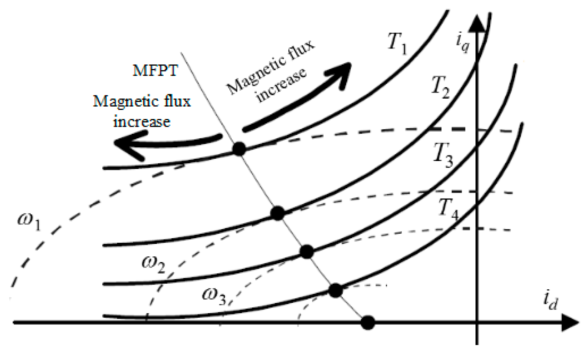
3. Field Weakening Operation Control

Assuming that the motor is in a steady state and ignoring its winding voltage drop, the motor d–q axis flux linkage equation is as follows [24,25,26]:

$$\{\begin{array}{l}{\psi }_q=L_q{i}_q=\rho L_d{i}_q\hfill \\ {\psi }_d=L_d{i}_d+{\varphi }_f\hfill \end{array}.$$

(13)

By combining Equation (13) with the motor torque Equation (5), the motor d–q axis composite flux linkage can be regarded as a function of the d-axis current. The functional equation is:

$${({\psi }_{dq})}^2={(\rho L_d{i}_q)}^2+{({\psi }_f+L_d{i}_d)}^2=\frac{{(\rho L_d{T}_e)}^2}{{[{\psi }_f-(\rho -1)L_d{i}_d]}^2}+({\psi }_f+L_d{i}_d).$$

(14)

From Equation (14), it can be found that the motor flux linkage increases as the d-axis current increases, and when the d-axis current reaches ${\psi }_f/(\rho -1)L_d$, the motor flux linkage reaches infinity.

$$\frac{d{({\psi }_{dq})}^2}{d{i}_d}=\frac{2{\rho }^2{L}_d{}^3{T}_e{}^2(\rho -1)}{{[{\psi }_f-(\rho -1)L_d{i}_d]}^3}+2L_d({\psi }_f+L_d{i}_d)=0.$$

(15)

When the running state of the motor satisfies the Equation (15), the flux linkage is a constant, and the voltage amplitude does not change under the condition that the rotational speed is constant. For the voltage limit ellipse, when the motor speed is fixed, the voltage amplitude of any working point on the ellipse is fixed, and the amplitude of the motor flux linkage is constant. The set of tangent points of the equal torque curve and the voltage limit ellipse is called the minimum flux per torque (MFPT) trajectory. On the equal torque curve, the variation of the flux amplitude is shown in Figure 1.

Figure 2 shows the curve of the operating point when the motor was weakly magnetically operated. The boundary line consisting of the maximum torque per ampere (MTPA) trajectory, the MFPT trajectory and the current limit circular trajectory divides the operating range of the motor into three parts.

In the interval I, for a given torque command, the MTPA control algorithm is selected without considering the weak magnetic requirement, so the operating point of the motor in the interval I exists only on the MTPA trajectory. In interval II, the motor needs to output a larger current for a given torque command, but it is close to the MFPT track, the required flux linkage amplitude becomes smaller. In the interval III, for a given torque command, the current and flux linkage of the motor are the largest, so the actual control should ensure that the motor operating point does not enter the interval III.

When the motor needs weak field in the operation of the interval II, its working point should be moved to the MFPT from the MTPA along the equal torque curve. At this time, the motor flux linkage is minimized, and the motor operating point will not continue to move along the equal torque curve. However, as the rotational speed continues to rise, the MFPT trajectory gradually moves toward the C point.

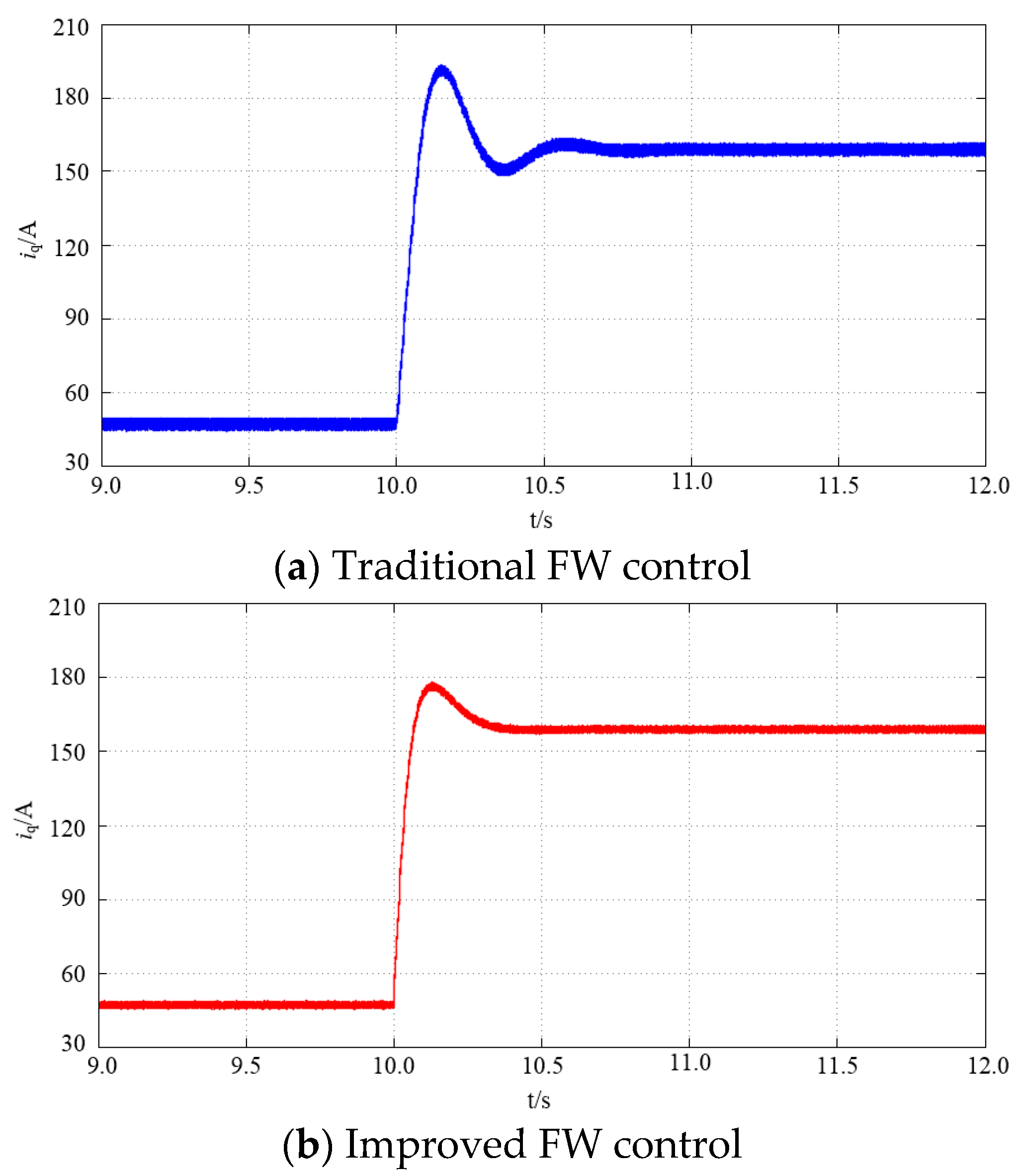
4. The Improved Flux Weakening Control Strategy

When the motor speed reaches the rated speed, the current regulator reaches saturation state, and the PMSM stator voltage and current reach the voltage limit circle and current limit circle of the inverter output. At this time, in order to further increase the motor speed, PMSM flux weakening control can be realized by increasing the direct shaft demagnetization current. The field weakening control usually has feedforward control and feedback control. The feedforward control is highly dependent on the motor parameters, and the speed regulation performance is poor, which is not commonly used in actual working conditions. Feedback control can be divided into negative straight axis current compensation method and current lead angle weak field control.

When the PMSM reaches the turning speed, the stator current is controlled to slide to the left along the current limit circle. There is an angle between the stator current vector and the quadrature axis current component. By re-distributing the stator current by controlling this lead angle, the system again controls the current component of the cross-axis. At the same time, due to the non-coupling of the system, a feedback-based current controller is designed to decouple the current components in the synchronous rotating coordinate system.

4.1. Current Decoupling Control

Vector control is widely used in the traditional alternating current speed control system, because of its simple algorithm, high reliability and strong robustness [27]. Whereas, for the coupling problem of nonlinear systems, vector control is processed by voltage feedforward, and the coupling term is directly eliminated from the differential equation. This approach has a certain impact on the stability of the system.

As a kind of nonlinear control technology, feedback linearization has outstanding advantages in solving the coupling problem of the system. The method is developed based on differential geometry. By analyzing the mathematical model of the controlled system, the linear control law of the system is obtained. This method can realize the linearization of the system by accurately solving the mathematical model of the controlled object. Since its strong coupling, multivariable and non-linear characteristics, feedback linearization control is used to decouple the system, which can achieve accurate linearization of the system.

The main idea of feedback linearization is to make the input and output of the controlled object linear through coordinate transformation and state feedback [28]. In this way, the system controller can be designed by applying a more mature linear control method. It has differences between feedback linearization and traditional linearization method. The traditional linearization method is implemented by ignoring the higher-order terms of the polynomial when Taylor series is expanded, and the exact linearization method is for the whole domain of the system [29,30,31]. This method preserves all state features of the system, so the mathematical model derived from this method is linear and complete.

A re-writing of the system state Equation (6) in the d–q coordinate system to the affine nonlinear standard form is as follows:

$$\{\begin{array}{l}\dot{x}=f(x)+g_1(x)u_d+g_2(x)u_q\hfill \\ y_1=h_1\left(x\right)={\psi }_d\hfill \\ y_1=h_1\left(x\right)={\psi }_q\hfill \end{array}.$$

(16)

$$f(x)=\left[\begin{array}{l}-R_S{i}_d+L_q{i}_q{\omega }_e\hfill \\ -R_S{i}_q-L_d{i}_d{\omega }_e-{\omega }_e{\psi }_f\hfill \\ (T_e-P_n{T}_L-B{\omega }_e)/J\hfill \end{array}\right].$$

(17)

$$\{\begin{array}{c}{g}_1={\left[\begin{array}{ccc}1& 0& 0\end{array}\right]}^T\\ g_2={\left[\begin{array}{ccc}0& 1& 0\end{array}\right]}^T\end{array}.$$

(18)

Before proceeding with the derivation, we must first introduce the concept of Lie derivative.

h(x) = h(x₁,x₂,…,x_n) and f(x) = [f₁(x), f₂(x),…f_n(x)]^T are the scalar function and smooth vector field of the n-dimensional vector x[x₁,x₂,…,x_n], then the Lie derivative of h to f is a scalar field defined as:

$$L_{f}h(x)=\frac{\partial h(x)}{\partial x}f(x).$$

(19)

$${\left[f_1(x),f_2(x),\dots ,f_n(x)\right]}^T=\left[\begin{array}{c}{f}_1(x_1,x_2,x_3,\dots ,x_n)\\ f_2(x_1,x_2,x_3,\dots ,x_n)\\ ⋮\\ f_n(x_1,x_2,x_3,\dots ,x_n)\end{array}\right].$$

(20)

In fact, the Lie derivative is the rate of change of h(x) along the direction of the vector f(x). Similarly, if g is another smooth vector field, the scalar function L_gL_fh is:

$$L_g{L}_{f}h=\frac{\partial L_{f}h(x)}{\partial x}\cdot g(x).$$

(21)

Before the controller can be designed, the conditions under which the feedback linearization method is established in the direct torque control system must be discussed.

An affine nonlinear system with multiple inputs and outputs is described by the following equation:

$$\{\begin{array}{l}\stackrel{\cdot }{x}=f(x)+{\displaystyle \sum _{i=1}^m{g}_i(x)u_i}\hfill \\ y_i=h_j(x),j=1,2\dots m\hfill \end{array}.$$

(22)

If the system (22) is within a neighborhood of x₀, the following conditions are met:

$$\begin{array}{l}[L_{g_i}{L}_f^{k_j}{h}_j(x),\dots ,L_{g_i}{L}_f^{k_j}{h}_j(x)]=0\hfill \\ [L_{g_i}{L}_f^{r_j-1}{h}_j(x),\dots ,L_{g_i}{L}_f^{r_j-1}{h}_j(x)]\ne 0\hfill \\ 1\le i\le m,1\le j\le m,0\le k_j\le r_{j-1}\hfill \end{array},$$

(23)

and $m\times m$ dimensional matrix is:

$$D(x)=\left[\begin{array}{l}{L}_{g_1}{L}_f^{r_1-1}{h}_1(x),\dots ,L_{g_m}{L}_f^{r_1-1}{h}_1(x)\hfill \\ L_{g_1}{L}_f^{r_2-1}{h}_2(x),\dots ,L_{g_m}{L}_f^{r_2-1}{h}_2(x)\hfill \\ \cdots \cdots \cdots \cdots \cdots \cdots \cdots \cdots \cdots \cdots \cdots \cdots \hfill \\ L_{g_1}{L}_f^{r_m-1}{h}_m(x),\dots ,L_{g_m}{L}_f^{r_m-1}{h}_m(x)\hfill \end{array}\right].$$

(24)

If D(x) is non-singular, then the nonlinear system (22) has a vector relationship $r=\{r_1,r_2,\dots r_m\}$ at x₀. After satisfying the above conditions, the input and output decoupling is achievable when the nonlinear system (22) in a neighborhood of x₀ [32]. For this system D(x) is:

$$\left[\begin{array}{cc}{L}_{g_1}{\psi }_d& L_{g_2}{\psi }_d\\ L_{g_1}{\psi }_q& L_{g_2}{\psi }_q\end{array}\right]=\left[\begin{array}{cc}{g}_1\frac{\partial {\psi }_d}{\partial x}& g_2\frac{\partial {\psi }_d}{\partial x}\\ g_1\frac{\partial {\psi }_q}{\partial x}& g_2\frac{\partial {\psi }_q}{\partial x}\end{array}\right]=\left[\begin{array}{cc}1& 0\\ 0& 1\end{array}\right]=E.$$

(25)

The decoupling matrix is a nonsingular matrix that satisfies exact linearization conditions.

To decouple the equations, two virtual control quantities K₁ and K₂ are designed, defined as follows:

$$\{\begin{array}{l}{k}_1={\dot{y}}_1=L_f{\psi }_d+L_{g_1}{\psi }_d{u}_d+L_{g_2}{\psi }_d{u}_q\hfill \\ k_2={\dot{y}}_2=L_f{\psi }_q+L_{g_1}{\psi }_q{u}_d+L_{g_2}{\psi }_q{u}_q\hfill \end{array},$$

(26)

where: y₁ = ψ_d, y₂ = ψ_q. They are system output variables L_fψ_d is the Lie derivative of ψ_d with respect to f, and the meanings of L_g1 and L_g2 are similar, and will not be described again.

Bringing Equations (25) and (26) into Equation (16) yields:

$$\left[\begin{array}{l}{u}_d\hfill \\ u_q\hfill \end{array}\right]={\left[\begin{array}{cc}{L}_{g_1}{\psi }_d& L_{g_2}{\psi }_d\\ L_{g_1}{\psi }_q& L_{g_2}{\psi }_q\end{array}\right]}^{-1}\left[\begin{array}{l}{k}_1-L_f{\psi }_d\hfill \\ k_2-L_f{\psi }_q\hfill \end{array}\right].$$

(27)

In order for the changed linear system outputs ψ_d, ψ_q to track the given signals ψ_d* and ψ_q*, the controller is designed to:

$$\{\begin{array}{l}{k}_1=\frac{d{\psi }_d{}^{*}}{dt}-{\alpha }_1\left({\psi }_d{}^{*}-{\psi }_d\right)\hfill \\ k_2=\frac{d{\psi }_q{}^{*}}{dt}-{\alpha }_2\left({\psi }_q{}^{*}-{\psi }_q\right)\hfill \end{array},$$

(28)

where: α₁ and α₂ are controller modulation parameters with positive values. Finished, u_d and u_q can be expressed as:

$$\{\begin{array}{l}{u}_d=-R{i}_d+{\omega }_e{L}_q{i}_q-k_1\hfill \\ u_q=-R{i}_q-{\omega }_e{L}_d{i}_d+{\omega }_e{\psi }_f-k_2\hfill \end{array},$$

(29)

and the flux linkage tracking error equation:

$$\{\begin{array}{l}\frac{d\left({\psi }_d{}^{*}-{\psi }_d\right)}{dt}=-{\alpha }_1\left({\psi }_d{}^{*}-{\psi }_d\right)\hfill \\ \frac{d\left({\psi }_q{}^{*}-{\psi }_q\right)}{dt}=-{\alpha }_2\left({\psi }_q{}^{*}-{\psi }_q\right)\hfill \end{array}.$$

(30)

It can be seen from these equations that the system’s steady state error can be reduced to be close to zero by making the controller modulation parameter greater than zero.

In order to facilitate the observation of the stator flux linkage, it is necessary to rewrite Equations (1) and (2) into a form under the α-β coordinate system. The mathematical model of the permanent magnet synchronous motor in the α-β coordinate system is [33]:

$$\{\begin{array}{l}{u}_{\alpha }=(R+Dl)i_{\alpha }-{\omega }_e{\psi }_f\sin \theta \hfill \\ u_{\beta }=(R+DL)i_{\beta }+{\omega }_e{\psi }_f\cos \theta \hfill \end{array},$$

(31)

where D is a differential operator, θ is the rotor flux point angle, and ω_e is the electrical angular velocity.

Construct extended flux linkage terms ψ_α1 and ψ_β1:

$$\{\begin{array}{l}{u}_{\alpha 1}={\psi }_f\cos \theta \hfill \\ u_{\beta 1}={\psi }_f\sin \theta \hfill \end{array}.$$

(32)

The extended flux linkage term is used to represent the permanent magnet synchronous motor model:

$$\{\begin{array}{l}{u}_{\alpha }=(R+Dl)i_{\alpha }+D{\psi }_{\alpha 1}\hfill \\ u_{\beta }=(R+DL)i_{\beta }+D{\psi }_{\beta 1}\hfill \end{array}.$$

(33)

Order $x={\psi }_{\alpha \beta 1}={\left[\begin{array}{cc}{\psi }_{\alpha 1}& {\psi }_{\beta 1}\end{array}\right]}^T$, a new equation of state is available:

$$\{\begin{array}{l}\dot{x}=Ax+Bu\hfill \\ y=Cx\hfill \end{array}.$$

(34)

$$\{\begin{array}{l}A={\omega }_{e}J=\left[\begin{array}{cc}0& -{\omega }_e\\ {\omega }_e& 0\end{array}\right]\hfill \\ B=O=\left[\begin{array}{cc}0& 0\\ 0& 0\end{array}\right]\hfill \\ C={\omega }_{e}J=\left[\begin{array}{cc}0& -{\omega }_e\\ {\omega }_e& 0\end{array}\right]\hfill \end{array}.$$

(35)

The relationship between the stator flux linkage and the extended flux linkage is:

$$\{\begin{array}{l}{\psi }_{\alpha }=L{i}_{\alpha }+{\psi }_{\alpha 1}\hfill \\ {\psi }_{\beta }=L{i}_{\beta }+{\psi }_{\beta 1}\hfill \end{array}.$$

(36)

The electromagnetic torque equation is:

$$T_{em}=1.5p_n\left[\begin{array}{cc}{\psi }_{\alpha }& {\psi }_{\beta }\end{array}\right]J^T{\left[\begin{array}{cc}{i}_{\alpha }& i_{\beta }\end{array}\right]}^T.$$

(37)

The output y of the system can be measured, so the minimum-order state observer is designed to observe the extended flux linkage. The observer model is:

$$\dot{\widehat{x}}=A\dot{x}+Bu+K[y-\widehat{y}],$$

(38)

where: K is the state observer feedback matrix. The state observer is constructed according to the state equation, and the state variable is selected as the extended flux linkage ψ_αβ1.

$$\{\begin{array}{l}x={\psi }_{\alpha \beta 1}\hfill \\ \dot{x}=D{\psi }_{\alpha \beta 1}\hfill \end{array}.$$

(39)

According to the above formula, the minimum-order state observer of the extended flux linkage is:

$$\{\begin{array}{ll}\dot{\widehat{x}}& =D{\widehat{\psi }}_{\alpha \beta 1}\hfill \\ & =\widehat{y}+K(y-\widehat{y})\hfill \\ & ={\omega }_{e}J{\widehat{\psi }}_{\alpha \beta 1}+K(u_{\alpha \beta }-R_s{i}_{\alpha \beta }-LD{i}_{\alpha \beta }-\omega J{\widehat{\psi }}_{\alpha \beta 1})\hfill \\ \widehat{y}\hfill & ={\omega }_{e}J\widehat{x}={\omega }_{e}J{\widehat{\psi }}_{\alpha \beta 1}\hfill \end{array}.$$

(40)

The error equation for the state observer is:

$$\begin{array}{cc}D{\tilde{\psi }}_{\alpha \beta 1}\hfill & =(A-KC)(\widehat{x}-x)\\ & =\omega (1-K)J({\widehat{\psi }}_{\alpha \beta 1}-{\psi }_{\alpha \beta 1})\hfill \end{array}$$

(41)

where: ${\tilde{\psi }}_{\alpha \beta 1}$ to expand the observation error of the observation flux linkage.

It can be seen from the above formula that by performing pole placement on the feedback matrix K, the state observer based on the extended flux linkage can be converged, and the convergence speed is guaranteed to be within a reasonable range.

4.2. The Current Advanced Angle

Whether the motor enters the weak magnetic region is related to the DC bus voltage on the inverter side. Therefore, when the field weakening is controlled, the current lead angle is also related to the DC bus voltage [34]. When the output voltage of the inverter reaches the maximum value, the current conduction angle starts to appear. By controlling the difference between the voltage of the motor stator terminal and the voltage of the bus on the side of the inverter, the weak magnetic conduction angle can be adjusted to realize the stator current redistribution [35]. For redistribution, the current regulator regains the ability to control the current vector run trajectory, allowing the motor to reach higher speeds.

In theory, the maximum output voltage of the inverter is:

$$U_m=\frac{U_{dc}}{\sqrt{3}}.$$

(42)

U_dc is the DC bus voltage of the inverter. When U_s < U_m, the PI controller is saturated and the current lead angle is equal to zero. In Figure 3, the current command can be decomposed into a cross-axis current and a direct-axis current.

$$i_d*=-i_s\sin \beta .$$

(43)

$$i_q*=i_s\cos \beta .$$

(44)

The stator terminal voltage u_d and u_q output from the current regulator is made to be different from the maximum voltage U_m output from the inverter. Their deviation value is used as the control amount of the PI regulator, and the output value is the current lead angle value. When the stator terminal voltage is less than the inverter output voltage limit value, the motor is in the constant torque region. At this time, the inverter output voltage can track the stator voltage output by the current controller in real time, the deviation is zero, and the current lead angle is also zero. When the current controller output stator terminal voltage is greater than the inverter output voltage limit value, the output lead angle is a negative value, and the motor enters a constant power weak magnetic state.

The overall control strategy structure is shown in Figure 4:

The PI speed controller outputs the stator current through the cross-axis current conversion outputs i_d^* and i_q^*. At the base speed, the maximum torque current ratio control is adopted. When the motor speed reaches the rated speed and the current regulator output reference voltage is greater than the inverter output voltage limit value, the output lead angle is used to perform the real-time redistribution control of the stator current. The motor runs in the field weakening area. In this system, the current control loop enabled the current to closely track changes in its given voltage. When the motor is overloaded, it is guaranteed to obtain the maximum current allowed by the motor, thus speeding up the dynamic process. The speed outer ring is the dominant regulator of the speed control system, which has an anti-interference effect on the load change, and can reduce the speed error in steady state.

5. System Simulation Experiment

During the simulation and testing, the modulation parameters of the current controller are set at α₁ = 4520 and α₂ = 1920. The PMSM parameters used are shown in

Table 1. Parameters of PMSM.

Parameter	Value
Rated power/(kW)	30
Rated speed/(r/min)	2000
Polar logarithm	4
Moment of inertia/(kg·m2)	0.18
Ld, Lq/(mH)	0.13, 0.33
Permanent magnet flux linkage/(Wb)	0.062

.

Set the motor speed to 3000 r/min, the load torque was 20 N·m in 0–10 s and increased to 70 N·m when t = 10 s. Figure 5, Figure 6 and Figure 7 show the simulation comparison of the traditional decoupling control and the improved field weakening control. Based on the comparison that compared the traditional control method, the control strategy designed in this paper had faster speed response and current response speed, along with improved dynamic tracking properties.

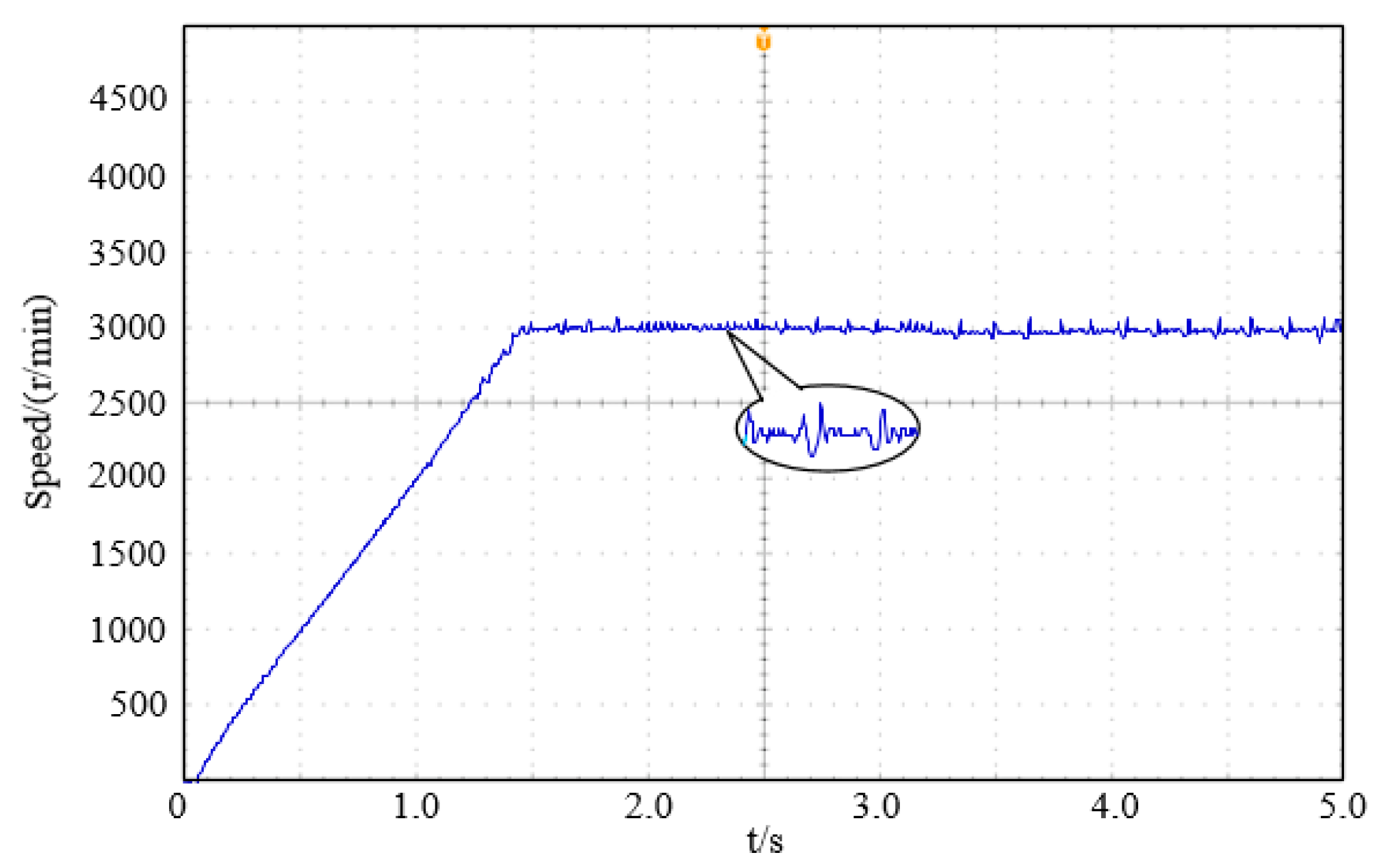
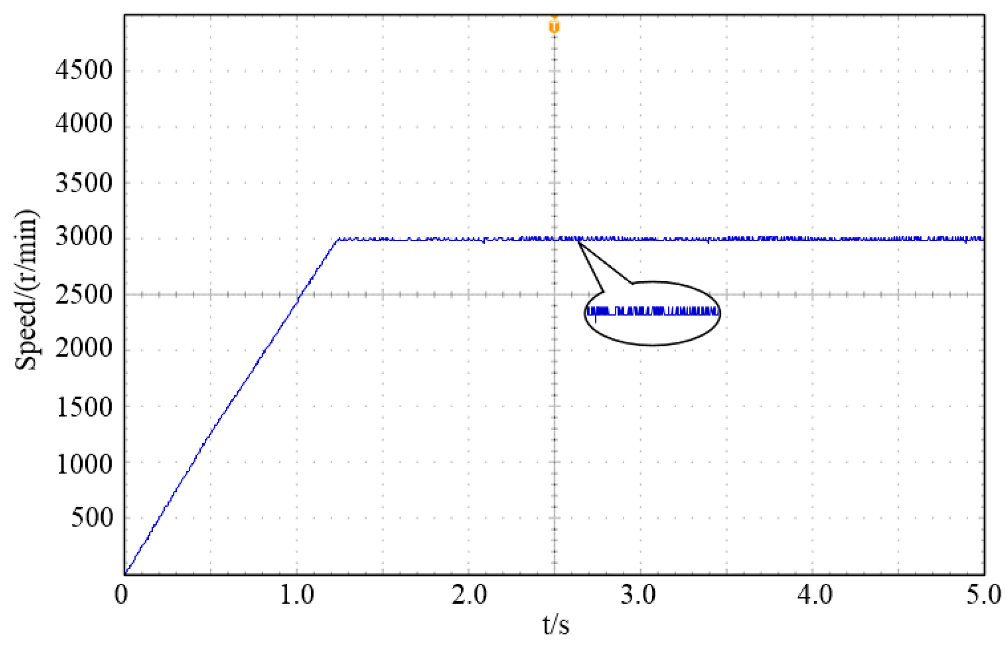
6. Development of the System Experiment Platform

The system experiment platform is mainly composed of a PMSM, motor controller, dynamometer and measurement and control system. The platform can complete the collection of vital information such as torque, rotation, voltage and current curve and power of the motor. Figure 8 is the experimental platform of the motor drive control system.

Set the motor speed to 3000 r/min, the load torque was 20 N·m in 0–10 s and increased to 70 N·m when t = 10 s. the current and speed response curves of the traditional and the improved field weakening control strategy are shown in Figure 9 and Figure 10. When compared, the improved field weakening control had a faster response and reduced system chattering.

When the load torque was 20 N·m and the motor increased from standstill to 3000 r/min, the speed response curves of the two strategies are shown in Figure 11 and Figure 12. When compared, the improved field weakening control strategy had a faster speed response and the jitter was substantially eliminated.

Figure 13 and Figure 14 show the current jitter curves for two control strategies. The traditional field weakening control strategy had obviously current jitter with a high risk of losing control. The jitter of this strategy was small and the stability of the system was high.

When the load torque was 70 N·m and the motor increased from standstill to 4000 r/min, the current dynamic response curves of the two control strategies are shown in Figure 15 and Figure 16. Before 1.0 s, the motor runs on the MTPA curve, i_d and i_q remained basically constant; 1.0–1.2s, the motor ran in the switching range between zone I and zone II; after 1.2 s, the motor ran in zone II, i_d and i_q weakened magnetic force at a constant value. The traditional flux weakening control strategy will have a sharp oscillation of d–q current during the weak magnetic acceleration phase. The improved field weakening control strategy can be smoothly switched between the MTPA zone and the field weakening control zone, ensuring a stable operation of the system at full speed and constant power output over a wide speed range.

Figure 17 shows the efficiency and speed curve for the rated conditions. In the field weakening control zone, this is when the speed exceeded 2000 r/min and the working efficiency of the motor was always above and below 96%, which fully met the efficiency requirements of the PMSM in the field weakening control zone.

7. Conclusions

This study proposed a field weakening control strategy based on feedback linearization. By using the principle of feedback linearization, the current controller selected a suitable feedback linear transformation and input transformation for a nonlinear PMSM system, so that the mathematical model of the system was linear relative to the new output. Decoupling control of d–q axis current was realized in a wide working area by using the flux linkage information of the motor without losing the controllability and accuracy of the system. In order to widen the motor speed regulation range and reduce the difficulty of algorithm implementation, the flux weakening control of PMSM was realized by using the current lead angle control method. Simulation and experimental results show that the system had strong robustness against load disturbances and obtains good steady characteristics and dynamic tracking performances.

References

1. Gu, W.; Zhu, X.; Quan, L.; Du, Y. Design and Optimization of Permanent Magnet Brushless Machines for Electric Vehicle Applications. Energies 2015, 8, 13996–14008. [Google Scholar] [CrossRef]
2. Liu, X.; Chen, H.; Zhao, J.; Belahcen, A. Research on the Performances and Parameters of Interior PMSM Used for Electric Vehicles. IEEE Trans. Ind. Electron. 2016, 63, 3533–3545. [Google Scholar] [CrossRef]
3. Fodorean, D.; Sarrazin, M.M.; Marţiş, C.S.; Anthonis, J.; Van der Auweraer, H. Electromagnetic and Structural Analysis for a Surface-Mounted PMSM Used for Light-EV. IEEE Trans. Ind. Appl. 2016, 52, 2892–2899. [Google Scholar] [CrossRef]
4. Shinohara, A.; Inoue, Y.; Morimoto, S.; Sanada, M. Maximum Torque Per Ampere Control in Stator Flux Linkage Synchronous Frame for DTC-Based PMSM Drives without Using q-Axis Inductance. IEEE Trans. Ind. Appl. 2017, 53, 3663–3671. [Google Scholar] [CrossRef]
5. Hoang, K.D.; Aorith, H.K.A. Online Control of IPMSM Drives for Traction Applications Considering Machine Parameter and Inverter Nonlinearities. IEEE Trans. Transp. Electrif. 2015, 1, 312–325. [Google Scholar] [CrossRef]
6. Zhang, Z.; Ge, X.; Tian, Z.; Zhang, X.; Tang, Q.; Feng, X. A PWM for Minimum Current Harmonic Distortion in Metro Traction PMSM with Saliency Ratio and Load Angle Constraints. IEEE Trans. Power Electron. 2017, 33, 4498–4511. [Google Scholar] [CrossRef]
7. Liang, W.; Wang, J.; Luk, P.C.; Fang, W.; Fei, W. Analytical Modeling of Current Harmonic Components in PMSM Drive with Voltage-Source Inverter by SVPWM Technique. IEEE Trans. Energy Convers. 2014, 29, 673–680. [Google Scholar] [CrossRef]
8. Yamamoto, K.; Shinohara, K.; Nagahama, T. Characteristics of permanent-magnet synchronous motor driven by PWM inverter with voltage booster. IEEE Trans. Ind. Appl. 2004, 40, 1145–1152. [Google Scholar] [CrossRef]
9. Zhong, Q.C.; Rees, D. Control of uncertain LTI systems based on an uncertainty and disturbance estimator. ASME J. Dyn. Syst. Meas. Control 2004, 126, 905–910. [Google Scholar] [CrossRef]
10. Gu, X.; Li, T.; Li, X.; Zhang, G.; Wang, Z. An Improved UDE-Based Flux-Weakening Control Strategy for IPMSM. Energies 2019, 12, 4077. [Google Scholar] [CrossRef]
11. Lin, F.J.; Sun, I.F.; Yang, K.J.; Chang, J.K. Recurrent Fuzzy Neural Cerebellar Model Articulation Network Fault-Tolerant Control of Six-Phase Permanent Magnet Synchronous Motor Position Servo Drive. IEEE Trans. Fuzzy Syst. 2016, 24, 153–167. [Google Scholar] [CrossRef]
12. Yu, J.; Chen, B.; Yu, H.; Lin, C.; Ji, Z.; Cheng, X. Position tracking control for chaotic permanent magnet synchronous motors via indirect adaptive neural approximation. Neurocomputing 2015, 156, 245–251. [Google Scholar] [CrossRef]
13. Wang, T.; Huang, J.; Ye, M.; Chen, J.; Kong, W.; Kang, M.; Yu, M. An EMF Observer for PMSM Sensorless Drives Adaptive to Stator Resistance and Rotor Flux-linkage. IEEE J. Emerg. Sel. Top. Power Electron 2019, in press. [Google Scholar] [CrossRef]
14. Zhou, K.; Ai, M.; Sun, Y.; Wu, X.; Li, R. PMSM Vector Control Strategy Based on Active Disturbance Rejection Controller. Energies 2019, 12, 3827. [Google Scholar] [CrossRef]
15. Andersson, A.; Thiringer, T. Assessment of an Improved Finite Control Set Model Predictive Current Controller for Automotive Propulsion Applications. IEEE Trans. Ind. Electron. 2019, 67, 91–100. [Google Scholar] [CrossRef]
16. Cortes, P.; Kazmierkowski, M.P.; Kennel, R.M.; Quevedo, D.E.; Rodriguez, J. Predictive Control in Power Electronics and Drives. IEEE Trans. Ind. Electron. 2008, 55, 4312–4324. [Google Scholar] [CrossRef]
17. Chai, S.; Wang, L.; Rogers, E. A Cascade MPC Control Structure for a PMSM with Speed Ripple Minimization. IEEE Trans. Ind. Electron. 2013, 60, 2978–2987. [Google Scholar] [CrossRef]
18. Lin, C.K.; Yu, J.T.; Lai, Y.S.; Yu, H.C. Improved Model-Free Predictive Current Control for Synchronous Reluctance Motor Drives. IEEE Trans. Ind. Electron. 2016, 63, 3942–3953. [Google Scholar] [CrossRef]
19. Inoue, Y.; Morimoto, S.; Sanada, M. Comparative Study of PMSM Drive Systems Based on Current Control and Direct Torque Control in Flux-Weakening Control Region. IEEE Trans. Ind. Appl. 2012, 48, 2382–2389. [Google Scholar] [CrossRef]
20. Foo, G.H.B.; Zhang, X. Robust Direct Torque Control of Synchronous Reluctance Motor Drives in the Field-Weakening Region. IEEE Trans. Power Electron. 2017, 32, 1289–1298. [Google Scholar] [CrossRef]
21. Pellegrino, G.; Bojoi, R.I.; Guglielmi, P. Unified Direct-Flux Vector Control for AC Motor Drives. IEEE Trans. Ind. Appl. 2011, 47, 2093–2102. [Google Scholar] [CrossRef]
22. Yousefi-Talouki, A.; Pescetto, P.; Pellegrino, G. Sensorless Direct Flux Vector Control of Synchronous Reluctance Motors Including Standstill, MTPA, and Flux Weakening. IEEE Trans. Ind. Appl. 2017, 53, 3598–3608. [Google Scholar] [CrossRef]
23. Liu, H.; Zhu, Z.; Mohamed, E.; Fu, Y.; Qi, X. Flux-Weakening Control of Nonsalient Pole PMSM Having Large Winding Inductance, Accounting for Resistive Voltage Drop and Inverter Nonlinearities. IEEE Trans. Power Electron. 2012, 27, 942–952. [Google Scholar] [CrossRef]
24. Jung, S.Y.; Mi, C.C.; Nam, K. Torque Control of IPMSM in the Field-Weakening Region with Improved DC-Link Voltage Utilization. IEEE Trans. Ind. Electron. 2015, 62, 3380–3387. [Google Scholar] [CrossRef]
25. Zhang, X.; Zhang, L.; Zhang, Y. Model Predictive Current Control for PMSM Drives with Parameter Robustness Improvement. IEEE Trans. Power Electron. 2019, 34, 1645–1657. [Google Scholar] [CrossRef]
26. Mohseni, M.; Islam, S.M.; Masoum, M.A.S. Impacts of symmetrical and asymmetrical voltage sags ondfig-based wind turbines considering phase-angle jump, voltage recovery, and sag parameters. IEEE Trans. Power Electron. 2011, 26, 1587–1598. [Google Scholar] [CrossRef]
27. Wang, W.; Zhang, J.; Cheng, M. Line-modulation-based flux-weakening control for permanent-magnet synchronous machines. IET Power Electron. 2018, 11, 930–936. [Google Scholar] [CrossRef]
28. Lai, G.; Liu, Z.; Zhang, Y.; Chen, C.L.P.; Xie, S.; Liu, Y. Fuzzy Adaptive Inverse Compensation Method to Tracking Control of Uncertain Nonlinear Systems with Generalized Actuator Dead Zone. IEEE Trans. Fuzzy Syst. 2017, 25, 191–204. [Google Scholar] [CrossRef]
29. Inoue, T.; Inoue, Y.; Morimoto, S.; Sanada, M. Maximum Torque per Ampere Control of a Direct Torque-Controlled PMSM in a Stator Flux Linkage Synchronous Frame. IEEE Trans. Ind. Appl. 2016, 52, 2630–2637. [Google Scholar] [CrossRef]
30. Mynar, Z.; Vesely, L.; Vaclavek, P. PMSM Model Predictive Control with Field-Weakening Implementation. IEEE Trans. Ind. Electron. 2016, 63, 5156–5166. [Google Scholar] [CrossRef]
31. Jo, C.; Seol, J.Y.; Ha, I.J. Flux-Weakening Control of IPM Motors with Signifificant Effffect of Magnetic Saturation and Stator Resistance. IEEE Trans. Ind. Electron. 2008, 55, 1330–1340. [Google Scholar]
32. Schoonhoven, G.; Uddin, M.N. MTPA- and FW-Based Robust Nonlinear Speed Control of IPMSM Drive Using Lyapunov Stability Criterion. IEEE Trans. Ind. Appl. 2016, 52, 4365–4374. [Google Scholar] [CrossRef]
33. Dong, Z.; Yu, Y.; Li, W.; Wang, B.; Xu, D. Flux-Weakening Control for Induction Motor in Voltage Extension Region: Torque Analysis and Dynamic Performance Improvement. IEEE Trans. Ind. Electron. 2018, 65, 3740–3751. [Google Scholar] [CrossRef]
34. Ren, B.; Zhong, Q.C.; Chen, J. Robust Control for a Class of Nonaffine Nonlinear Systems Based on the Uncertainty and Disturbance Estimator. IEEE Trans. Ind. Electron. 2015, 62, 5881–5888. [Google Scholar] [CrossRef]
35. Zhang, Z.; Wang, C.; Zhou, M.; You, X. Flux-Weakening in PMSM Drives: Analysis of Voltage Angle Control and the Single Current Controller Design. IEEE J. Emerg. Sel. Top. Power Electron. 2019, 7, 437–445. [Google Scholar] [CrossRef]
Figure 1. Variation of flux magnitude on the constant torque curves.
Energies 12 04526 g001
Figure 2. Operating point trajectory of flux weakening (FW).
Energies 12 04526 g002
Figure 3. Space vector permanent magnet synchronous motor (PMSM) diagram.
Energies 12 04526 g003
Figure 4. Improved FW operation control strategy.
Energies 12 04526 g004
Figure 5. Speed response curve.
Energies 12 04526 g005
Figure 6. The current response curve of the d-axis.
Energies 12 04526 g006
Figure 7. The current response curve of the q-axis.
Energies 12 04526 g007
Figure 8. Test platform.
Energies 12 04526 g008
Figure 9. Speed response curve.
Energies 12 04526 g009
Figure 10. Current response curve of the d–q axis.
Energies 12 04526 g010
Figure 11. Traditional FW speed response curve.
Energies 12 04526 g011
Figure 12. Improved FW speed response curve.
Energies 12 04526 g012
Figure 13. Traditional FW algorithm current jitter curve.
Energies 12 04526 g013
Figure 14. Improved FW current jitter curve.
Energies 12 04526 g014
Figure 15. The current dynamic response curve of traditional FW at the d–q axis.
Energies 12 04526 g015
Figure 16. The current response curve of improved FW at the d–q axis.
Energies 12 04526 g016
Figure 17. Efficiency/speed characteristic curve.
Energies 12 04526 g017