Source Term Modelling of Vane-Type Vortex Generators under Adverse Pressure Gradient in OpenFOAM


Abstract
1. Introduction
2. Theoretical Background
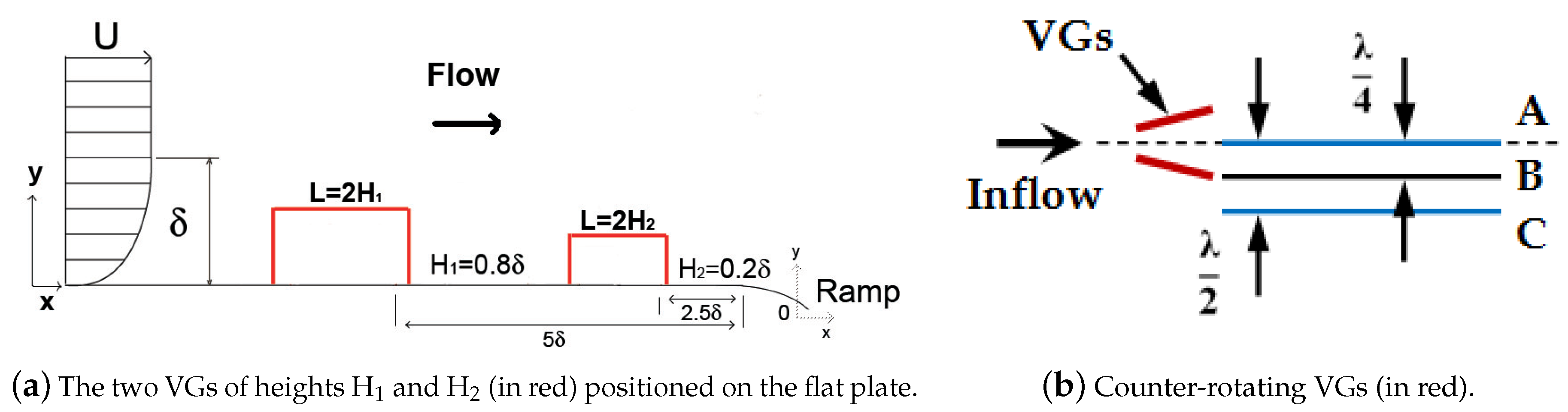
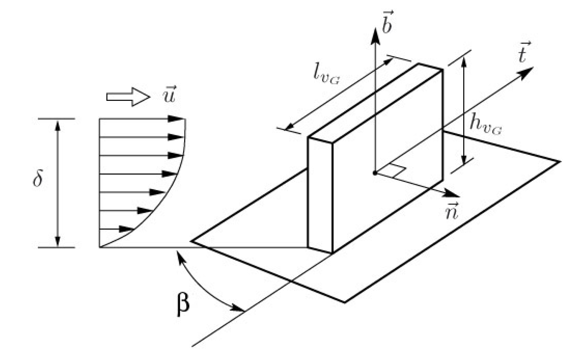
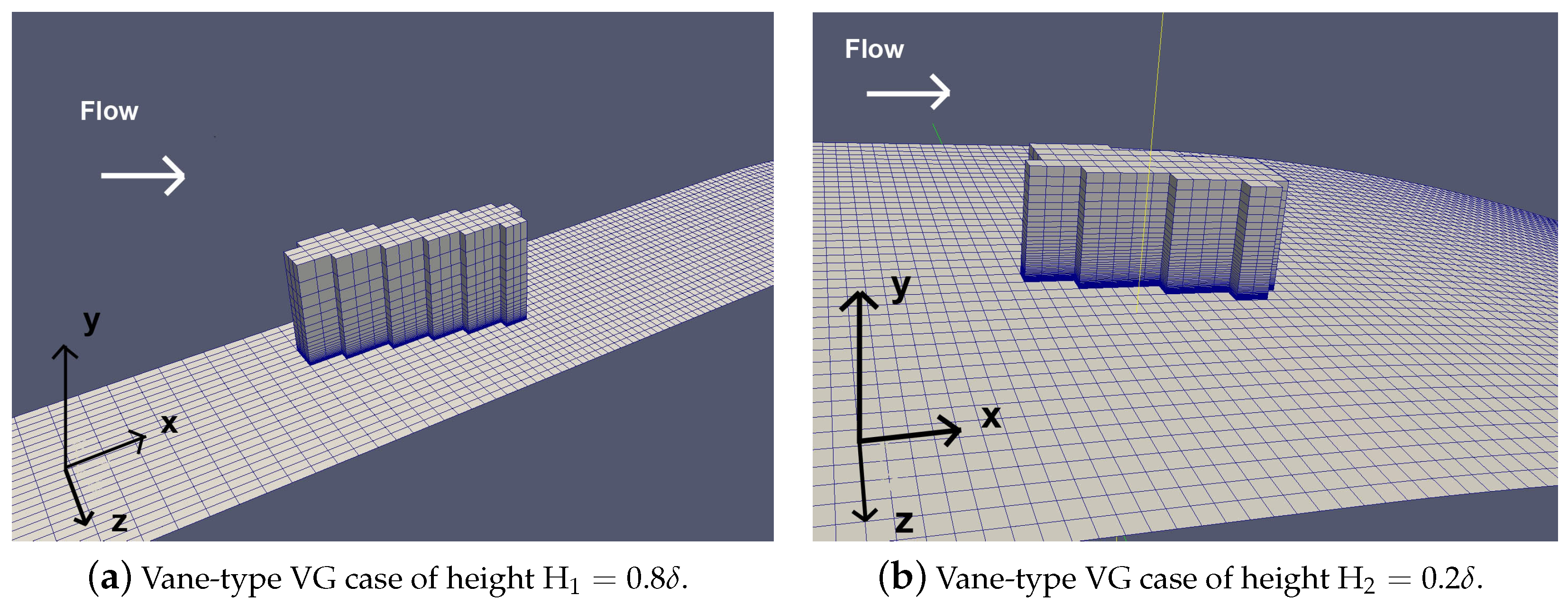
2.1. Vortex Generator Setup
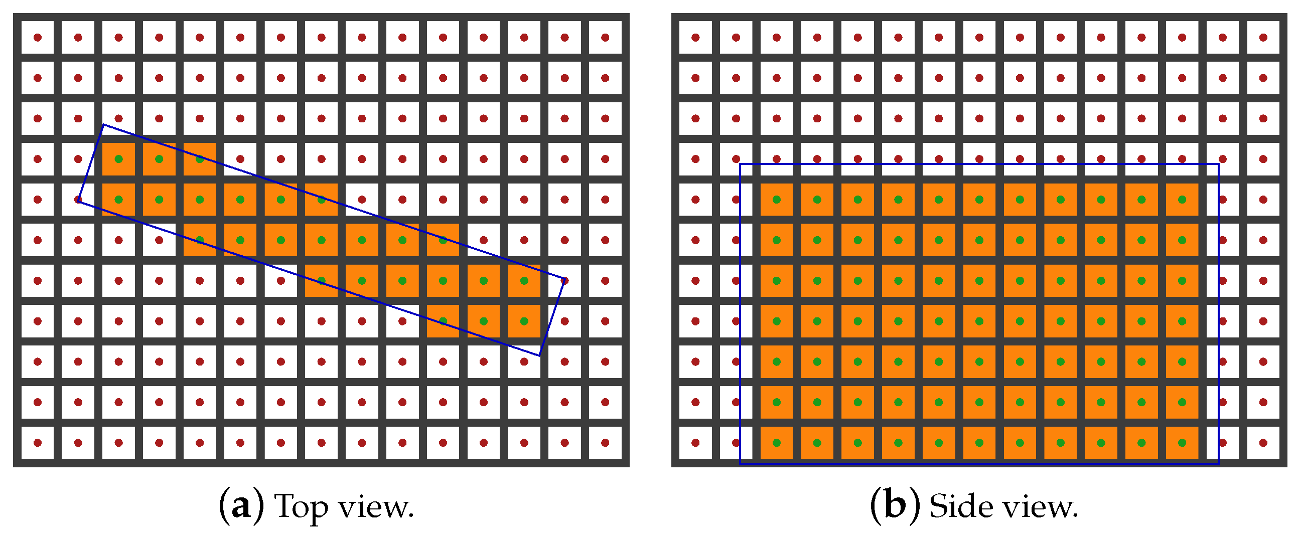
2.2. Source Term Model
3. Experimental Data
4. Computational Configuration
5. Results
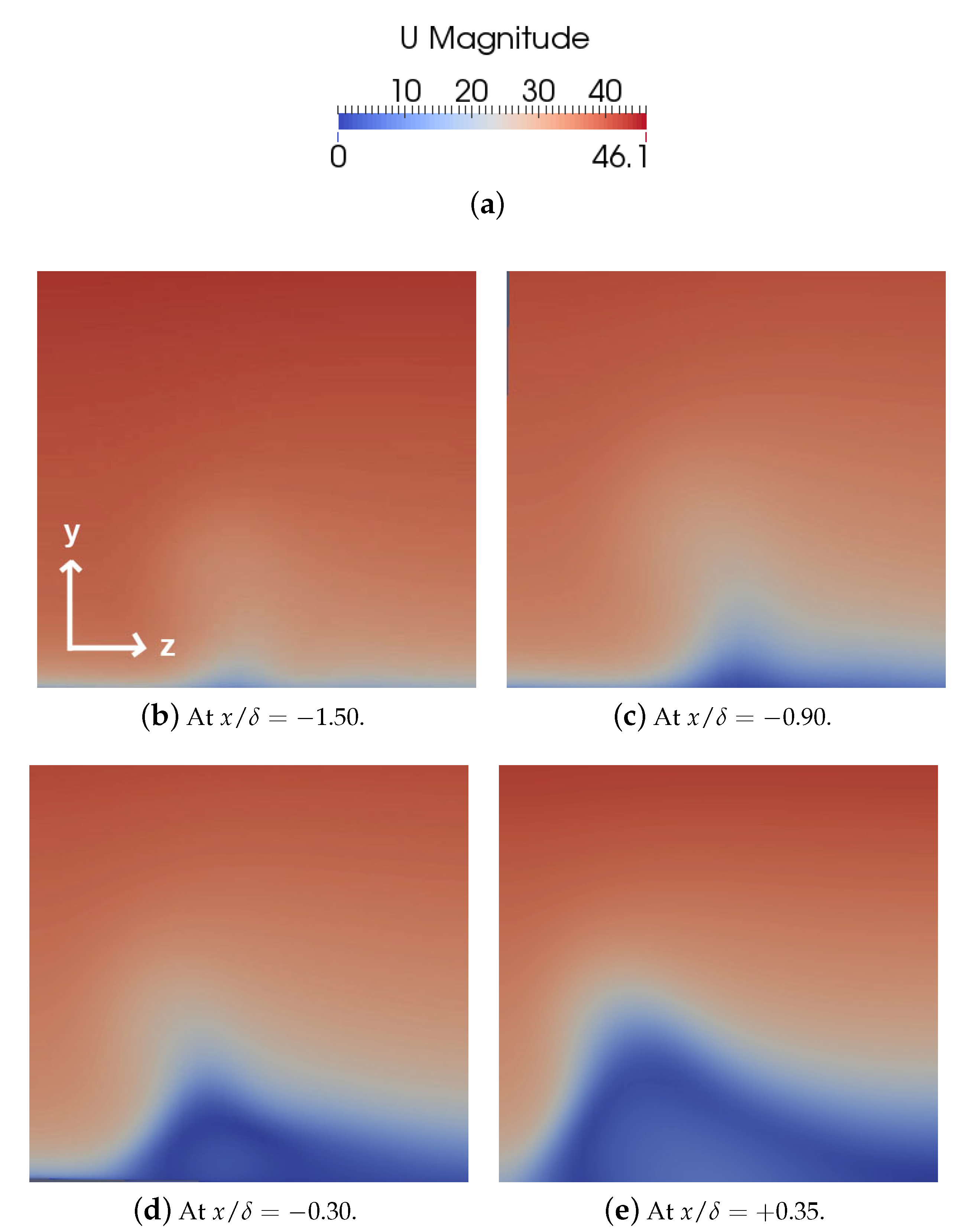
5.1. Vortex Visualization
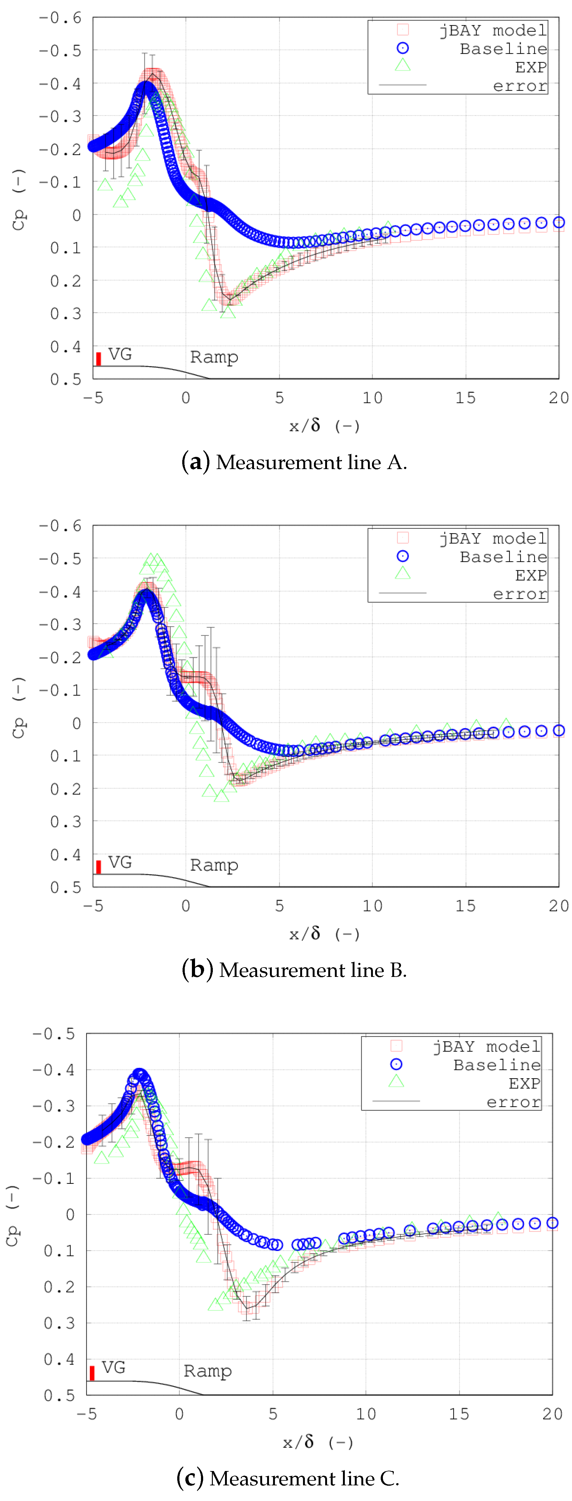
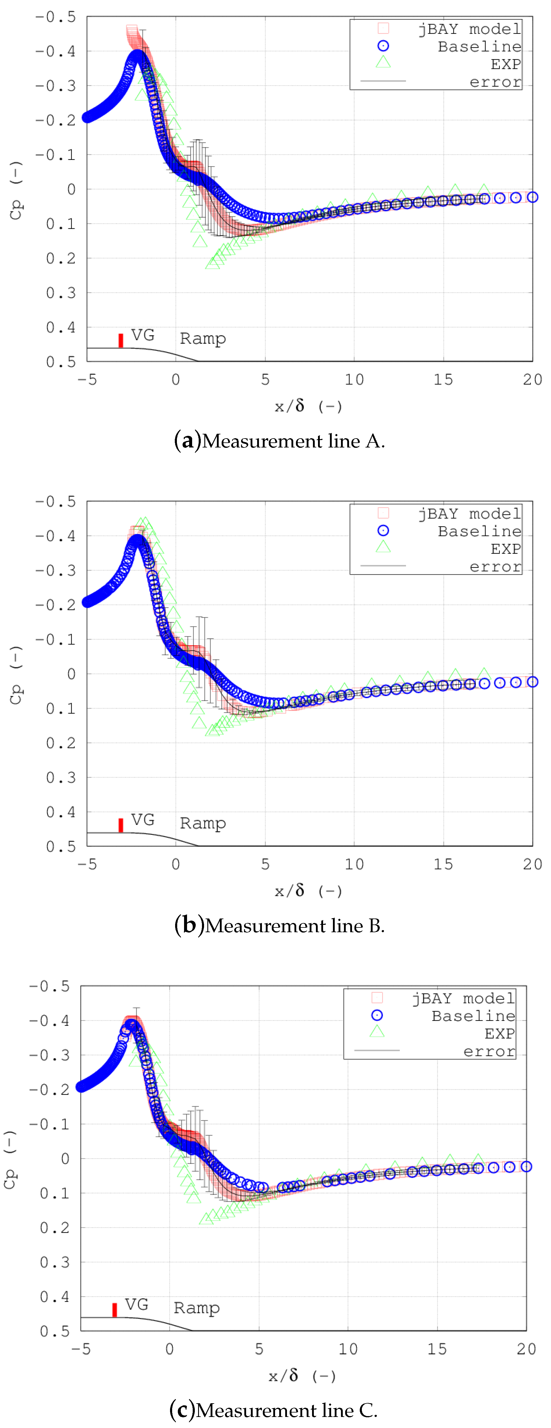
5.2. Pressure Distribution
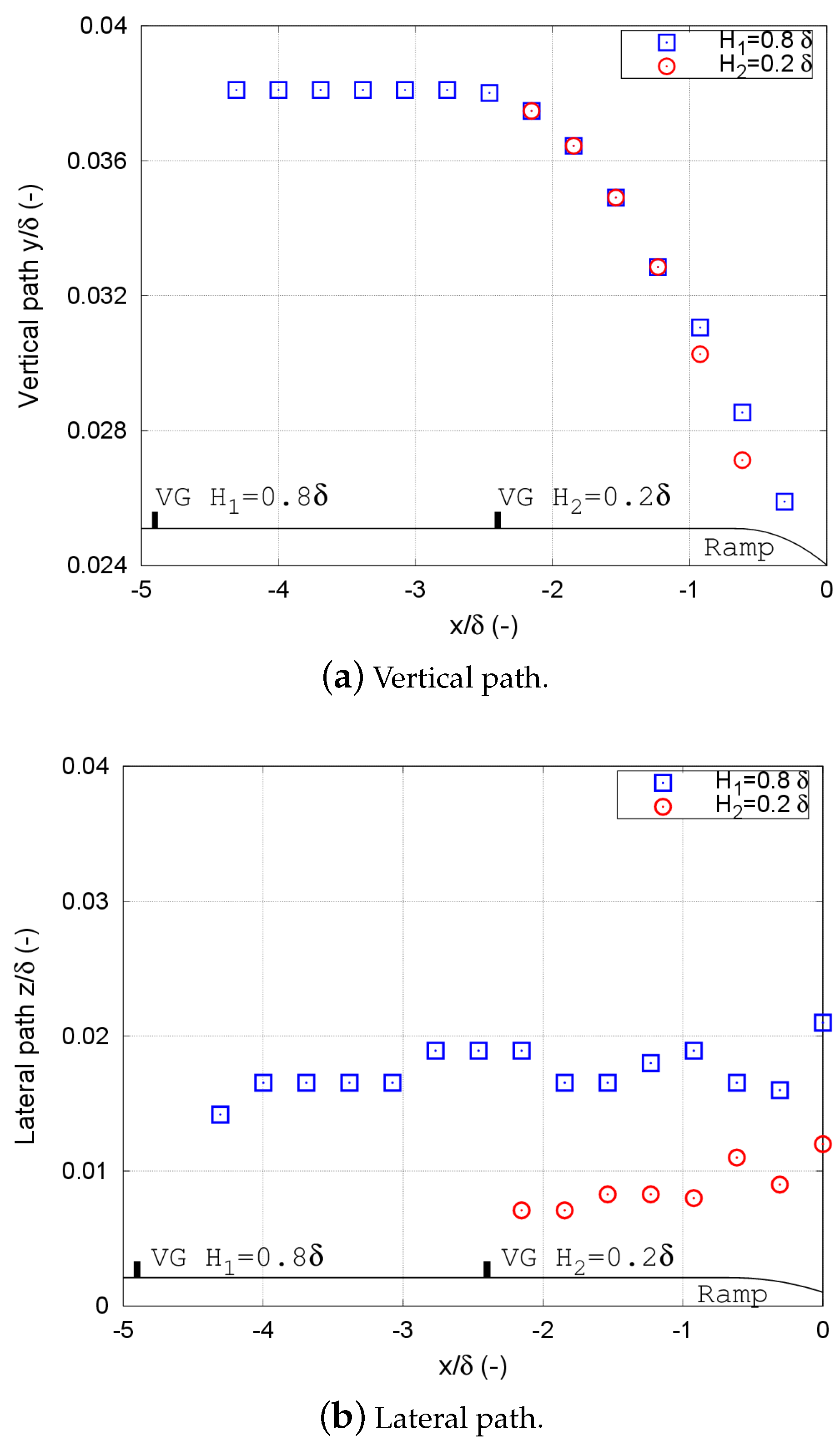
5.3. Vortex Path
5.4. Vortex Decay
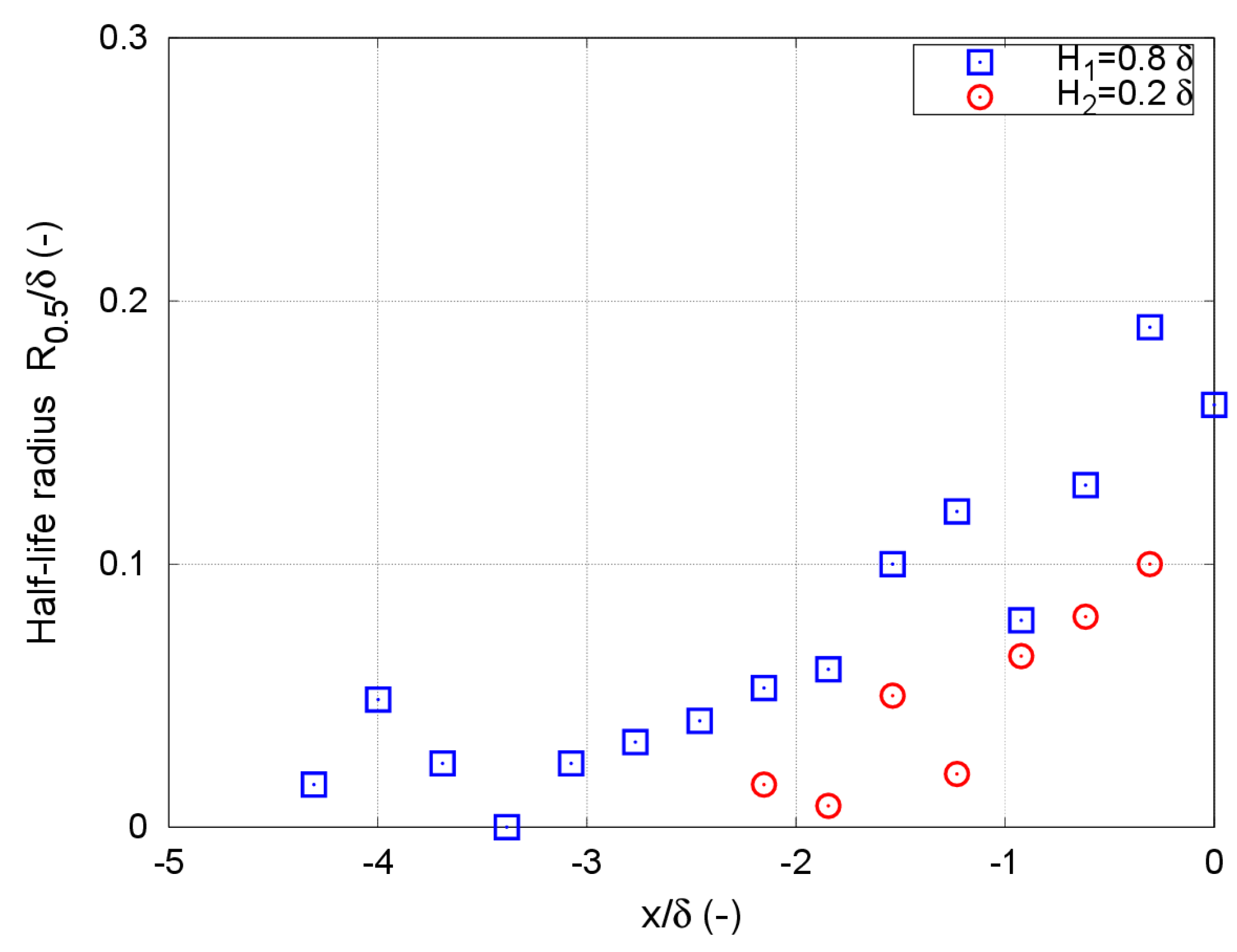
5.5. Vortex Size
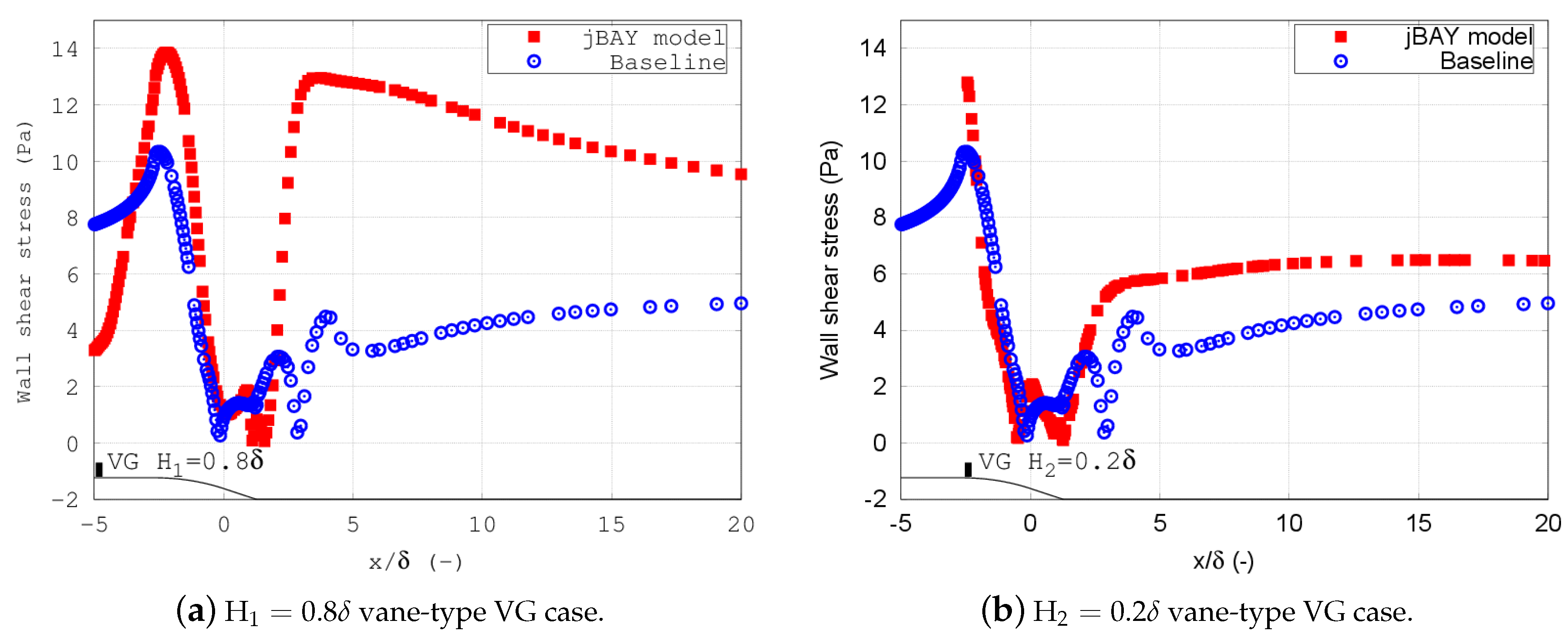
5.6. Wall Shear Stress
6. Conclusions
Author Contributions
Funding
Acknowledgments
Conflicts of Interest
References
- Johnson, S.J.; Baker, J.P.; van Dam, C.P.; Berg, D. An overview of active load control techniques for wind turbines with an emphasis on microtabs. Wind Energy 2009, 13, 239–253. [Google Scholar] [CrossRef]
- Gad-el-Hak, M. Flow Control: Passive, Active, and Reactive Flow Management; Cambridge University Press: Cambridge, UK, 2007; ISBN 9780521036719. [Google Scholar]
- Taylor, H.D. Summary Report on Vortex Generators; Research Department Report No. R-05280-9; Research Department, United Aircraft Corporation: Moscow, Russia, 1947. [Google Scholar]
- Liu, Y.; Sun, J.; Tang, Y.; Lu, L. Effect of slot at blade root on compressor cascade performance under different aerodynamic parameters. Appl. Sci. 2016, 6, 421. [Google Scholar] [CrossRef]
- Wood, R.M. Discussion of aerodynamic control effectors concepts (ACEs) for future unmanned air vehicles (UAVs). In Proceedings of the AIAA 1st Technical Conference and Workshop on Unmanned Aerospace Vehicle, Systems, Technologies and Operations, Portsmouth, VA, USA, 20–23 May 2002. [Google Scholar]
- Aramendia, I.; Fernández-Gamiz, U.; Ramos-Hernanz, J.A.; Sancho, J.; Lopez-Guede, J.M.; Zulueta, E. Flow Control Devices for Wind Turbines. Energy Harvest. Energy Effic. Technol. Methods Appl. 2017, 37, 629–655. [Google Scholar] [CrossRef]
- Becker, R.; Garwon, M.; Gutknecht, C.; Barwolff, G.; King, R. Robust control of separated shear flows in simulation and experiment. J. Process Control 2005, 15, 691–700. [Google Scholar] [CrossRef]
- Rao, D.M.; Kariya, T.T. Boundary-layer submerged vortex generators for separation control, an exploratory study. In Proceedings of the AIAA/ASME/SIAM/APS 1st National Fluid Dynamics Congress, Cincinnati, OH, USA, 25–28 July1998. [Google Scholar]
- Lin, J.C.; Robinson, S.K.; McGhee, R.J.; Valarezo, W.O. Separation Control on high-lift airfoils via micro vortex generators. J. Aircr. 1994, 31, 1317–1323. [Google Scholar] [CrossRef]
- Doerffer, P.; Barakos, G.N.; Luczak, M.M. Recent Progress in Flow Control for Practical Flows. In Results of the STADYWICO and IMESCON Projects; Springer International Publishing AG: Cham, Switzerland, 2017; ISBN 978-3-319-50568-8. [Google Scholar]
- Steijl, R.; Barakos, G.; Badcock, K. A framework for CFD analysis of helicopter rotors in hover and forward flight. Int. J. Numer. Methods Fluids 2006, 51, 819–847. [Google Scholar] [CrossRef]
- Velte, C.M.; Hansen, M.O.L. Investigation of flow behind vortex generators by stereo particle image velocimetry on a thick airfoil near stall. Wind Energy 2013, 16, 775–785. [Google Scholar] [CrossRef]
- Velte, C.M.; Hansen, M.O.L.; Okulov, V.L. Helical structure of longitudinal vortices embedded in turbulent wall-bounded flow. J. Fluid Mech. 2009, 619, 167–177. [Google Scholar] [CrossRef]
- Fernández-Gamiz, U.; Velte, C.M.; Réthoré, P.; Sørensen, N.N.; Egusquiza, E. Testing of self-similarity and helical symmetry in vortex generator flow simulations. Wind Energy 2016, 19, 1043–1052. [Google Scholar] [CrossRef]
- Urkiola, A.; Fernández-Gamiz, U.; Errasti, I.; Zulueta, E. Computational characterization of the vortex generated by a vortex generator on a flat plate for different vane angles. Aerosp. Sci. Technol. 2017, 65, 18–25. [Google Scholar] [CrossRef]
- Gao, L.; Zhang, H.; Liu, Y.; Han, S. Effects of vortex generators on a blunt trailing-edge airfoil for wind turbines. Renew. Energy 2015, 76, 303–311. [Google Scholar] [CrossRef]
- Baldacchino, D.; Manolesos, M.; Ferreira, C.; Gonzalez Salcedo, A.; Aparicio, M.; Chaviaropoulos, T.; Diakakis, K.; Florentie, L.; Garcia, N.R.; Papadakis, G.; et al. Experimental benchmark and code validation for airfoils equipped with passive vortex generators. J. Phys. 2016, 753, 022002. [Google Scholar] [CrossRef]
- Keuthe, A.M. Effect of streamwise vortices on wake properties associated with sound generation. J. Aircr. 1972, 9, 715–719. [Google Scholar] [CrossRef]
- Holmes, A.; Hickey, P.; Murphy, W.; Hilton, D. The application of sub-boundary layer vortex generators to reduce canopy “Mach rumble” interior noise on the Gulfstream III. In Proceedings of the 25th AIAA Aerospace Sciences Meeting, Aerospace Sciences Meetings, Reno, NV, USA, 24–26 March 1987. [Google Scholar] [CrossRef]
- Lin, J.C.; Howard, F.G.; Selby, G.V. Small submerged vortex generators for turbulent-flow separation control. J. Spacecr. Rocket. 1990, 27, 503–507. [Google Scholar] [CrossRef]
- Martinez-Filgueira, P.; Fernández-Gamiz, U.; Zulueta, E.; Errasti, I.; Fernández-Gauna, B. Parametric study of low-profile vortex generators. Int. J. Hydrogen Energy 2017, 42, 17700–17712. [Google Scholar] [CrossRef]
- Lin, J. Review of research on low-profile vortex generators to control boundary-layer separation. Prog. Aerosp. Sci. 2002, 38, 389–420. [Google Scholar] [CrossRef]
- Kenning, O.C.; Kaynes, I.W.; Miller, J.V. The potential application of flow control to helicopter rotor blades. In Proceedings of the 30th European Rotorcraft Forum, Marseille, France, 14–16 September 2004; 14p. [Google Scholar]
- Schubauer, G.B.; Spangenber, W.G. Forced mixing in boundary layers. J. Fluid Mech. 1960, 8, 10–32. [Google Scholar] [CrossRef]
- Bragg, M.B.; Gregorek, G.M. Experimental study of airfoil performance with vortex generators. J. Aircr. 1987, 24, 305–309. [Google Scholar] [CrossRef]
- Fernández-Gamiz, U.; Errasti, I.; Gutierrez-Amo, R.; Boyano, A.; Barambones, O. Computational modelling of rectangular sub-boundary-layer vortex generators. Appl. Sci. 2018, 8, 138. [Google Scholar] [CrossRef]
- Troldborg, N.; Zahle, F.; Sorensen, N.N. Simulation of a MW rotor equipped with vortex generators using CFD and an actuator shape model. In Proceedings of the 53th AIAA Aerospace Sciences Meeting, Kissimmee, FL, USA, 5–9 January 2015; 10p. [Google Scholar]
- Bender, E.E.; Anderson, B.H.; Yagle, P.J. Vortex Generator Modelling for Navier–Stokes Codes. In Proceedings of the 3rd ASME/JSME Joint Fluids Engineering Conference, San Francisco, CA, USA, 18–23 July 1999. [Google Scholar]
- Dudek, J.C. Modeling Vortex Generators in a Navier–Stokes Code. AIAA J. 2011, 49, 748–759. [Google Scholar] [CrossRef]
- Jirasek, A. Vortex-Generator Model and Its Application to Flow Control. J. Aircr. 2005, 42, 1486–1491. [Google Scholar] [CrossRef]
- Florentie, L.; Hulshoff, S.J.; van Zuijlen, A.H. Adjoint-based optimization of a source-term representation of vortex generators. Comput. Fluids 2018, 162, 139–151. [Google Scholar] [CrossRef]
- OpenFOAM. Available online: https://openfoam.org (accessed on 1 October 2018).
- Lin, J.C. Control of Turbulent Boundary-Layer Separation using Micro-Vortex Generators. Am. Inst. Aeronaut. Astronaut. 1999, 1–16. [Google Scholar] [CrossRef]
- Konig, B.; Fares, E.; Nolting, S. Fully-Resolved Lattice-Boltzmann Simulation of Vane-Type Vortex Generators. In Proceedings of the 7th AIAA Flow Control Conference, Atlanta, GA, USA, 16–20 June 2014; pp. 2795–3008. [Google Scholar] [CrossRef]
- Menter, F.R. Zonal two equation k-w turbulence model for aerodynamic flows. AIAA J. 1993, 93, 2906. [Google Scholar] [CrossRef]
- Gutierrez-Amo, R.; Fernández-Gamiz, U.; Errasti, I.; Zulueta, E. Computational modelling of three different sub-boundary layer vortex generators on a flat plate. Energies 2018, 11, 3107. [Google Scholar] [CrossRef]
- Sørensen, N.; Zahle, F.; Bak, C.; Vronsky, T. Prediction of the Effect of Vortex Generators on Airfoil Performance. Phys. Conf. Ser. 2014, 524, 012019. [Google Scholar] [CrossRef]
- Richardson, L.F.; Gaunt, J.A. The deferred approach to the limit. Part I. Single lattice. Part II. Interpenetrating lattices. Philos. Trans. R. Soc. Lond. Ser. A 1927, 226, 299–361. [Google Scholar] [CrossRef]
- Fernández-Gamiz, U.; Zamorano, G.; Zulueta, E. Computational study of the vortex path variation with the VG height. J. Phys. Conf. Ser. 2014, 524, 012024. [Google Scholar] [CrossRef]
- Bray, T.P. A Parametric Study of Vane and Air-Jet Vortex Generators. Ph.D. Thesis, College of Aeronautics, Cranfield University, Cranfield, UK, 1998. [Google Scholar]
- Godard, G.; Stanislas, M. Control of a decelerating boundary layer. Part 1. Optimization of passive vortex generators. Aerosp. Sci. Technol. 2006, 10, 181–191. [Google Scholar] [CrossRef]


| VG Parameter | H VG Case | H VG Case |
|---|---|---|
| Height H | 0.8 | 0.2 |
| Length L | 1.6 | 0.4 |
| Incident angle | 15 | 25 |
| Location from the ramp | 5 | 2.5 |
| Spacing | 3.2 | 0.8 |
| VG Case | Non-Orthogonality (Average) | Maximum Skewness (-) | |
|---|---|---|---|
| H | 5.44 | 0.56 | |
| H | 5.32 | 0.38 |
| VG Case | Plane Location | Peak Coarse | Vorticity Medium | ()/ (-) Fine | RE | p | R |
|---|---|---|---|---|---|---|---|
| H | 74.25 | 122.78 | 128.32 | 127.61 | 3.13 | 0.11 | |
| H | 12.00 | 27.91 | 29.54 | 29.35 | 3.29 | 0.10 |
| VG Case | Minimum | Maximum | Average |
|---|---|---|---|
| H | 0.14 | 1.29 | 0.64 |
| H | 0.06 | 0.71 | 0.35 |
© 2019 by the authors. Licensee MDPI, Basel, Switzerland. This article is an open access article distributed under the terms and conditions of the Creative Commons Attribution (CC BY) license (http://creativecommons.org/licenses/by/4.0/).
Share and Cite
Errasti, I.; Fernández-Gamiz, U.; Martínez-Filgueira, P.; Blanco, J.M. Source Term Modelling of Vane-Type Vortex Generators under Adverse Pressure Gradient in OpenFOAM. Energies 2019, 12, 605. https://doi.org/10.3390/en12040605
Errasti I, Fernández-Gamiz U, Martínez-Filgueira P, Blanco JM. Source Term Modelling of Vane-Type Vortex Generators under Adverse Pressure Gradient in OpenFOAM. Energies. 2019; 12(4):605. https://doi.org/10.3390/en12040605
Chicago/Turabian StyleErrasti, Iñigo, Unai Fernández-Gamiz, Pablo Martínez-Filgueira, and Jesús María Blanco. 2019. "Source Term Modelling of Vane-Type Vortex Generators under Adverse Pressure Gradient in OpenFOAM" Energies 12, no. 4: 605. https://doi.org/10.3390/en12040605
APA StyleErrasti, I., Fernández-Gamiz, U., Martínez-Filgueira, P., & Blanco, J. M. (2019). Source Term Modelling of Vane-Type Vortex Generators under Adverse Pressure Gradient in OpenFOAM. Energies, 12(4), 605. https://doi.org/10.3390/en12040605